Linear and Nonlinear Experimental Regimes of Stochastic Resonance

Abstract

We investigate the stochastic resonance phenomenon in a physical system based on a tunnel diode. The experimental control parameters are set to allow the control of the frequency and amplitude of the deterministic modulating signal over an interval of values spanning several orders of magnitude. We observe both a regime described by the linear response theory and the nonlinear deviation from it. In the nonlinear regime we detect saturation of the power spectral density of the output signal detected at the frequency of the modulating signal and a dip in the noise level of the same spectral density. When these effects are observed we detect a phase and frequency synchronization between the stochastic output and the deterministic input.

05.40.-a, 85.30.Mn

]

I Introduction.

The renewed interest of the last two decades on stochastic processes modeling different phenomena of physics, chemistry and engineering sciences has led to the discovery of noise-induced phenomena in nonlinear systems away from equilibrium. In these systems a variation of the level of external noise can qualitatively change the response of the system. The paradigmatic example of these noise-induced phenomena is stochastic resonance [1] (for a recent review see [2]). Other examples of noise-induced phenomena comprise resonant activation [3], noise-induced transitions [4] and noise enhanced stability [5, 6].

Stochastic resonance (SR) manifests itself as an enhancement of the system response for certain finite values of the noise strength. In particular the signal-to-noise ratio (SNR) shows a maximum as a function of the noise intensity. In other words, a statistical synchronization of the random transitions between the two metastable states of the nonlinear system takes place in the presence of an external weak periodic force and noise. Such a physical system presents a time-scale matching condition, which can be observed by tuning the noise level to such a value that the period of the driving force approximately equals twice the noise-induced escape time. The SR phenomenon appears in a large variety of physical systems and has been observed in different systems, ranging from sets of neurons [7], to lasers [8] and to solid-state devices, like SQUIDs and tunnel diodes [9].

The SR phenomenon is a well investigated phenomenon both from a theoretical and an experimental point of view [2]. However, few studies systematically analyze the SR phenomenon for different values of the frequency and amplitude of the modulating signal [8, 9, 10, 11, 12]. In this article we systematically study the SR phenomenon as a function of the frequency and amplitude of the modulating signal in a physical bistable system based on a tunnel diode. Our experimental set-up allows us to investigate this phenomenon in a range of amplitude and frequency spanning several orders of magnitude. By varying the amplitude and the frequency of the modulating signal we detect both the regime of the SR phenomenon described by the linear response theory and the nonlinear deviation from it. In the linear regime we observe the customary behavior of stochastic resonance whereas in the nonlinear regime we detect a saturation of the power spectral density measured at the frequency of the modulating signal and a depletion of the power spectral density of the noise at the same frequency. When the noise depletion takes place we observe phase and frequency synchronization between the stochastic output and the deterministic input.

The paper is organized as follows. In section II we describe the experimental apparatus and we discuss the stochastic differential equation associated to the electronic circuit based on a tunnel diode. In section III we present our experimental results of the power amplification and SNR as a function of the noise intensity for different values of the amplitude and frequency of the modulating signal. In this section we discuss the detected deviations form the predictions of the linear response theory and we present an evidence of phase and frequency synchronization detected in the nonlinear regime of high values of the amplitude of the modulating signal. In section IV we briefly draw our conclusions.

II Experimental apparatus and the tunnel diode

The experimental setup used for investigating the SR phenomenon is a bistable electronic system based on a tunnel diode. The physical system is a series of a resistor(tunable to a desired value) and a tunnel diode in parallel to a capacitor. The tunnel diode is a highly doped semiconductor device with a typical current-voltage characteristic showing a region of negative differential resistance, which is due to a tunneling current from the valence band of the n-doped region to the conducting band of the p-doped region. There are two stable states and one unstable state [13, 14, 15]. For details about this experimental set-up see ref. [16].

A network of general purpose very low-noise wide band operational amplifier is used to sum the driving periodic signal and the noise signal. The noise signal is the output of a commercial digital noise source, whose spectral density is approximately flat up to 20 MHz and whose root mean square voltage $V_{rms}$ may be selected within the range from $0.133$ to $5.5$ V with a 27 mV resolution. At the output of the operational amplifier the statistical properties of the noise are altered by the filtering of the operational amplifier. We measure the noise $v_{n}(t)$ at the output of the operational amplifier and we observe that it is a Gaussian noise characterized by a spectral density which is flat at low frequency ($f<1.25$ MHz). By defining the correlation time of the Gaussian noise as the time at which the normalized autocorrelation function assumes the value $1/e$, we measure $\tau_{n}=120.$ ns. In our measurements we vary the amplitude and the frequency of the driving periodic signal $v_{s}(t)=V_{s}cos(2\pi f_{s}t)$. Specifically, we vary the amplitude $V_{s}$ from $0.0067$ to $1.00$ V, and the frequency $f_{s}$ from $1$ Hz to $1$ MHz. The output voltage across the diode $v_{d}$ is detected by a digital oscilloscope and transferred to a PC. A typical time series has 4096 records. The digitized time series are analyzed on-line by using a fast Fourier transform (FFT) routine. The result of the FFT routine provides the power spectral density of the $v_{d}$ time signal.

We model our electronic circuit by writing down its differential equation. This equation is

$$\frac{dv_{d}}{dt}~{}=~{}-\frac{dU(v_{d},t)}{dv_{d}}+\frac{1}{RC}v_{n}(t),$$ (1)

which is formally equivalent to a stochastic differential equation describing the position of an overdamped random particle moving in a generalized potential. In this equation $R$ is the biasing resistor, $C$ is the parallel capacitor (in our case 45 pF) of the circuit and $v_{n}(t)$ is a noise voltage mimicking the presence of a finite temperature in the corresponding overdamped system with a physical particle. The generalized potential $U(v_{d},t)$ associated to our physical system is [16]

$$U(v_{d},t)=-\frac{V_{b}v_{d}}{RC}+\frac{v_{d}^{2}}{2RC}+\frac{1}{C}\int_{0}^{v_{d}}I(v)dv$$ (2)

$$-\frac{V_{s}v_{d}}{RC}\sin(\omega_{s}t),$$ (3)

here $V_{B}$ is the biasing voltage of the electronic bistable network.

Our circuit presents two control parameters affecting the shape of the associated generalized potential. They are the biasing resistance $R$ and the biasing voltage $V_{b}$. We control both of them independently. We perform our experiments by ensuring a symmetric escape from one potential well to the other. This is done by selecting the values of the two control parameters (R=770 $\Omega$ and $V_{b}=6.76$ V) in such a way that we do not detect power spectral density of the output voltage $v_{d}$ above the noise level at even harmonics of the frequency of modulating signal. We also verify that for this choice of control parameters the experimentally measured residence times have approximately the same value in the two potential wells.

The aim of this study is to investigate the SR phenomenon over a wide interval of the frequency $f_{s}$ of the modulating signal. To perform such a task, we have to overcome two experimental conflicting constraints: (i) we are forced to set the time constant of our system $\tau\equiv RC$ to a low value satisfying the inequality $f_{s}\ll 1/2\pi\tau$ and (ii) we need to use a high value of $\tau$ to maintain the ratio $\tau_{n}/\tau$ as low as possible to conduct our experiments in the“white noise” limit of $v_{n}(t)$. The best compromise we find is to set $\tau\equiv RC=34.6$ ns. With this choice $1/2\pi\tau\approx 4f_{s}^{max}$ and $\tau_{n}/\tau\approx 3.47$. In other words we guarantee the investigation of the SR phenomenon over a rather wide range of $f_{s}$ by performing our experiments in a regime of moderately colored noise.

III Stochastic Resonance for different values of frequency and amplitude of the modulating signal

A bistable system based on a tunnel diode provides a versatile physical system in which stochastic resonance can be investigated [9]. In this study we perform an investigation of the SR phenomenon as a function of a wide range of amplitude and frequency of the modulating signal. The first investigation concerns the power $P_{1}$ of the output signal $v_{d}(t)$ localized around the frequency of the modulating signal. This quantity is obtained by integrating the spectral density $S(\omega)$ over the delta-like peak observed at angular frequency $2\pi f_{s}$. The signal “power” $P_{1}$ used in the theory of linear signal processing obtained by integrating the spectral density over the $f$ peaks at $f_{s}$ and -$f_{s}$ is

$$P_{1}=4\pi|M_{1}|^{2},$$ (4)

here $|M_{1}|$ is the magnitude of coefficient of the Fourier series $<v_{d}(t)>=\sum_{-\infty}^{\infty}M_{n}\exp(in2\pi f_{s}t)$ taken at the frequency of the modulating signal. The linear response theory for stochastic resonance predicts that $|M_{1}|$ is proportional to $V_{s}$ at fixed value of $V_{n}$ [17]. We test this dependence on a large interval of values of the amplitude signal $V_{s}$. In Fig. 1 we show the measured values of $|M_{1}|$ as a function of $V_{s}$ varying in the interval from 0.0067 to 1.00 V. The measure are done by setting $f_{s}=10$ Hz and $V_{rms}=1.89$ V. From the figure is evident that the prediction $|M_{1}|\propto V_{s}$ obtained by using the linear response theory is valid only within the amplitude interval $0.017<V_{s}<0.067$ V. The deviation observed for the lowest investigated value of the modulating amplitude signal ($V_{s}=0.0067$ V) is probably due to experimental detection problems related with the low value of the signal whereas the deviation observed when $V_{s}>0.067$ is entirely ascribed to a deviation of the physical system from the behavior predicted by the linear response theory. In particular a saturation of the power localized at $f_{s}$ is detected for large values of the amplitude of the modulating signal.

The second investigation concerns the frequency dependence of $|M_{1}|$. Within the framework of the linear response theory, at fixed values of $V_{n}$, $|M_{1}|$ is related to $V_{s}$, $f_{s}$ and $V_{n}$ through the relation

$$|M_{1}|\propto<v_{d}^{2}>\frac{V_{s}}{V_{rms}^{2}}\frac{\lambda_{min}}{(\lambda_{min}^{2}+(2\pi f_{s})^{2})^{1/2}},$$ (5)

where $<v_{d}^{2}>$ denotes a stationary mean value of the unperturbed system and $\lambda_{min}$ is the smallest non-vanishing eigenvalue of the Fokker-Plank operator of the system without periodic driving [17]. This quantity is an exponential function of the noise amplitude $V_{rms}$ under the hypothesis of white noise. We set $V_{s}$=0.067 V to ensure that we are in a region of parameters where the linear response theory may apply and we perform our experiments as a function of $f_{s}$ for various values of $V_{rms}$. In Fig. 2 we show the results obtained. The general trend predicted by Eq. (4) is observed. When $f_{s}<<\lambda_{min}/2\pi$ a constant value of $|M_{1}|$ is detected whereas in the opposite regime the value of $|M_{1}|$ is decreasing as a function of the frequency. Concerning the functional form of $|M_{1}|$, we observe that $|M_{1}|\propto f_{s}^{-1.3}$. This is close but not coincident with the behavior expected from the linear response theory $|M_{1}|\propto f_{s}^{-1}$. The observed deviation might be ascribed to one or more than one of the following possibilities: (i) a distortion introduced by the noise background present in our measurements; (ii) an additional frequency dependence which is present through the term $<v_{d}^{2}>$ of Eq. (4)and (iii) the colored nature of the noise $v_{n}(t)$.

One key aspect of the SR phenomenon is the statistical synchronization that takes place when the Kramers time $T_{K}(V_{rms})$ between two noise induced inter-well transition is of the order of half period of the periodic forcing. In other words statistical synchronization occurs when $f_{s}=1/2T_{K}(V_{rms})$. In our measurement, we verify the validity of this description with the following procedure. We set $V_{s}=0.067$ V and we measure the SNR of the output signal $v_{d}(t)$ at the frequency of the modulating signal for six values of $f_{s}$ ranging from 1 to 10⁵ Hz. We use these experimental results to single out for which value of $V_{rms}\equiv V^{*}_{rms}(f_{s})$ a maximum of the SNR is detected. This is of course the state of maximal statistical noise induced synchronization. We then compare $V^{*}_{rms}(f_{s})$ with the function $y(V_{rms})=r_{K}(V_{rms})/2$, where the Kramers rate $r_{K}(V_{rms})$ is measured in the absence of a modulating signal. The results are shown in Fig. 3. From the figure it is clear that statistical synchronization is observed for all the investigated frequencies, supporting the traditional interpretation [1, 2] of the stochastic resonance mechanism over a frequency range of the modulating signal spanning six frequency orders of magnitude. It is worth pointing out that synchronization is observed in spite of the fact that our experiments are performed in a regime of moderately colored noise.

We now investigate the SR phenomenon by studying both the signal power amplification

$$\eta=\frac{P_{1}}{P_{in}}=4\left[\frac{|M_{1}|}{V_{s}}\right]^{2}$$ (6)

and the signal to noise ratio

$$SNR=10\log_{10}\left[\frac{P_{1}}{N_{1}}\right].$$ (7)

The $SNR$ is customary given in dB and it is obtained by dividing the output signal power level $P_{1}$ to the noise level signal $N_{1}$. Both quantities are measured at the frequency of the modulating signal.

We investigate both the effect of varying the amplitude and the frequency of the modulating signal on $\eta$ and $SNR$. We first consider the role of the frequency of the modulating signal. Specifically we investigate the SR phenomenon as a function of $V_{rms}$ by keeping $V_{s}$ constant (we choose $V_{s}=0.067$ V) and by varying $f_{s}$ from 1 to $10^{6}$ Hz. For each pair of the control parameters $V_{s}$ and $f_{s}$, we vary $V_{rms}$ from 0.67 to 5.33 V. The measured values of the power amplification $\eta$ are collected in Fig. 4, where we show $\eta$ as a function of $V_{rms}$ for 7 different values of $f_{s}$, which are 1, 10, 100, $10^{3}$, $10^{4}$, $10^{5}$ and $10^{6}$ Hz. The classical profile of the SR phenomenon [2] is observed for the lowest values of $f_{s}$. For higher values of $f_{s}$, $\eta$ deviates from the canonical SR profile by lowering and broadening its maximum. These results are in qualitative agreement with the explicit results theoretically obtained for the signal power amplification in a model bistable system [17].

The next investigation of the power amplification $\eta$ concerns the study performed by keeping $f_{s}$ constant whereas $V_{s}$ is varied. We set $f_{s}=10$ Hz and we vary $V_{s}$ from 0.0067 to 1.00 V. For all the selected values of $V_{s}$ we check that the amount of the amplitude of the modulating signal is not sufficient to induce deterministic jumps between the two wells. In Fig. 5 we show the experimental values of $\eta$ obtained for 8 different values of $V_{s}$. The selected values are 0.0067, 0.017, 0.033, 0.067, 0.167, 0.333, 0.667 and 1.00 V. In the figure the top line corresponds to $V_{s}=0.0067$ V whereas the bottom line refers to the value $V_{s}=1.00$ V. The profile of $\eta$ becomes progressively more sharp around the value $V_{rms}\approx 1.5$ V for decreasing values of $V_{s}$. This experimental finding is in qualitative agreement with the results of theoretical calculations of Ref. [17]. In the figure, the curves measured for highest values of $V_{s}$ tend to collapse into a unique curve that the theory indicates as the limit behavior predicted by the linear response theory for negligible values of the amplitude of the modulating signal. On the other hand, a difference is detected when one considers the lowest values of $V_{s}$. In these cases we experimentally detect a deviation from the expected limit curve. These deviations are observed in our experiment because for these values of $V_{s}$ (0.0067, 0.017 and 0.033 V) the signal $P_{1}$ becomes of the same level of the noise level $N_{1}$ and it is therefore indistinguishable from it. One can verify quickly the above statements by inspecting Fig. 6 where we present the $SNR$ measured under the same conditions of Fig. 5. In Fig. 6 the bottom curve refers to the case $V_{s}=0.0067$ V whereas the top curve is obtained by setting $V_{s}=1.00$ V. From the figure it is evident that for $V_{s}$ equal to 0.0067, 0.017 and 0.033 V, the $SNR$ becomes zero within the experimental errors for a wide range of values of $V_{rms}$. This effect is reflected into the deviation of $\eta$ from the limit curve observed in Fig. 5.

A simultaneous inspection of Figs 5 and 6 show that the results obtained with the highest values of $V_{s}$ are associated with high values of the $SNR$ but are at the same time seriously affected by nonlinear distortion. This nonlinear distortion manifests itself in the broadening of the SNR curve. In other words, by using high values of $V_{s}$ it is possible to detect a wide interval of $V_{rms}$ where the SR phenomenon occurs, however this interval is not well described in terms of linear response theory. On the other hand by using low values of $V_{s}$ one observe experimentally SR on a more limited interval of $V_{rms}$ but the experimental results are in this interval well described by a linear response theory. Hence from an experimental point of view the more straightforward investigation of the SR phenomenon requires the selection of a value of the amplitude of the modulating signal which allows the detection of a large but undistorted signal. In our case this condition is attained when $V_{s}\approx 0.067$ V.

We also investigate the detailed behavior of the output noise power level $N_{1}$ at the frequency of the modulating signal. In Fig. 7 we show $N_{1}$ as a function of $V_{rms}$ for several values of $V_{s}$ ranging from $0.0067$ to $1.00$ V. In these investigation $f_{s}$ is kept constant at the value of 10 Hz. We observe that the noise power $N_{1}$ slightly decreases in an interval of values of $V_{rms}$ by increasing $V_{s}$. The noise level $N_{1}$ sharply increases at the onset of the SR phenomenon, reaches a maximum and then decreases. Depending on the value of $V_{s}$, the noise level may decrease monotonically to the asymptotic value observed for high values of $V_{rms}$ or reach a minimum value and then increases until reaching the same asymptotic value. In other words, we detect a dip in the noise level for a finite value of $V_{rms}$ for high values of $V_{s}$. The dip is shown in the inset of Fig. 7 for the measurements done by setting $f_{s}=10$ Hz. The noise dip is more pronounced for high values of the signal amplitude. A similar behavior is also observed for values of $f_{s}$ satisfying the condition $f_{s}<1$ kHz. By taking into account the results previously obtained concerning the deviation form the behavior predicted in terms of linear response theory, we conclude that this behavior is belonging to the nonlinear response regime of stochastic resonance. In this regime, sometimes called weak-noise limit, the amplitude of the periodic signal can not be regarded as weak with respect to the noise intensity ($V_{s}\gg V_{rms}$) and the linear-response theory or the perturbation theory is no longer valid [2, 18, 19].

In the nonlinear response regime we experimentally detect the phenomenon of phase and frequency locking. Specifically by increasing the value of the amplitude of the modulating signal one observes jumps between the two stable states occurring at phases which are progressively more synchronized with the phases of the modulating signal. Moreover a locking between the period of the output signal and the period of the input signal is also observed for given values of the noise amplitude. We address this last phenomenon as frequency locking. An example of phases and frequency locking is shown in Fig. 8 where we show the digitized time series of $v_{d}(t)$ and $v_{s}(t)$ recorded by setting $f_{s}=10$ Hz, $V_{s}=0.667$ V and $V_{rms}=1.33,2.00$ and $4.67$ V for the top, middle up and middle down time series of Fig. 8. The bottom time series of Fig. 8 shows the time evolution of the modulating signal. All the time series are digitized synchronously. By inspecting Fig. 8 one notes that for low levels of noise amplitude ($V_{rms}=1.33$ V, top time series) the system jumps randomly from one state to the other but the jumps are statistically synchronized in phases. In fact they occur preferentially at times $t=nT/2$, where $T$ is the period of the modulating signal and $n$ is an integer. When the noise amplitude is increased ($V_{rms}=2.00$ V, middle top time series) we still observe a phase synchronization, but in this case jumps occurs preferentially at times $t=nT/2+T/4$. Moreover for the present value of the noise amplitude jumps occurs with probability almost one at each period. This means that in addition to the phase synchronization we also observe frequency synchronization. It is worth pointing out that the noise amplitude at which we observe phase and frequency synchronization is always detected in the region of the dip observed in the noise level of Fig. 7. In other words the dip of the noise may be interpreted as a manifestation of the fact that phases and frequency locking are simultaneously present. By increasing the noise amplitude ($V_{rms}=4.67$ V, middle bottom time series) jumps becomes very frequent inside a single period of the modulation signal so that phase and frequency synchronization is progressively lost. A similar effect has been theoretically considered in the literature [20] recently.

IV Conclusions

We report an experimental study of stochastic resonance in a physical system. Our physical system, which is characterized by versatility and high stability, allows us to investigate with high precision the SR phenomenon in a wide range of parameters, such as the frequency and the amplitude of the modulating signal and the noise amplitude. In the experiments presented here, the frequency range is spanning up to seven orders of magnitude whereas the amplitude range spans more than two orders of magnitude.

Theoretical and experimental investigations have been mainly focused on the linear regime of SR. However for a complete description of the SR phenomenon it is also important to investigate the nonlinear response regime of SR. We experimentally investigate the degree of consistence of our experimental results with the results expected in terms of the linear response theory. We find a range of experimental parameters within which the linear response theory describes quite well the investigated dynamics. However, outside these intervals, nonlinear deviations from the prediction of the linear response theory are clearly detected. These deviations primarily manifest them-self (i) in a saturation of the output power spectral density signal and of the signal amplification and (ii) in a non-monotonic behavior of the output noise level associated with a high degree of phase and frequency synchronization.

We wish to thank ASI, INFM and MURST for financial support.

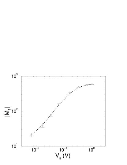
FIG. 1.: The amplitude $|M_{1}|$ of the output signal $v_{d}(t)$ at the frequency of the modulating signal as a function of the amplitude of the modulating signal $V_{s}$. The noise level $V_{rms}$ and the frequency of the modulating signal $f_{s}$ are kept constant at the values $V_{rms}=1.89$ V and $f_{s}=10$ Hz. A linear relation between $|M_{1}|$ and $V_{s}$ is detected within the interval $0.017\leq V_{s}\leq 0.067$.

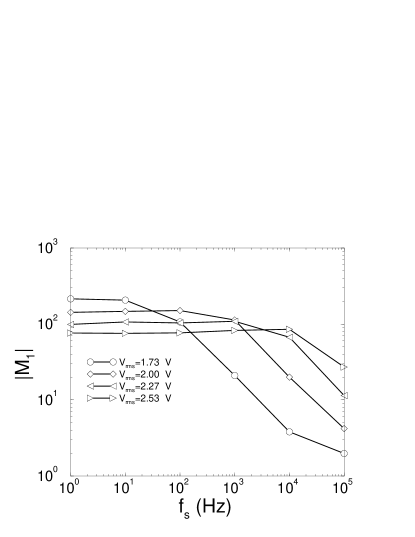
FIG. 2.: The amplitude $|M_{1}|$ of the output signal $v_{d}(t)$ at the frequency of the modulating signal as a function of the frequency of the modulating signal $f_{s}$. The amplitude of the modulating signal $V_{s}$ is kept constant at the value $V_{s}=0.067$ V whereas the noise level takes four different values: 1.73, 2.00, 2.27 and 2.53 V. For each value of the noise amplitude $|M_{1}|$ presents two regimes. An almost constant regime for $f<<\lambda_{min}/2\pi$ and a power-law decreasing regime (with exponent approximately -1.3) for $f>>\lambda_{min}/2\pi$. Experiments clearly show that $\lambda_{min}$ is controlled by the value of $V_{rms}$.

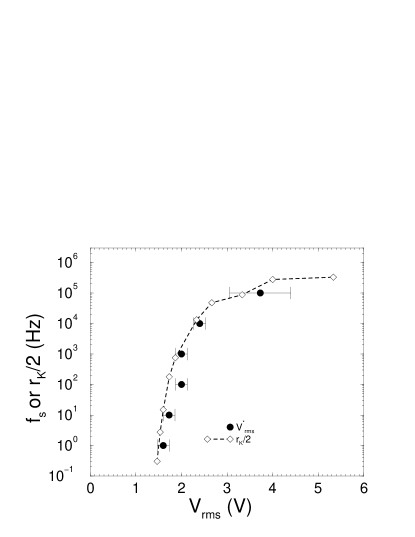
FIG. 3.: Comparison of (i) the occurrence of the maximal value of the $SNR$ (black circles) as a function of $V_{rms}$ and $f_{s}$ (error bars indicate the experimental uncertainty in the determination of the maximal $SNR$ with (ii) the experimental values of half of the Kramers rate $r_{k}/2$ observed in the same system in the absence of the modulating signal. In all the SR measurements the amplitude of the modulating signal is set to 0.067 V. The stochastic synchronization at the SR between half of the Kramers rate and the frequency of the modulating signal is experimentally observed in a frequency interval spanning 6 orders of magnitude

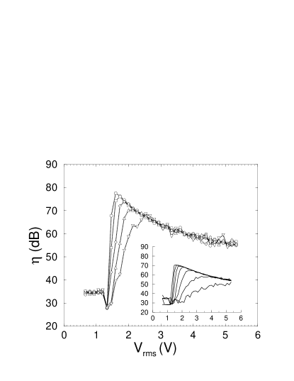
FIG. 4.: The amplitude $|M_{1}|$ of the output signal $v_{d}(t)$ at the frequency of the modulating signal as a function of the noise amplitude. The amplitude of the modulating signal $V_{s}$ is kept constant at the value $V_{s}=0.067$ V whereas the frequency takes five different values: 1 (circles), 10 (squares), 100 (diamonds), 1,000 (triangles up) and 10,000 (triangles down) Hz. The profile of $|M_{1}|$ becomes progressively more sharp as the frequency decreases. In the inset we show the result of the same kind of measurements performed in the nonlinear regime ($V_{s}=0.33$ V). In this case, higher values of the modulating frequency are investigated. Specifically the curves shown refer to values 1, 10, 100, 1,000, 10,000, 100,000 and 1,000,000 Hz, from top to bottom respectively. Also in this case the profile of $|M_{1}|$ becomes progressively more sharp as the frequency decreases but the low frequency limit is less sharp than expected from the linear response theory.

FIG. 5.: The amplitude $|M_{1}|$ of the output signal $v_{d}(t)$ at the frequency of the modulating signal as a function of the noise amplitude. The frequency of the modulating signal $f_{s}$ is kept constant at the value $f_{s}=10$ Hz whereas the amplitude takes eight different values 0.0067, 0.017, 0.033, 0.067, 0.167, 0.333, 0.667 and 1.00 V, which correspond to the lines shown from top to bottom respectively. By diminishing the amplitude $V_{s}$ the amplitude $|M_{1}|$ progressively approaches the limit predicted by the linear response theory. The convergence breaks down for low values of $V_{s}$ because for such a low level of $|M_{1}|$ the noise mask the presence of the signal. Hence the best approximation of a system evolving in the regime well described by the linear response theory is observed when $V_{s}=0.067$ V (fourth line starting from top).

FIG. 6.: Signal to Noise ratio (SNR) of the output signal $v_{d}(t)$ at the frequency of the modulating signal as a function of the noise amplitude. The frequency of the modulating signal $f_{s}$ is kept constant at the value $f_{s}=10$ Hz whereas the amplitude $V_{s}$ takes eight different values 0.0067, 0.017, 0.033, 0.067, 0.167, 0.333, 0.667 and 1.00 V, which correspond to the lines shown from bottom to top respectively. The customary general profile of the stochastic resonance is observed. However shape differences are observed by investigating the phenomenon at different values of $V_{s}$. Specifically, high values of $V_{s}$ (top curves) are characterized by distortions introduced by the active nonlinearities whereas at low values of $V_{s}$ (bottom curves) the SNR becomes negligible. As expressed in the caption of Fig. 5, the experimental condition better interpreted in terms of the linear response theory is the one observed for $V_{s}=0.067$ V (fourth line from bottom).

FIG. 7.: Noise level present in the output signal $v_{d}(t)$ at the frequency of the modulating signal as a function of the noise amplitude. The frequency of the modulating signal $f_{s}$ is kept constant at the value $f_{s}=10$ Hz whereas the amplitude $V_{s}$ takes eight different values 0.0067, 0.017, 0.033, 0.067, 0.167, 0.333, 0.667 and 1.00 V, which correspond to the lines shown from top to bottom respectively. By diminishing the amplitude $V_{s}$ the amplitude $|M_{1}|$ progressively approaches the curve observed in the absence of modulating signal (indeed the four curves with lowest values of $V_{s}$ are almost indistinguishable from the $V_{s}=0$ V observation). For the highest values of $V_{s}$ the presence of a dip is observed. The dip is more pronounced for higher value of $V_{s}$. When $V_{s}=0.667$ and $V_{s}=1.00$ V detailed structures emerge in the vicinity of the dip (see the inset for a blow-up of the region). These structures are responsible for the structure observed in the SNR near the maximum for highest values of $V_{s}$.

FIG. 8.: Time evolution of $v_{d}(t)$ measured in the nonlinear regime for three different values of the noise amplitude $V_{rms}$. All the time evolutions (top $V_{rms}=1.33$ V, middle up $V_{rms}=2.00$ V and middle down $V_{rms}=4.67$ V graph) are synchronously recorded with respect to the modulating signal (shown at the bottom of the figure).

REFERENCES

- [1] R. Benzi, A. Sutera, and A. Vulpiani, J. Phys. A 14, 453 (1981); R. Benzi, G. Parisi, A. Sutera, and A. Vulpiani, Tellus 34, 10 (1982).
- [2] L. Gammaitoni, P. Hänggi, P. Jung, and F. Marchesoni, Rev. Mod. Phys.70, 223 (1998).
- [3] C. R. Doering and J. C. Gadoua, Phys. Rev. Lett. 69, 2318 (1992).
- [4] C. Van den Broeck, J. M. R. Parrondo, and R. Torral, Phys. Rev. Lett. 73, 3395 (1994).
- [5] I. Dayan, M. Gitterman, and G. H. Weiss, Phys. Rev. A 46, 757 (1992).
- [6] R. N. Mantegna and B. Spagnolo, Phys. Rev. Lett. 76, 563 (1996).
- [7] K. Wiesenfeld, and F. Moss, Nature 33, 373 (1995)
- [8] B. McNamara, K. Wiesenfeld, and R. Roy, Phys. Rev. Lett.60, 2626 (1988).
- [9] R. N. Mantegna and B. Spagnolo, Phys. Rev. E 49, R1792 (1994).
- [10] B. McNamara and K. Wiesenfeld, Phys. Rev. A 39, 4854 (1989).
- [11] R. N. Mantegna and B. Spagnolo, Nuovo Cimento D 17, 873 (1995).
- [12] G. Giacomelli, F. Marin, and I. Rabbiosi, Phys. Rev. Lett.82, 675 (1999).
- [13] R. Landauer, J. Appl. Phys.33, 2209 (1962).
- [14] R. Landauer, Phys. Today 31, 23 (1978).
- [15] P. Hänggi and H. Thomas, Phys. Rep. 88, 207 (1982).
- [16] E. Lanzara, R. N. Mantegna, B. Spagnolo and R. Zangara, Am. J. Phys. 65, 341 (1997).
- [17] P. Jung and P. Hänggi, Phys. Rev. A 44, 8032 (1991).
- [18] V. A. Sneidman, P. Jung and P. Hänggi, Phys. Rev. Lett.72, 2682 (1994).
- [19] N. G. Stocks, Nuovo Cimento D 17, 925 (1995).
- [20] J.A. Freund, A. Neiman, and L. Schimansky-Geier, ’Stochastic Resonance and Noise-Induced Phase Coherence’, (pre-print).