Conductance fluctuations in diffusive rings:
Berry phase effects and criteria for adiabaticity

Abstract

We study Berry phase effects on conductance properties of diffusive mesoscopic conductors, which are caused by an electron spin moving through an orientationally inhomogeneous magnetic field. Extending previous work, we start with an exact, i.e. not assuming adiabaticity, calculation of the universal conductance fluctuations in a diffusive ring within the weak localization regime, based on a differential equation which we derive for the diffuson in the presence of Zeeman coupling to a magnetic field texture. We calculate the field strength required for adiabaticity and show that this strength is reduced by the diffusive motion. We demonstrate that not only the phases but also the amplitudes of the $h/2e$ Aharonov-Bohm oscillations are strongly affected by the Berry phase. In particular, we show that these amplitudes are completely suppressed at certain magic tilt angles of the external fields, and thereby provide a useful criterion for experimental searches. We also discuss Berry phase-like effects resulting from spin-orbit interaction in diffusive conductors and derive exact formulas for both magnetoconductance and conductance fluctuations. We discuss the power spectra of the magnetoconductance and the conductance fluctuations for inhomogeneous magnetic fields and for spin-orbit interaction.

I Introduction and Overview

Since its discovery, the Berry phase[1] has been a subject of continued interest. As this geometrical phase emerges from the very basic laws of quantum mechanics, it has implications for a broad range of physical systems.[2] Even though the Berry phase has been observed in single-particle experiments, its manifestation in condensed matter systems is still under investigation. Some settings were proposed, [3, 4, 5, 6, 7] where the Berry phase, resulting from the motion of a spin-carrying particle through an inhomogeneous magnetic field ${\mathbf{B}}({\mathbf{x}})$, can be observed in mesoscopic structures. The expected effects are measurable as persistent currents [3, 5, 8] as well as in the magnetoconductance[4, 6, 9, 10, 11] and the universal conductance fluctuations (UCFs).[4, 6] The first experiments reporting such effects were realized with semiconductor structures: the conductance was investigated in an InAs sample,[12] where the Berry phase can emerge through the Rashba effect[13], in a very similar way as produced by an inhomogeneous field. Magnetoconductance measurements were performed where a ferromagnetic dot, placed slightly above a GaAs sample, produced an inhomogeneous field.[14] Measurements on metallic systems also showed effects, which have been explained in terms of the Berry phase.[15, 16, 17] Further experiments on metallic systems are in progress.[18] An additional scenario was proposed, where domain walls of mesoscopic ferromagnets lead to a Berry phase.[7]

During orbital motion in a magnetic field, a spin acquires a Berry phase in a similar way as a charge collects an Aharonov-Bohm phase. Thus, these two phases lead to similar implications for interference phenomena in mesoscopic samples. However, in the first case the phase originates from the change in local field direction, whereas in the second case it results from an enclosed magnetic flux. As these field properties can be varied individually, the interplay of the two phases yields a rich variety of behaviour. These quantum phases are distinguished by another important difference: while Aharonov-Bohm effects appear for arbitrarily small magnitudes $B$ of the magnetic field, Berry phase effects appear to their full extent only in the adiabatic limit, i.e. for large enough fields (specified below). The physical situation required for this limit to be satisfied can be pictured [6, 11] as a spin which must complete many precessions ${\omega_{\rm B}}t_{o}/2\pi$ around the local magnetic field, while it moves during a time $t_{o}$ through a region of size $\ell_{B}$ over which the direction of the field changes significantly. Here we have introduced the Bohr frequency ${\omega_{\rm B}}=g{\mu_{\rm B}}B/2\hbar$, where $g$ is the Landé g-factor and ${\mu_{\rm B}}$ is the Bohr magneton. For ballistic motion as it occurs in clean semiconductors, one has ${v_{\rm F}}t_{o}\sim\ell_{B}$ and there is general consensus about the criterion for adiabaticity, i.e. ${\omega_{\rm B}}\ell_{B}/{v_{\rm F}}\gg 2\pi$, with ${v_{\rm F}}$ being the Fermi velocity. However, for diffusive systems there were recently some discussions[9, 6, 10, 11] whether $t_{o}$ can be correctly set as the diffusion time $t_{d}=\ell_{B}^{2}/D$ or if one should replace it by the elastic scattering time $\tau$. The first criterion is more optimistic, in the sense that much lower field magnitudes are required to reach adiabaticity, as due to diffusive motion the electrons effectively move more slowly (compared to the ballistic motion) through the changing magnetic field and thus have more time to adjust their spins to the local field orientation. For magnetoconductance quantitative values for the required field magnitudes have been obtained.[11] Solving the special case of a cylindrically symmetrical texture exactly, it was confirmed [11] that the more favorable criterion is indeed sufficient. We remark that, if the ballistic criterion was appropriate for diffusive systems, the large fields required for adiabaticity would imply a strong curvature of the semiclassical trajectories (apart from the case of very large $g$ factors). This curvature in turn is in conflict with the approximation of the orbital motion by its zero-field value and therefore an approach beyond weak localization theory would be required for a self-consistent theory. At this point it should also be noted that Berry phase effects occur even if the adiabatic limit is not fully reached; there is no sharp cutoff where the Berry phase disappears completely. Thus, calculations without assuming adiabaticity are very desirable, as they can be used to study how the Berry phase effects gradually emerge while the magnetic field is increased from low to adiabatic strengths. The adiabatic limit can still be taken at the end of the calculation, so the formal appearance of the Berry phase and the associated dephasing[11] can be identified.

Besides having a spin following the direction of an inhomogeneous external field, there is another scenario which produces a Berry phase: spin-orbit coupling.[13] If an electron moves through an electrical field perpendicular to the ring plane, an effective magnetic field, which is produced in the rest frame of the electron, couples to the electron spin. As this effective field is in radial direction of the ring and perpendicular to the direction of motion, the field rotates while the electron moves around the ring and can therefore produce a Berry phase. By switching on, in addition, an external magnetic field, an arbitrary tilt angle of the total effective field can be realized and so this Berry phase can be tuned. For ballistic motion, the Berry phase manifests itself in precisely the same way [13] as in the case with an inhomogeneous external magnetic field.[3, 4, 5] However, for diffusive motion the situation becomes more complicated, as the change of the direction of motion of the electron due to a elastic scattering event abruptly changes the effective field direction. Now the picture of a spin, moving adiabatically through a slowly varying field, is no longer valid and needs to be modified. This leads to a new physical situation which has to be considered separately from the situation with inhomogeneous fields.

The outline of this paper is as follows. In Sec. II we study the conductance fluctuations $\delta g^{(2)}$ of quasi-1D diffusive rings in inhomogeneous magnetic fields. While $\delta g^{(2)}$ has already been calculated within the adiabatic approximation,[6] i.e. for strong magnetic fields, the behavior outside the adiabatic limit and the influence of inhomogeneous fields on dephasing were not dicussed so far. We address these issues in the present work, starting in Sec. II A with a calculation of an exact expression for $\delta g^{(2)}$ (i.e. allowing arbitrarily small field magnitudes) for a special texture [see Eq. (1)] of the magnetic field. In this process we derive a new form of the diffuson differential equation, which includes inhomogeneous magnetic fields. We evaluate the adiabatic limit of the UCFs, $\delta g^{(2)}_{\rm ad}$, in Sec. II B and compare our results with those derived in previous work.[6] Further, we investigate in Sec. II C the finite temperature behavior of the conductance fluctuations. In Sec. III the effects of the Berry phase on the UCFs and their dependence on magnetic field strengths are discussed in detail. We identify in Sec. III A a new effect of the Berry phase by showing that the amplitudes of the $h/2e$ Aharonov-Bohm oscillations depend directly on the value of the Berry phase. In particular, we find some magic tilt angles of the magnetic field, where these Aharonov-Bohm oscillations are completely suppressed. This effect provides a tool for experimental searches of the Berry phase. We use this observation to illustrate the gradually appearing effects of the Berry phase for increasing field strengths and thus give a direct demonstration of the onset of adiabaticity. Then, in Sec. III B, we give quantitative values of the fields strengths needed for reaching adiabaticity. We show that the criterion for adiabaticity is less stringent for diffusive than for ballistic motion. An exact evaluation of magnetoconductance $\delta g_{\scriptscriptstyle\mathit{S}O}$ and conductance fluctuations $\delta g^{(2)}_{\scriptscriptstyle\mathit{S}O}$ in the presence of spin-orbit coupling and homogeneous magnetic fields is given in Sec. IV. These results show how the amplitudes of the Aharonov-Bohm oscillations in $\delta g^{(2)}_{\scriptscriptstyle\mathit{S}O}$ depend non-monotoneously on the direction of an effective field, similarly as it is the case for inhomogeneous magnetic fields. In Sec. V A we show how frequency shift of the Aharonov-Bohm oscillations appear in $\delta g$ and $\delta g^{(2)}$ caused by the Berry phase. We then point out in Sec. V B that the Zeeman term can also produce frequency shifts even in the case of homogeneous fields. In Sec. V C we plot and discuss the exact expressions for $\delta g$ and $\delta g^{(2)}$ for inhomogeneous fields and for spin-orbit coupling as well as the corresponding power spectra. In three appendices we provide details of our calculations.

II Conductance Fluctuations

As foundation for further discussions of Berry phase effects and adiabaticity, we will first calculate the conductance fluctuations $\delta g^{(2)}$ in the weak-localization regime. To motivate the analysis of the conductance fluctuations, we would like to emphasize the advantage of studying the UCFs instead of the magnetoconductance. The latter quantity has only contributions from the cooperon, which are suppressed by moderately large magnetic fields penetrating the ring arms.[19] This suppression is in direct competition with the requirement of having large fields to satisfy adiabaticity. In contrast, the conductance fluctuations also have contributions from the diffuson, which is only sensitive to the difference of the two magnetic fields, for which the conductance correlator is considered. Therefore, if both fields are taken of similar magnitude, Aharonov-Bohm oscillations and Berry phase effects in the UCFs will still be visible at high magnetic fields where the adiabatic criterion is certainly satisfied.

A Exact solution

We shall concentrate on rings with circumference $L$ and study the conductance-conductance correlator $\delta g^{(2)}({\mathbf{B}},{\mathbf{\tilde{}}{B}})=\left\langle g_{\raisebox{-1.50694pt}{$\scriptstyle{\mathbf{B}}$}}g_{\raisebox{-1.50694pt}{$\scriptstyle{\mathbf{\tilde{}}{B}}$}}\right\rangle-\left\langle g_{\raisebox{-1.50694pt}{$\scriptstyle{\mathbf{B}}$}}\right\rangle\left\langle g_{\raisebox{-1.50694pt}{$\scriptstyle{\mathbf{\tilde{}}{B}}$}}\right\rangle$, where we have two different magnetic fields ${\mathbf{B}}$ and ${\mathbf{\tilde{}}{B}}$. We consider a special texture[5, 10, 11] for which we obtain exact results (i.e. without making the adiabatic assumption of strong magnetic fields). We assume the magnetic fields to be applied in such a way that they wind $f$ times around the $z$-axis in one turn around the ring, with tilt angles $\eta$, $\tilde{\eta}$, see Fig. 1. The position along the direction of the ring is described by the coordinate $x$, varying from $0$ to $L$, so the special texture of the magnetic field is expressed as

$${\mathbf{B}} = B\,{\mathbf{n}}$$ (1)

$$= B\,(\sin{\eta}\,\cos{\textstyle(\frac{2\pi fx}{L}\!+\!\theta)},\,\sin{\eta}\,\sin{\textstyle(\frac{2\pi fx}{L}\!+\!\theta)},\,\cos{\eta}),$$ (2)

and similarly for ${\mathbf{\tilde{}}{B}}$. We have introduced $\theta$, so we can describe the textures with a field component radial to the ring, i.e. $\theta=0$, as well as textures with a field component tangential to the ring, i.e. $\theta=\pi/2$.

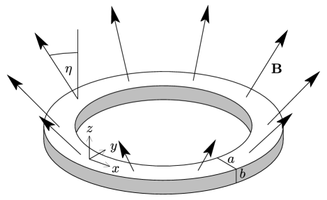
FIG. 1.: A mesoscopic ring of width $a$ and height $b$ in an inhomogeneous magnetic field with tilt angle $\eta$, winding once around the $z$-Axis. The texture of the magnetic field drawn here corresponds to Eq. (1) with $f=1$ and $\theta=0$.

The starting point of our calculation is the conductance correlator derived in Ref. [6] and given by

$$\delta g^{(2)} = \left(\frac{2e^{2}D}{hL^{2}}\right)^{2}\int d\epsilon\,d\epsilon^{\prime}n^{\prime}(\epsilon)\,n^{\prime}(\epsilon^{\prime})\left\{\frac{1}{d}{\rm Tr}\,\hat{\chi}^{C}_{\omega}\hat{\chi}^{C\dagger}_{\omega}\right.$$ (4)

$$\left.+2\,{\rm Re}\,{\rm Tr}\,\hat{\chi}^{C}_{\omega}\hat{\chi}^{C}_{\omega}+\left[\hat{\chi}^{C}\rightarrow\hat{\chi}^{D}\right]\right\},$$

where $n^{\prime}(\epsilon)$ is the derivative of the Fermi function and $\hbar\omega=\epsilon-\epsilon^{\prime}$. The dimensionality of the system with respect to the diffusive motion is denoted by $d$, which describes the relation of the mean free path $\ell$ to the diffusion coefficient $D$, i.e. $D={v_{\rm F}}\ell/d$. The propagators $\hat{\chi}^{C/D}$ can be evaluated explicitly by using the operator equation Eq. (A10):

$$\hat{\chi}^{C/D}=\frac{L^{2}}{(2\pi)^{2}D}\>\frac{1}{iw+\gamma^{C/D}-h^{C/D}}.$$ (5)

We have defined $w=(L/2\pi L_{T})^{2}\,(\epsilon-\epsilon^{\prime})/kT$, with the thermal diffusion length $L_{T}=\sqrt{D\hbar\beta}.$[20] The (non-hermitian) Hamiltonian is given by

$$h^{C/D}=\frac{L^{2}}{(2\pi)^{2}}\frac{\partial^{2}}{\partial x^{2}}+i\kappa{\mathbf{n}}\cdot\mbox{\boldmath{$\sigma$}}_{1}-i\tilde{\kappa}{\mathbf{\tilde{}}{n}}\cdot\mbox{\boldmath{$\sigma$}}_{2}^{(*)},$$ (6)

where the star means complex conjugation in $h^{D}$ and where we have introduced an adiabaticity parameter [6, 11, 10]

$$\kappa=\frac{{\omega_{\rm B}}}{D}\frac{L^{2}}{(2\pi)^{2}},$$ (7)

and equivalently for $\tilde{\kappa}$ and ${\omega_{\tilde{\rm B}}}$. We have inserted a phenomenological damping constant $\gamma^{C/D}=(L/2\pi L_{C/D})^{2}$ expressed in terms of the magnetic dephasing length $L_{C/D}$[19, 6]:

$$\gamma^{C/D}=\frac{L^{2}}{(2\pi)^{2}L_{\varphi}^{2}}+\frac{1}{3(4\pi)^{2}}\left(\frac{A\,|B_{z}\pm\tilde{B}_{z}|}{2\pi\phi_{0}}\right)^{2}.$$ (8)

The first term of this damping constant incorporates the loss of phase due to inelastic scattering events. The second term takes into account magnetic flux penetration into the arms of the ring with a finite width $a$ and a surface area $A=aL$, while the height $b$ is assumed to be small compared to $a$. This field penetration leads to averaging over closed paths of different lengths, each of which collects a different Aharonov-Bohm phase, resulting finally in dephasing.

Next we define the basis in which we evaluate the Hamiltonian $h^{C/D}$. As done in Ref. [10] for the cooperon propagator, we now introduce the operators

$$J^{C/D}=\frac{L}{2\pi i}\frac{\partial}{\partial x}+\frac{1}{2}f(\sigma_{1z}\pm\sigma_{2z}),$$ (9)

which commute with $h^{C/D}$.[21]

We will now go to the basis of eigenvectors $\left|j,\alpha\beta\right\rangle_{C/D}$ of $J^{C/D}$. This basis is orthonormal with the following wave functions:

$$\left\langle x,\alpha^{\prime}\beta^{\prime}|j,\alpha\beta\right\rangle_{C/D}=\frac{\delta_{\alpha^{\prime}\alpha}\delta_{\beta^{\prime}\beta}}{\sqrt{L}}\;\exp\left\{{\textstyle\frac{2\pi ix}{L}(j-\frac{f}{2}\alpha\mp\frac{f}{2}\beta)}\right\}.$$ (10)

Because of the periodic boundary conditions in $x$, the eigenvalues $j$ of $J^{C/D}$ have to be integers. The matrix elements of $h^{C/D}$ in the basis $\{\left|j,\uparrow\uparrow\right\rangle_{C/D},\left|j,\uparrow\downarrow\right\rangle_{C/D},\left|j,\downarrow\uparrow\right\rangle_{C/D},\left|j,\downarrow\downarrow\right\rangle_{C/D}\}$ become:

$$_{C/D}\!\left\langle j,\alpha\beta\left|h^{C/D}\right|j^{\prime},\alpha^{\prime}\beta^{\prime}\right\rangle{}_{C/D}=\delta_{jj^{\prime}}\left(-h_{j}^{C/D}+h_{\sigma}^{C/D}\right),$$ (11)

where $h_{j}^{C}$ and $h_{j}^{D}$ are diagonal 4$\times$4 matrices with the entries $\{(j-f)^{2},j^{2},j^{2},(j+f)^{2}\}$, and $\{j^{2},(j-f)^{2},(j+f)^{2},j^{2}\}$, resp., and the $\eta$, $\tilde{\eta}$ dependent matrices are

$$h_{\sigma}^{C/D}=\left(\begin{array}[]{*{3}{c@{\!}}c}i\kappa\,\cos{\eta}-i\tilde{\kappa}\,\cos{\tilde{\eta}}&-i\tilde{\kappa}e^{\mp i\theta}\,\sin{\tilde{\eta}}&i\kappa e^{-i\theta}\,\sin{\eta}&0\\ -i\tilde{\kappa}e^{\pm i\theta}\,\sin{\tilde{\eta}}&i\kappa\,\cos{\eta}+i\tilde{\kappa}\,\cos{\tilde{\eta}}&0&i\kappa e^{-i\theta}\,\sin{\eta}\\ i\kappa e^{i\theta}\,\sin{\eta}&0&-i\kappa\,\cos{\eta}-i\tilde{\kappa}\,\cos{\tilde{\eta}}&-i\tilde{\kappa}e^{\mp i\theta}\,\sin{\tilde{\eta}}\\ 0&i\kappa e^{i\theta}\,\sin{\eta}&-i\tilde{\kappa}e^{\pm i\theta}\,\sin{\tilde{\eta}}&-i\kappa\,\cos{\eta}+i\tilde{\kappa}\,\cos{\tilde{\eta}}\end{array}\right).$$ (12)

To take the Aharonov-Bohm flux into account, we replace $j\rightarrow m=j-(\phi/\phi_{0}\pm\tilde{\phi}/\phi_{0})$, where $\phi,\tilde{\phi}$ are the fluxes of the fields ${\mathbf{B}},{\mathbf{\tilde{}}{B}}$ through the ring and $\phi_{0}=h/e$ is the magnetic flux quantum.[22] Now it is straightforward to evaluate the exact conductance fluctuations $\delta g^{(2)}$ by calculating the propagators by matrix inversion and inserting the result into Eq. (4). This can be done with the help of the computer program Mathematica, which however leads to lengthy expressions which we will not reproduce here. We merely point out that the phase factors in $\theta$ cancel each other in $\delta g^{(2)}$ and $\delta g$.

B Adiabatic Approximation

To evaluate the adiabatic limit, we shall consider the regime of large magnetic fields with $B$ and $\tilde{B}$ of similar magnitude. If we define $\Delta\kappa=\tilde{\kappa}-\kappa$, this adiabatic regime is described by

$$\kappa\gg 1\quad\mbox{and}\quad\kappa\gg|\Delta\kappa|.$$ (13)

The exact propagators $\chi^{C/D}$ turn out to be rational functions which are of order two in $\kappa$ in both numerator and denominator. Now we will keep only the terms of highest order in $\kappa$; terms with large $j$ can be neglected as the sum over $j$ converges rapidly. This leads us to the UCFs in the adiabatic regime:

$$\delta g^{(2)}_{\rm ad} = \left(\frac{e^{2}}{h}\right)^{2}\frac{1}{4\pi^{4}}\int d\epsilon\,d\epsilon^{\prime}n^{\prime}(\epsilon)\,n^{\prime}(\epsilon^{\prime})\sum_{j=-\infty}^{\infty}\sum_{\alpha=\pm 1}\left(G^{\rm ad}_{\alpha,C}+G^{\rm ad}_{\alpha,D}\right)$$ (14)

$$G^{\rm ad}_{\alpha,C/D} = \frac{1}{d}\left\{{{\left(w-\alpha\Delta\kappa\right)}^{2}}+{\delta^{C/D}_{-\alpha}(j)}^{2}+P\right\}\times\left\{\left[{{\left(w-\alpha\Delta\kappa\right)}^{2}}+{\delta^{C/D}_{-\alpha}(j)}^{2}-P\right]\right.$$ (16)

$$\qquad\left.\cdot\left[{{\left(w+\alpha\Delta\kappa\right)}^{2}}+{\delta^{C/D}_{\alpha}(j)}^{2}-P\right]+4P\left[{w^{2}}+f^{2}m^{2}\left(\cos{\eta}\pm\cos{\tilde{\eta}}\right)^{2}\right]\right\}^{-1}$$

$$+ 2{\rm Re}\bigglb[\left\{\left[iw-i\alpha\Delta\kappa+{\delta^{C/D}_{-\alpha}(j)}\right]^{2}+P\right\}$$ (18)

$$\times\left\{\left[iw-i\alpha\Delta\kappa+{\delta^{C/D}_{-\alpha}(j)}\right]\left[iw+i\alpha\Delta\kappa+{\delta^{C/D}_{\alpha}(j)}\right]-P\right\}^{-2}\biggrb],$$

where

$$P = \frac{f^{4}}{4}\,\sin^{2}{\eta}\,\sin^{2}{\tilde{\eta}},$$ (19)

$${\delta^{C/D}_{\alpha}(j)} = \tilde{\gamma}^{C/D}_{\eta,\,\tilde{\eta}}+\left(m-\frac{f}{2}\,\alpha\,\cos{\eta}\mp\frac{f}{2}\,\alpha\,\cos{\tilde{\eta}}\right)^{2},$$ (20)

with

$$\tilde{\gamma}^{C/D}_{\eta,\,\tilde{\eta}} = \gamma^{C/D}+\frac{f^{2}}{4}\,\sin^{2}{\eta}+\frac{f^{2}}{4}\,\sin^{2}{\tilde{\eta}}.$$ (21)

The sum over $\alpha$ has been introduced here artificially to facilitate the following interpretation. As it is also seen in Ref. [11] for the case of the magnetoconductance $\delta g$, the terms $f^{2}(\sin^{2}{\eta}+\sin^{2}{\tilde{\eta}})/4$ in Eq. (21) act as additional dephasing sources and are here absorbed in the phenomenological dephasing parameter $\tilde{\gamma}^{C/D}_{\eta,\,\tilde{\eta}}$. However, in Eq. (18) there are further $\eta$, $\tilde{\eta}$-dependent terms $P$, which cannot be formally absorbed in $\tilde{\gamma}^{C/D}_{\eta,\,\tilde{\eta}}$. $P$ reduces the effect of the additional dephasing terms in Eq. (21), as we can see by the following numerical evaluation. We consider equal fields ${\mathbf{B}}={\mathbf{\tilde{}}{B}}$ and low temperatures, thus $\Delta\kappa,\,\omega=0$, and assume $\eta$, $\tilde{\eta}$ to be close to $\pi/2$. Then we estimate the amplitude of the Aharonov-Bohm oscillations by taking the difference between the values of $G^{\rm ad}_{\alpha,C}$ [Eq. (18)] for the two phases $m=0$ and $m=\pm 1/2$ (i.e. we are considering only the main contributions in the sum over $j$ [Eq. (14)]). We then see by numerical evaluation that the oscillations are suppressed if we set $P=0$ instead of using Eq. (19), thus $P$ indeed reduces dephasing.

We can compare now with previous calculations[6] where the UCFs $\delta g^{(2)}_{\rm LSG}$ have been derived for arbitrary textures and adiabatic evolution of the spin. These results can be recovered from Eq. (14) by the replacement $\tilde{\gamma}^{C/D}_{\eta,\,\tilde{\eta}}\to\gamma^{C/D}_{\rm LSG}$ and $P\to 0$. The dephasing terms due to inhomogeneous fields coupling to the spin [see Eqs. (19), (21)] were not explicitly given in Ref. [6]; to account for such dephasing these terms must be included in the phenomenological parameter $\gamma^{C/D}_{\rm LSG}$, and thus $\gamma^{C/D}_{\rm LSG}\neq\gamma^{C/D}$ and $\gamma^{C/D}_{\rm LSG}\neq\tilde{\gamma}^{C/D}_{\eta,\,\tilde{\eta}}$ in general.[11]

We also recognize a strong simplification in the special case where one field is homogeneous, $\eta=0$, i.e., $P$ vanishes. Thus the comparison of $\delta g^{(2)}_{\rm ad}$ with the solution for arbitrary textures $\delta g^{(2)}_{\rm LSG}$ yields the simple relation $\gamma^{C/D}_{\rm LSG}=\tilde{\gamma}^{C/D}_{0,\,\tilde{\eta}}$. Finally we note that in this case the dephasing due to the orientational inhomogenity of ${\mathbf{\tilde{}}{B}}$ measured by the winding $f$ grows like $f^{2}\,\sin^{2}{\tilde{\eta}}$ [cf. Eq. (21)].

C Finite Temperatures

Now we consider the effects of finite temperatures $T\!>\!0$ on the UCFs $\delta g^{(2)}_{\rm ad}$ in the adiabatic regime. In the case of $\eta=0$, i.e. $P=0$, the factors containing ${\delta^{C/D}_{-\alpha}(j)}$ in Eq. (18) cancel, so we obtain

$$\left.G^{\rm ad}_{\alpha,C/D}\right|_{\eta=0} = \frac{1}{d}\left\{{{\left(w+\alpha\Delta\kappa\right)}^{2}}+{\delta^{C/D}_{\alpha}(j)}^{2}\right\}^{-1}$$ (23)

$$+2{\rm Re}\left\{iw+i\alpha\Delta\kappa+{\delta^{C/D}_{\alpha}(j)}\right\}^{-2}.$$

This strong simplification allows us to evaluate the integrals over $\epsilon$ and $\epsilon^{\prime}$ in Eq. (14) explicitly by using standard Matsubara techniques, as described in App. B, and we obtain for the UCFs $\delta g^{(2)}_{\rm ad}=\delta g^{(2)}_{{\rm ad},\,C}+\delta g^{(2)}_{{\rm ad},\,D}$,

$$\left.\delta g^{(2)}_{{\rm ad},\,C/D}\right|_{\eta=0} =\!\left(\frac{e^{2}}{h}\right)^{2}\!\!\frac{1}{8\pi^{6}}\left(\frac{L^{2}}{L_{T}^{2}}\right)^{2}{\rm Re}\sum_{\alpha=\pm 1}\left.\sum_{j,n,m}\right.^{\prime}$$ (26)

$$\!\!\!\!\!\!\!\!\left\{\frac{1}{d\,\delta_{\alpha}^{C/D}(j)\cdot\left[\frac{L^{2}}{4\pi L_{T}^{2}}(m\!+\!n)\!+\!\delta_{\alpha}^{C/D}(j)\!-\!i\alpha\Delta\kappa\right]^{3}}\right.$$

$$\left.+\frac{6}{\left[\frac{L^{2}}{4\pi L_{T}^{2}}(m\!+\!n)\!+\!\delta_{\alpha}^{C/D}(j)\!-\!i\alpha\Delta\kappa\right]^{4}}\right\}.$$

Here $n$ and $m$ are odd, positive integers. For plotting, it is advantageous to calculate the sum in Eq. (26) analytically, which gives an expression containing Psi-functions.

We can now obtain a qualitative criterion when the thermal dephasing effects can be ignored. If we ignore thermal effects, i.e. assume low temperatures, we can simplify our calculation leading to Eq. (26) by replacing $n^{\prime}(\epsilon)$ by a delta function $\delta(\epsilon)$ in Eq. (14). This yields for $\eta=0$ the same result as applying Poisson’s summation formula to Eq. (26) in order to replace the summations over $n$ and $m$ by integrations. We are only allowed to perform this step if the summand varies slowly in $n$, $m$, which is the case for $L_{T}^{2}\gg 2\pi L_{C/D}^{2}$. From a physical point of view, this is an evident requirement: the smearing of the conductance fluctuations due to nonzero temperatures, described by the thermal diffusion length $L_{T}$, can only be neglected if the dephasing lengths related to inelastic scattering or penetrating magnetic fields are much shorter than $L_{T}$.

In App. C we evaluate the dephasing behavior of the UCFs $\delta g^{(2)}_{\rm hom}$ for homogeneous fields and finite temperatures. Then we confirm the result of Ref. [6] [Eq. (4)] and show that our calculation in the homogeneous limit indeed reproduces known results.[20, 23, 24]

III Berry phase and Adiabaticity

A Magic Angles—Qualitative Criterion for Adiabaticity

We now consider the qualitative effects of the Berry phase on the conductance fluctuations $\delta g^{(2)}$. They emerge from the Berry phase in ${\delta^{C/D}_{\alpha}(j)}$ in the adiabatic solution [Eq. (14)] and lead to vanishing Aharonov-Bohm oscillations at special “magic” tilt angles of the magnetic fields. This effect has some similarities with the phenomenon of beating, where the superposition of two oscillations with different but fixed frequencies leads to a periodic vanishing of the envelope. However, in our case we have two frequencies which will change when the perpendicular field $B_{z}$ is increased, since then the Berry phase is altered, too. Thus a suppression of the Aharonov-Bohm oscillations can only be observed at two special tilt angles of the magnetic field, i.e. the Berry phase has a highly non-periodic effect on the envelope of these oscillations as a function of $B_{z}$.

From now on we shall only study the experimentally realizable field texture with one winding, $f=1$. The other configurations with $f>1$ are solely of academic interest. To illustrate expected experimental results, we will use some material parameters recently determined.[25] The sample Au-1 given in Table I of Ref. [25] has the values $D=9\times 10^{-3}\>{\rm m}^{2}\,{\rm s}^{-1}$ and $L_{\varphi}=\sqrt{D\tau_{\varphi}}=5.54\>\mu{\rm m}$. We assume a ring with diameter of $4\>\mu{\rm m}$, so $L=12.6\>\mu{\rm m}$, and an arm width $a=60\,{\rm nm}$, which lies well within present-day experimental reach. Finally we assume low temperatures, i.e. $L_{T}\gg L,L_{\varphi}$, so we can ignore the dephasing due to thermal fluctuations.

Now we shall consider two equal fields, so no phase terms appear in the diffuson contribution $\delta g^{(2)}_{D}$. The cooperon contribution $\delta g^{(2)}_{C}$ is $h/2e$ periodic in the magnetic flux, as a shift of $m=\phi/\phi_{0}+\tilde{\phi}/\phi_{0}+j=2\phi/\phi_{0}+j$ by 1 is absorbed in the sum over $j$ in Eq. (14). For the next argument we take the dephasing due to inhomogeneous fields only phenomenologically into account, i.e. we use the result $\delta g^{(2)}_{\rm LSG}$ from Ref. [6] or equivalently set $P=0$ [Eqs. (14, 23)], so the factors containing ${\delta^{C/D}_{-\alpha}(j)}$ cancel in Eq. (18). If the tilt angle $\eta$ is such that $\cos{\eta}=1/4$, the phase dependent term in ${\delta^{C/D}_{\alpha}(j)}$ [Eq. (20)] becomes $m-\alpha/4$. One sees that in this special case shifting $m$ by $1/2$ does not affect the value of $\delta g^{(2)}_{C}$, as it leads solely to an exchange $\alpha\to-\alpha$. The very same argument applies to $\cos{\eta}=3/4$. Thus, for these magic angles $\eta$, where $\cos{\eta}=1/4,3/4$, the UCFs $\delta g^{(2)}$ are $h/4e$ periodic and therefore their power spectrum shows a vanishing $h/2e$ amplitude. If we take the exact solution in the adiabatic regime $\delta g^{(2)}_{\rm ad}$ instead of $\delta g^{(2)}_{\rm LSG}$, the magic angles are still present, but at shifted values. The angle at $\cos{\eta}=3/4$ is nearly unaffected, as $P\approx 0.05$ is very small at this angle. The suppression of the Aharonov-Bohm oscillations is illustrated in Fig. 2 (see also Sec. V C and Fig. 9) by plotting the $h/2e$ amplitude of the exact solution $\delta g^{(2)}$ with varying tilt angle $\eta$ and for different radial field components. As one can readily see from Fig. 2, the effect described here is fully developed for $B\geq 200\>{\rm G}$. For smaller fields, the $h/2e$ amplitude does not completely vanish at the magic angles, as adiabaticity is not yet reached. It should be noted that even if the adiabatic regime is not fully reached, an effect of the Berry phase is still visible as a distinct non-monotonic behavior of the UCFs $\delta g^{(2)}$ as a function of the tilt angle $\eta$, unlike the UCFs for a configuration with a homogeneous field texture (also shown in Fig. 2).

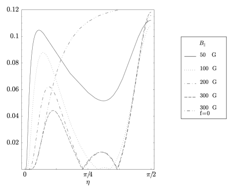
FIG. 2.: The normalized amplitudes of the $h/2e$ oscillations in the UCFs $\delta g^{(2)}$, as a function of the tilt angle $\eta$. The magnetic fields are chosen equal, i.e. ${\mathbf{B}}={\mathbf{\tilde{}}{B}}$, and wind once around the ring (i.e. $f=1$). The power spectrum of the exact UCFs $\delta g^{(2)}$ has been calculated at every tilt angle $\eta$ by varying the Aharonov-Bohm flux $0\leq\phi=\tilde{\phi}\leq 1$. The component of the $h/2e$ oscillation in this spectrum was then normalized by the 0th order Fourier component and is plotted here as a function of $\eta$. Four configurations of radial fields $B_{||}=\tilde{B}_{||}$ are shown; the perpendicular field components $B_{z}=\tilde{B}_{z}$ are determined by the tilt angles $\eta=\tilde{\eta}$. These field components and so also $\gamma^{C}$, as it depends on the arm-penetrating field, increase for small $\eta$. The strong dephasing $\gamma^{C}$ at $\eta\approx 0$ can be observed as vanishing oscillations. The most remarkable effects show up for the stronger fields $B_{||}=200\>{\rm G},\,300\>{\rm G}$ at the magic angles $\eta=0.72,\,1.15$. Here the Berry phase eliminates the $h/2e$ oscillations, as it is described in Section III A. For comparison, we also show the conductance fluctuations for a homogeneous field, i.e. setting $f=0$. We here set $T=0$ and used the material parameters $L=12.6\>\mu{\rm m}$, $a=60\,{\rm nm}$, $D=9\times 10^{-3}\>{\rm m}^{2}\,{\rm s}^{-1}$, and $L_{\varphi}=5.54\>\mu{\rm m}$.

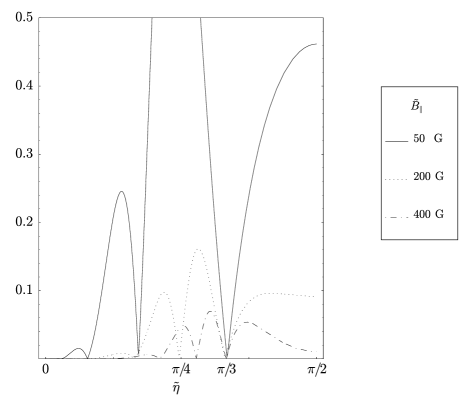
FIG. 3.: The normalized amplitudes of the $h/e$ oscillations in the UCFs $\delta g^{(2)}$, with $\eta=0$, as a function of the tilt angle $\tilde{\eta}$. The field were taken as ${\mathbf{B}}=(2/\sqrt{3})\tilde{B}_{\parallel}\,{\mathbf{e}}_{z}$, $\tilde{B}_{\parallel}={\rm const.}$, and $\tilde{B}_{z}$ was determined through the tilt angle $\tilde{\eta}$. We use the same methods and parameters as described in Fig. 2 for $\tilde{B}_{\parallel}=50\>{\rm G}$, $200\>{\rm G}$, and $400\>{\rm G}$. We notice that the $h/e$ oscillations become suppressed by the Berry phase at the magic angle $\cos{\tilde{\eta}}=\pi/3$.

Another interesting situation arises for $B\neq\tilde{B}$. Now, phase effects from the diffuson contribution to $\delta g^{(2)}$ emerge and remain present even for large fields, since the dephasing due to flux penetrating the arms of the ring depends only on the difference of the fields and not on the sum as for the cooperon contribution, see Eq. (8). For illustration, we consider the configuration where ${\mathbf{B}}$ is homogeneous with $\eta=0$. The other field ${\mathbf{\tilde{}}{B}}$ is assumed to have a radial component so that for a tilt angle $\tilde{\eta}=\pi/3$ the magnitudes of both fields are equal, i.e. $\tilde{B}_{||}=(\sqrt{3}/2)B_{z}$. In the adiabatic approximation $\delta g^{(2)}_{\rm ad}$ [Eq. (14)] $P$ vanishes, yielding the simple relation Eq. (21) between the dephasing due to the inhomogeneous field textures and $\gamma^{C/D}$: the effective dephasing will be increased by $3/16$ at the most interesting angle, $\tilde{\eta}=\pi/3$, in the situation considered here. The contribution of the penetrating fields to $\gamma^{C/D}$ will be three times larger for the cooperon than for the diffuson, as can be seen from Eq. (8). Varying $\tilde{B}_{z}$ changes the Aharonov-Bohm phase $\tilde{\phi}/\phi_{0}$, while $\phi/\phi_{0}={\rm const.}$, leading to $h/e$ oscillations. At $\tilde{B}_{z}=B_{z}/2$ two features are worth mentioning. First, the magnitudes of both fields become equal, therefore $\Delta\kappa$ vanishes and so the second part of the criterion in Eq. (13) is fulfilled and we can use the adiabatic approximation $\delta g^{(2)}_{\rm ad}$ [Eq. (14)]. Second, we have $\cos{\tilde{\eta}}=1/2$, so the phase dependent terms $m\mp\alpha/4$ arise in ${\delta^{C/D}_{\alpha}(j)}$, as can be seen from Eq. (20). With the same argument as above, the UCFs $\delta g^{(2)}$ become $h/2e$ periodic at this magic angle $\pi/3$, so the $h/e$ amplitude vanishes in the power spectrum. We note that, in the adiabatic regime, this magic angle is exact, since for the configuration $\eta=0$ we have $\delta g^{(2)}_{\rm ad}=\delta g^{(2)}_{\rm LSG}$. This is shown in Fig. 3, again as a function of the tilt angle $\tilde{\eta}=\cot{(\tilde{B}_{z}/B_{z})}$, see also Sec. V C and Fig. 10.

B Quantitative Criterion for Adiabaticity

In order to obtain a quantitative criterion for adiabaticity, we numerically compare the exact solution of the conductance fluctuations $\delta g^{(2)}$ with the adiabatic approximation $\delta g^{(2)}_{\rm ad}$ [Eq. (14)]. We take equal magnitudes for both fields, i.e. $B=\tilde{B}$. We search for a minimal $\kappa_{\rm min}$ so that the relative difference $\big{|}\delta g^{(2)}-\delta g^{(2)}_{\rm ad}\big{|}\big{/}\delta g^{(2)}$ is below a certain value. This is done with a bisection algorithm (in $\kappa$) and by sampling over the parameter subspace $[0,\pi/2]^{2}\times[0,1]^{2}\times[\frac{1}{100},10]^{2}\subset\{(\eta,\,\tilde{\eta},\,\phi/\phi_{0},\,\tilde{\phi}/\phi_{0},\,\gamma^{C},\,\gamma^{D})\}$ with a grid resolution of 10 intersections in the first four dimensions. A finer resolution has been chosen for $\gamma^{C/D}$. As can be seen from Fig. 4, for $0.01\leq\gamma^{D}\leq 1,\,\gamma^{D}\leq\gamma^{C}$ and a field strength such that $\kappa\geq 3$, the numerical values for $\delta g^{(2)}$ and $\delta g^{(2)}_{\rm ad}$ are already within five percent of each other.

FIG. 4.: This plot shows the minimal $\kappa_{\rm min}$ required so that the normalized difference $\big{|}\delta g^{(2)}-\delta g^{(2)}_{\rm ad}\big{|}\big{/}\delta g^{(2)}$ is smaller than $0.01$, $0.05$, and $0.5$; i.e. the plot shows for which magnitudes of the magnetic field the exact solution of the UCFs $\delta g^{(2)}$ agrees with the adiabatic approximation $\delta g^{(2)}_{\rm ad}$ [Eq. (14)] to a certain accuracy. $\kappa_{\rm min}$ is plotted against $\gamma_{\rm min}={\rm min}\{\gamma^{C},\,\gamma^{D}\}$; as the two fields ${\mathbf{B}},\,{\mathbf{\tilde{}}{B}}$ may have different orientations, $\gamma^{D}$ can become larger than $\gamma^{C}$. As $\delta g^{(2)}$ vanishes for large $\gamma^{C/D}$, our normalization is no longer well defined for $\gamma^{C/D}\gtrsim 1$ and the value for $\kappa_{\rm min}$ diverges.

However, as we are interested in the Aharonov-Bohm oscillations rather than in the absolute value of the UCFs $\delta g^{(2)}$, we now use a different method of comparison: We consider the oscillations in the conductance fluctuations resulting from different Aharonov-Bohm fluxes through the ring. As a measure for accuracy we take the relative error of these amplitudes, i.e.

$$\Delta(\kappa,\gamma^{C},\gamma^{D},\eta,\tilde{\eta})$$ (27)

$$= \frac{{\displaystyle\max_{\phi,\tilde{\phi}}}\left|(\delta g^{(2)}-\delta g^{(2)}|_{\phi=\tilde{\phi}=0})-(\delta g^{(2)}_{\rm ad}-\delta g^{(2)}_{\rm ad}|_{\phi=\tilde{\phi}=0})\right|}{{\displaystyle\max_{\phi,\tilde{\phi}}}\left|\delta g^{(2)}-\delta g^{(2)}|_{\phi=\tilde{\phi}=0}\right|_{\eta,\tilde{\eta}=0}}.$$ (28)

Again we search for a minimal $\kappa_{\rm min}$ so that $\Delta$ is bounded from above by a certain percentage over the whole parameter subspace. We notice from the results shown in Fig. 5 that in the regime with only moderate damping $\gamma^{C}=\gamma^{D}=0.1$, adiabaticity is already reached at $\kappa\sim 2$. If we put this in the context of the experimental parameters given in the beginning of Sec. III A, we expect adiabaticity to be fully reached at magnetic fields of magnitude larger than $500\>{\rm G}$. By comparing this value with Fig. 2, we note that the qualitative effect of the Berry phase can already be seen for fields which are an order of a magnitude smaller, i.e. for $B,\,\tilde{B}\gtrsim 50\>{\rm G}$.

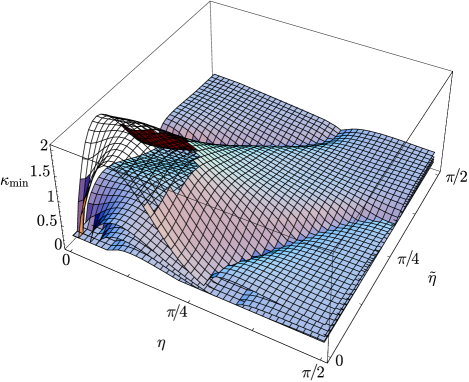
FIG. 5.: Here the quality of the adiabatic approximation $\delta g^{(2)}_{\rm ad}$ [Eq. (14)] in describing the Aharonov-Bohm oscillations is shown. We used Eq. (27) and set $\gamma^{C}=\gamma^{D}=0.1$. The surfaces shown are, from top to bottom, the minimal value of $\kappa_{\rm min}$ required for an agreement $\Delta<0.01$, $0.05$, $0.1$, and $0.2$ [Eq. (27)]. As expected, for $\eta=\tilde{\eta}=0$ we have $\delta g^{(2)}=\delta g^{(2)}_{\rm ad}$. For tilt angles $\eta,\,\tilde{\eta}\approx\pi/2$, the agreement is obtained at low $\kappa_{\rm min}$, whereas at $\eta=\tilde{\eta}\approx 0.25$ larger fields are necessary.

We now discuss the effects of different parameters on $\kappa$ and on the minimal magnetic fields required to reach adiabaticity, thus indicating favorable experimental setups. If we consider rings of increasing circumference $L$, we can see from Eq. (7) that the minimal magnetic field strength needed decreases as $B_{\rm ad}\propto L^{-2}$. However, to observe the Berry phase, dephasing must not be too strong, so the condition $L\lesssim 2L_{C/D}$ should still be met. We note that for two equal fields, the first term of $\gamma^{C}\propto L_{C}^{-2}$ in Eq. (8) depends on $L^{2}$, which restrains us from taking $L>2L_{\varphi}$, whereas the second one depends for $B=B_{\rm ad}$ on $L^{-2}$. So not only the high magnetic fields needed for adiabaticity, but also the small arm widths $a$ required to minimize strong dephasing due to the penetrating flux, disfavors experimental setups with very small $L$.

Introducing more impurities and thus decreasing the diffusion coefficient $D$ leads to slower motion of the electrons around the ring, giving their spins more time to adjust to the local magnetic texture. Thus, the field strengths required for adiabaticity to occur decrease as $B_{\rm ad}\propto D$, which can be seen from Eq. (7). However, such slow diffusion also leads to shorter dephasing lengths $L_{T},\,L_{\varphi}\propto D^{1/2}$; assuming that $\tau_{\varphi}$ remains constant. To avoid such an additional dephasing, i.e. leaving $\gamma^{C/D}$ unaffected, the sample size must also be decreased as $L\propto D^{1/2}$. Thus, because of $\kappa\propto D^{-1}L^{2}$, no net decrease of the required fields for adiabaticity can be gained by decreasing the diffusion coefficient.

IV Exact calculations with Spin-Orbit Interaction in Diffusive Limit

We turn now to the discussion of Berry phases induced by spin-orbit interaction. Instead of considering an inhomogeneous field, we use here an effective (non-hermitian) Hamiltonian

$$h^{C/D}_{{\scriptscriptstyle\mathit{S}O}} = \frac{L}{(2\pi)^{2}}\frac{\partial^{2}}{\partial x^{2}}+i\kappa\sigma_{1z}-i\tilde{\kappa}\sigma_{2z}$$ (30)

$$+i\frac{\alpha}{\hbar^{2}}\frac{L^{2}}{D(2\pi)^{2}}({\mathbf{e}}_{z}\times\mbox{\boldmath{$\sigma$}}^{(*)})\cdot{\mathbf{p}},$$

with spin-orbit interaction, using a coupling constant $\alpha$ as defined in Ref. [26], and with a Zeeman term from an external magnetic field, which is perpendicular to the ring plane. One arrives at this Hamiltonian by starting from the Feynman path integral representation of the transition amplitude with spin-orbit coupling, as it is given in Ref. [27]. One can then formally decouple orbital and spin motion, and following the steps given in App. A of Ref. [6], one arrives at the effective Schrödinger equation for the cooperon propagator with the Hamiltonian $h^{C}_{\scriptscriptstyle\mathit{S}O}$. The equation with $h^{D}_{\scriptscriptstyle\mathit{S}O}$ for the diffuson, which will be required in Sec. IV B, can be obtained by applying the techniques explained in App. A.

Note that in Eq. (30) the momentum operator is still in the Cartesian coordinate system. Now we adopt a polar coordinate system, with $(x^{\prime},\,y^{\prime})=(r\,\cos{\textstyle\frac{2\pi x}{L}},\,r\,\sin{\textstyle\frac{2\pi x}{L}})$ and $(\partial_{x^{\prime}},\,\partial_{y^{\prime}})=(-\frac{1}{2}\{\sin{\textstyle\frac{2\pi x}{L}},\,\partial_{x}\},\>\frac{1}{2}\{\cos{\textstyle\frac{2\pi x}{L}},\,\partial_{x}\})$, where $x$ denotes the position along the ring and runs from $0$ to $L$. The curly braces denote the anticommutator, which ensures the hermiticity of the momentum operator. We now have

$$h_{\scriptscriptstyle\mathit{S}O}^{C/D} = \frac{L^{2}}{(2\pi)^{2}}\frac{\partial^{2}}{\partial x^{2}}+i\kappa\sigma_{1z}-i\tilde{\kappa}\sigma_{2z}$$ (33)

$$+\frac{\alpha}{\hbar}\frac{L^{2}}{D(2\pi)^{2}}\left.\frac{1}{2}\right\{\sigma_{1x}\cos{\textstyle\frac{2\pi x}{L}}+\sigma_{1y}\sin{\textstyle\frac{2\pi x}{L}}$$

$$\quad\left.-\sigma_{2x}\cos{\textstyle\frac{2\pi x}{L}}\mp\sigma_{2y}\sin{\textstyle\frac{2\pi x}{L}},\>\frac{\partial}{\partial x}\right\}.$$

To diagonalize the Hamiltonian, we follow the ideas used above and use the operators defined in Eq. (9), but now with $f=\tilde{f}=1$:

$$J^{C/D}:=\frac{L}{2\pi i}\frac{\partial}{\partial x}+\frac{1}{2}\sigma_{1z}\pm\frac{1}{2}\sigma_{2z},$$ (34)

which commute with the Hamiltonians $h_{\scriptscriptstyle\mathit{S}O}^{C/D}$, as can be seen using $\left[\{n(x),\,\partial_{x}\},\,\partial_{x}\right]=-\{n^{\prime}(x),\,\partial_{x}\}$. We can now calculate the matrix elements of $h_{\scriptscriptstyle\mathit{S}O}^{C/D}$ in the basis defined in Eq. (10), with $f=\tilde{f}=1$, as

$$\left\langle j,\alpha\beta\left|h_{\scriptscriptstyle\mathit{S}O}^{C}\right|j^{\prime},\alpha^{\prime}\beta^{\prime}\right\rangle=\delta_{jj^{\prime}}\left(\begin{array}[]{*{3}{c@{\:}}c}-(j-1)^{2}+i\kappa\!-\!i\tilde{\kappa}\hfil\>&iS\left(j-{\textstyle\frac{1}{2}}\right)\hfil\>&iS\left(-j+{\textstyle\frac{1}{2}}\right)\hfil\>&\>\>\>\>\>0\\ iS\left(j-{\textstyle\frac{1}{2}}\right)\hfil\>&-j^{2}+i\kappa+i\tilde{\kappa}\hfil\>&\>\>\>\>\>0\hfil\>&iS\left(-j-{\textstyle\frac{1}{2}}\right)\\ iS\left(-j+{\textstyle\frac{1}{2}}\right)\hfil\>&\>\>\>\>\>0\hfil\>&-j^{2}-i\kappa-i\tilde{\kappa}\hfil\>&iS\left(j+{\textstyle\frac{1}{2}}\right)\\ \>\>\>\>\>0\hfil\>&iS\left(-j-{\textstyle\frac{1}{2}}\right)\hfil\>&iS\left(j+{\textstyle\frac{1}{2}}\right)\hfil\>&-(j+1)^{2}-i\kappa\!+\!i\tilde{\kappa}\end{array}\right),$$ (35)

and

$$\left\langle j,\alpha\beta\left|h_{\scriptscriptstyle\mathit{S}O}^{D}\right|j^{\prime},\alpha^{\prime}\beta^{\prime}\right\rangle=\delta_{jj^{\prime}}\left(\begin{array}[]{*{3}{c@{\:}}c}-j^{2}+i\kappa\!-\!i\tilde{\kappa}\hfil\>&iS\left(j-{\textstyle\frac{1}{2}}\right)\hfil\>&iS\left(-j-{\textstyle\frac{1}{2}}\right)\hfil\>&\>\>\>\>\>0\\ iS\left(j-{\textstyle\frac{1}{2}}\right)\hfil\>&-(j\!-\!1)^{2}+i\kappa\!+\!i\tilde{\kappa}\hfil\>&\>\>\>\>\>0\hfil\>&iS\left(-j+{\textstyle\frac{1}{2}}\right)\\ iS\left(-j-{\textstyle\frac{1}{2}}\right)\hfil\>&\>\>\>\>\>0\hfil\>&-(j\!+\!1)^{2}-i\kappa\!-\!i\tilde{\kappa}\hfil\>&iS\left(j+{\textstyle\frac{1}{2}}\right)\\ \>\>\>\>\>0\hfil\>&iS\left(-j+{\textstyle\frac{1}{2}}\right)\hfil\>&iS\left(j+{\textstyle\frac{1}{2}}\right)\hfil\>&-j^{2}-i\kappa\!+\!i\tilde{\kappa}\end{array}\right).$$ (36)

In Eqs. (35) and (36), we have introduced a dimensionless spin-orbit coupling parameter

$$S=\frac{\alpha}{\hbar D}\frac{L}{2\pi}.$$ (37)

By comparing Eqs. (7) and (37), we note that while $\kappa$ is quadratic in $L$, the parameter $S$ is only linearly dependent on $L$. If we define an effective field angle for diffusive motion with spin-orbit coupling

$$\tan{\eta_{{\scriptscriptstyle\mathit{S}O}}}=S/\kappa,$$ (38)

and anticipate the Berry phase to be of the form $\Phi^{g}=\cos{\eta}$, we obtain for $S\gg\kappa$ the dependency $\Phi^{g}\approx\kappa/S\propto L$. Thus the phase can now be enhanced by increasing the size of the ring. However, the phase cannot be increased arbitrarily; for large $L$, the assumption $S\gg\kappa$ becomes invalid.

A Magnetoconductance

We shall now calculate the magnetoconductance with the formula from Ref. [6]

$$\delta g_{\scriptscriptstyle\mathit{S}O}=-\frac{e^{2}}{\pi\hbar}\frac{L}{(2\pi)^{2}}\sum_{\alpha,\beta=\pm 1}\left\langle x,\,\alpha,\,\beta\left|\frac{1}{\gamma-h^{C}_{{\scriptscriptstyle\mathit{S}O}}}\right|x,\,\beta,\,\alpha\right\rangle.$$ (39)

With Eq. (35), we obtain the magnetoconductance

$$\delta g_{\scriptscriptstyle\mathit{S}O} = -\frac{e^{2}}{\pi\hbar}\sum_{j=-\infty}^{\infty}{\frac{2\left[4\kappa^{2}+\left(m^{2}+\gamma\right)^{2}\right]\left(m^{2}+\gamma+1\right)+S^{2}\left[8m^{4}+2m^{2}\left(4\gamma-1\right)+2\gamma+1\right]}{\left[4\kappa^{2}+\left(m^{2}+\gamma\right)^{2}\right]\left[m^{4}+2m^{2}\left(\gamma-1\right)+\left(\gamma+1\right)^{2}\right]+S^{2}\left(m^{2}+\gamma\right)\left[4m^{4}+m^{2}\left(4\gamma-3\right)+\gamma+1\right]}},$$ (40)

where $m=j-2\phi/\phi_{0}$ contains the Aharonov-Bohm flux. In Sec. V we will see that in the “adiabatic” limit $\kappa,\,S\gg 1$ the magnetoconductance $\delta g_{\scriptscriptstyle\mathit{S}O}$ will show some similar properties as for inhomogeneous fields, in particular a peak-splitting in the power spectrum, see Fig. 11.

B Conductance Fluctuations

We turn now to a discussion of the recent experiment by Morpurgo et al.[12] by specifying the parameters of the effective Hamiltonian $h^{C/D}_{\scriptscriptstyle\mathit{S}O}$, as given in Eqs. (30), (35), and (36). In Ref. [12], conductance measurements were performed on an InAs ring, with nearly ballistic transport. For the parameters given, [12] $\alpha=5.5\times 10^{-10}\>{\rm eV\,cm}$, $L=6.6\>\mu{\rm m}$, ${v_{\rm F}}=9.8\times 10^{7}\>{\rm cm}/{\rm s}$, $\ell=1.0\>\mu{\rm m}$, and $D={v_{\rm F}}\ell/2=4.9\times 10^{3}\>{\rm cm}^{2}/{\rm s}$, we calculate with Eq. (37) a numerical value of $S\approx 1/50$. Compared to this, the strength of the Zeeman term $\kappa\approx 1/2$ (with $|g|=15$) is much larger. Within the diffusive approximation, this spin-orbit coupling $S\ll\kappa$ gives only a negligible contribution to the effective Hamiltonian $h^{C/D}$ [Eq. (30)] and thus does not produce any Berry phase effects. This very same finding has also been obtained in Ref. [28], based on a slightly different reasoning. Still, we show in Sec. V that a spin-splitting produced by spin-orbit interaction can be obtained in the “adiabatic regime” $\kappa,\,S\gg 1$, which, however, is in the opposite limit to the one reported in Ref. [12]. So although we cannot give a quantitative explanation of the experiment[12] here, we can offer a qualitative interpretation, see Fig. 13. Further, there is an uncertainty in the spin-orbit coupling parameter $\alpha$ in InAs, as it was recently pointed out[29], and more experiments might be needed to clarify this issue.

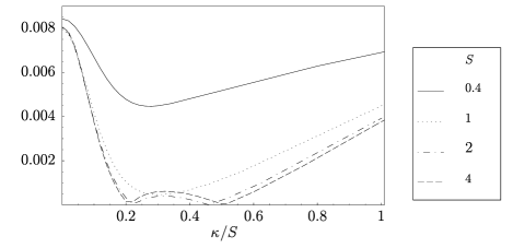
FIG. 6.: The normalized amplitudes of the $h/2e$ oscillations of the UCFs with spin-orbit coupling, $\delta g^{(2)}_{\scriptscriptstyle\mathit{S}O}$. The power spectrum of the Aharonov-Bohm oscillations was calculated at different values $\kappa=\tilde{\kappa}$ of the perpendicular fields by varying the Aharonov-Bohm flux $0\leq\phi=\tilde{\phi}\leq 1$. From the power spectrum, the frequency contribution of the $h/2e$ oscillation was normalized by the zero frequency contribution and is shown here as a function of $\kappa/S$. We have assumed $T=0$ and $\gamma^{C}=\gamma^{D}=0.1$.

To this end we calculate the exact, i.e. without assuming any form of adiabaticity, expression for the conductance fluctuations $\delta g_{\scriptscriptstyle\mathit{S}O}^{(2)}$ in the presence of spin-orbit interaction. With the block-diagonalization of the Hamiltonian $h^{C/D}_{\scriptscriptstyle\mathit{S}O}$ [Eqs. (35), (36)] we obtain the propagators required in the formula for the conductance correlator [Eq. (4)]. We use Mathematica to obtain an explicit algebraic expression for $\delta g^{(2)}_{\scriptscriptstyle\mathit{S}O}$ (which is lengthy and thus not reproduced here) and plot it in Fig. 6 (see also Figs. 12 and 13). From this plot we deduce that in a configuration with spin-orbit coupling, the Aharonov-Bohm oscillations vanish for certain values of $S$ and $\kappa$. It is remarkable that this happens, for $S\geq 2$, at the fixed ratios $\kappa/S=0.2$ and $0.5$, which can be ascribed again to some effective magic angles. Thus we see that Berry phase-like effects occur in $\delta g^{(2)}_{\scriptscriptstyle\mathit{S}O}$ as the amplitudes of the Aharonov-Bohm oscillations become dependent on $\kappa/S$. This resembles the case for inhomogeneous fields, where the amplitudes of the Aharonov-Bohm oscillations became dependent on the tilt angle $\eta$ of the magnetic field due to the Berry phase, as it was shown in Sec. III A.

V Peak Splittings in Power Spectra

A Frequency Shifts in $\delta g$ and $\delta g^{(2)}$

We discuss now the emergence of the Berry phase in terms of a splitting of the frequencies of the Aharonov-Bohm oscillations in the magnetoconductance[6, 9] $\delta g$ and in the UCFs[6] $\delta g^{(2)}$, which can be made visible in the power spectrum.[12] Both quantities depend on the spin-dependent total phase $\Phi_{\alpha}$, given here for the special case of the texture defined in Eq. (1) and for two equal fields ${\mathbf{B}}={\mathbf{\tilde{}}{B}}$,

$$\Phi_{\pm 1} = 2\phi/\phi_{0}\pm\cos{\eta}=2\phi/\phi_{0}\pm\frac{1}{\sqrt{1+(B_{\parallel}/B_{z})^{2}}}$$ (41)

$$\approx 2\phi/\phi_{0}\pm B_{z}/B_{\parallel}=B_{z}\left(2B_{\phi_{0}}^{-1}\pm B_{\parallel}^{-1}\right).$$ (42)

The approximation used here is valid for small perpendicular fields $B_{z}\ll B_{\parallel}$. We have introduced $B_{\phi_{0}}=\phi_{0}/A$ as the perpendicular field which produces a flux of one flux quantum $\phi_{0}$ through the ring, i.e. the period of an Aharonov-Bohm oscillation in $\phi$. The Berry phase is not sensitive to the area enclosed by the ring; thus we prefer here to describe oscillations in $B_{z}$ rather than in $\phi$. As both $\delta g$ and $\delta g^{(2)}$ contain periodic terms in $\Phi_{1}$ and $\Phi_{-1}$, they exhibit oscillations in $B_{z}$ with the Aharonov-Bohm frequency for homogeneous fields, $2B_{\phi_{0}}^{-1}$, shifted (at $B_{z}=0$) by the frequency

$$\frac{1}{\Delta B_{1}}=\pm\frac{1}{B_{\parallel}}\,,$$ (43)

which results in a peak splitting in the power spectrum.

These splittings are, however, generally on the order of the resolution of the spectrum, which makes it difficult to make them visible. If the perpendicular field is varied from $-B_{\rm max}$ to $B_{\rm max}$, the discrete Fourier transform (DFT) of such an interval has a resolution of $1/2B_{\rm max}$, i.e. the sampling frequencies are separated by this value. Thus, the peak-splitting term can only be made visible if this resolution is high enough, i.e. $1/2B_{\rm max}\leq 1/B_{\parallel}$, or

$$B_{\rm max}\geq\frac{1}{2}B_{\parallel}.$$ (44)

We note that this restriction is still consistent with the approximation made in Eq. (41), since for $B_{z}=B_{\parallel}/2$ the approximated value of the Berry phase is larger than the exact value by only a factor of $\sqrt{5}/2\approx 1.1$.

Now we consider the case beyond the above approximation. Here, an estimate for the frequency shifts can be obtained by counting the additional oscillations upon increasing $B_{z}$. In this estimation we again neglect the change in frequency of the Aharonov-Bohm oscillations while $B_{z}$ is increased. However, now we take the mean value of the frequency instead of the frequency at $B_{z}=0$ as in Eq. (43). Varying $B_{z}$ from $0$ to $B_{\rm max}$ changes the Berry phase contribution to $\Phi_{\pm 1}$ [Eq. (41)] from $0$ to $\pm\cos{\eta|_{B_{z}=B_{\rm max}}}$, and so we obtain the mean frequency shift

$$\frac{1}{\Delta B_{2}} = \pm\frac{1}{\sqrt{B_{\rm max}^{2}+B_{\parallel}^{2}}}\approx\pm\frac{1}{B_{\parallel}}\left(1-\frac{B_{\rm max}^{2}}{2B_{\parallel}^{2}}\right).$$ (45)

When we have calculated the DFT of $\delta g$ and $\delta g^{(2)}$, we have confirmed the predictions given above, i.e. we do not observe a peak splitting in the $2B_{\phi_{0}}^{-1}$ frequency for low $B_{\rm max}$, due to an insufficient resolution of the DFT. However, we do see a peak splitting in the DFT for higher fields (see Figs. 8, 9), which vanishes again for $B_{\rm max}\gg B_{\parallel}$. Since studies of the DFT suffer from a restricted resolution, it might be more promising to search for the Berry phase via the effects discussed in Sec. III A.

Finally, we point out that an anisotropic $g$ factor affects the size of the frequency splitting. If the $g$ factor perpendicular to the ring, $g_{z}$, is larger than the one in the plane of the ring, $g_{\parallel}$, the Berry phase dependence on $B_{z}$ increases while the Aharonov-Bohm phase remains unaffected. As the total phase is $\Phi_{\pm 1}\approx 2\phi/\phi_{0}\pm g_{z}B_{z}/g_{\parallel}B_{\parallel}$, the frequency splitting is increased by a factor of $g_{z}/g_{\parallel}$.

B Frequency shifts in $\delta g^{(2)}_{\rm hom}$ for homogeneous fields

At this point it is important to realize that frequency shifts can also appear in the conductance fluctuations $\delta g^{(2)}$ for homogeneous fields, i.e. even when there is no Berry phase present. For homogeneous fields the evaluation of Eq. (4) is straightforward, as $h^{C/D}$ [Eq. (12)] becomes diagonal, see also App. C. We evaluate the DOS terms, i.e. the terms containing ${\rm Re}\,{\rm Tr}\,\hat{\chi}_{\omega}\hat{\chi}_{\omega}$ in Eq. (4), in the low temperature limit for $\eta=\tilde{\eta}=0$:

$$\delta g^{(2)}_{DOS,\atop C/D}\propto{\rm Re}\!\!\sum_{j\atop\alpha,\tilde{\alpha}=\pm 1}\frac{1}{\left[\gamma+(j\!-\!\Phi^{\scriptscriptstyle C/D})^{2}+i(\alpha\kappa\!+\!\tilde{\alpha}\tilde{\kappa})\right]^{2}}$$ (46)

$$\!\!\approx\frac{2\pi}{\gamma^{3/2}}+\!\sum_{\alpha,\tilde{\alpha}}\sum_{n=1}^{\infty}\!\frac{2\pi^{2}n}{\gamma}e^{-2\pi n\sqrt{\gamma}}\cos{\!\left[\!2\pi n\!\left(\!\Phi^{\scriptscriptstyle C/D}\!\!+\!\frac{\alpha\kappa\!+\!\tilde{\alpha}\tilde{\kappa}}{2\sqrt{\gamma}}\right)\!\right]},$$ (47)

where we have defined $\Phi^{C/D}=\phi/\phi_{0}\pm\tilde{\phi}/\phi_{0}$. The approximation on the second line of Eq. (46) is valid for $\gamma\gg 1/4\pi^{2},\>\alpha\kappa+\tilde{\alpha}\tilde{\kappa}$. From Eq. (46), we see that the Zeeman term itself already leads to a frequency splitting. So, for instance, if we take the Fourier transform of $\delta g^{(2)}(B_{z},\,-B_{z})$ with respect to $B_{z}$, we can observe a frequency splitting of the $h/e$ oscillations of the diffuson contribution in the DOS term $\delta g^{(2)}_{DOS,\,D}$, given by

$$\frac{1}{\Delta B_{\mathit{Z}eeman}}=\pm\frac{g{\mu_{\rm B}}}{4\hbar D}\frac{L_{D}L}{2\pi}.$$ (48)

We checked numerically that the estimated frequency splitting [Eq. (48)] is correct within 20 percent even for parameters beyond the assumptions made for the second line of Eq. (46). It is important to keep this property of the conductance fluctuations $\delta g^{(2)}$ in mind, when searching for Berry phase effects. If vanishing Aharonov-Bohm oscillations or peak splittings in the power spectrum are used to identify the presence of a Berry phase, one has to rule out effects coming from the Zeeman term in the UCFs, e.g. by comparison with the results for homogeneous fields.

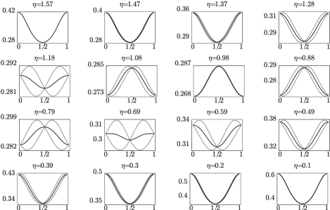
FIG. 7.: The magnetoconductance $\delta g$ in units of $-2e^{2}/h$ as a function of the Aharonov-Bohm flux $2\phi/\phi_{0}$, for different tilt angles $\eta$ of the external field. We have chosen the dephasing $\gamma=0.1$ and the field $B_{\parallel}$ parallel to the ring plane to be constant, defined through $B_{\parallel}\propto\kappa_{\parallel}=\kappa\,\sin{\eta}=2.0$. The magnetoconductance is shown in black, while its contribution from the different spins $\alpha=\pm 1$ are scaled by a factor of two and drawn in gray.

C Numerical Evaluations

We shall now numerically evaluate the magnetoconductance $\delta g$ for a ring in an inhomogeneous field. We base our analysis on the calculations from Ref. [11]. In Fig. 7 we show the Aharonov-Bohm oscillations for different tilt angles $\eta$ of the external field ${\mathbf{B}}$, which is set so strong that we are well within the adiabatic regime. We can readily see that for $\eta\approx\pi/3$ a phase shift of $\pi$ occurs, which comes directly from the Berry phase, compared to the oscillations at $\eta=0$ and $\eta=\pi/2$. For the intermediate tilt angles the effect of the Berry phase is only visible in the amplitude of the Aharonov-Bohm oscillations, as the phase shifts for the two spin directions occur with opposite signs and thus—if both spin directions contribute equally—no phase-shift effect is visible.

As such a phase shift at $\pi/3$ might not be easy to observe, studying signs in the power spectrum provides an interesting alternative,[12] even though it requires a sufficiently high resolution, as discussed in Sec. V A. Indeed, we can observe a peak splitting in the spectrum of the magnetoconductance, as shown in the inset of Fig. 8. We notice an even more distinct feature: the Aharonov-Bohm oscillations vanish at two magic tilt angles, $\cos{\eta}=0.4,\,0.75$, of the field. The mechanism for this effect is exhibited in Fig. 7, where it is shown how the two contributions of the different spins suppress the oscillations.

FIG. 8.: The Aharonov-Bohm oscillations in the magnetoconductance $\delta g$ as a function of the perpendicular field $B_{z}$, shown here as $\kappa_{z}=\kappa\,\cos{\eta}$. The radial field component has a magnitude of $B_{\parallel}\propto\kappa_{\parallel}=\kappa\,\sin{\eta}=2.0$ and $\gamma=0.1$. The vanishing oscillations near $\kappa_{z}\approx 0.9,\,2.3$ (for the magic angle $\cos{\eta}\approx 0.4,\,0.75$) are striking; this a direct consequence of the Berry phase, arising from a canceling of the oscillating contributions of opposite spin directions. The inset shows the power spectrum[30] where a peak splitting is visible.

At this point, we would like to stress that the peak splitting depends strongly on the different dephasing terms. In particular, one cannot rely on calculations where the dephasing due to the inhomogeneous fields is not properly taken into account. So if the dephasing $\gamma$ due to homogeneous effects is very small, e.g. on the order of $1/100$, the amplitude of the oscillations gets reduced drastically as soon as the tilt angle $\eta$ changes from $\pi/2$ to a smaller, nonzero value, since the field inhomogenity causes additional dephasing. Thus the Fourier transform of such oscillations has a dominant contribution only from the first few oscillations close to $\pi/2$. This suppression of the remaining oscillations acts as a narrowing of the data window[31] and leads to a widening of the peaks in the power spectrum, masking the peak splitting. The oscillations are further suppressed by the additional dephasing arising from an increasing perpendicular field, which penetrates the ring arms. Of course, it is possible to remove this unwanted over-emphasizing of certain oscillations from experimental data in a post-processing step; using a standard windowing function (we used the Hann window[31] for the inset of Fig. 8) for DFTs greatly reduces this problem, in addition to the usual reduction of components leakage of neighboring frequencies in the power spectrum.[31]

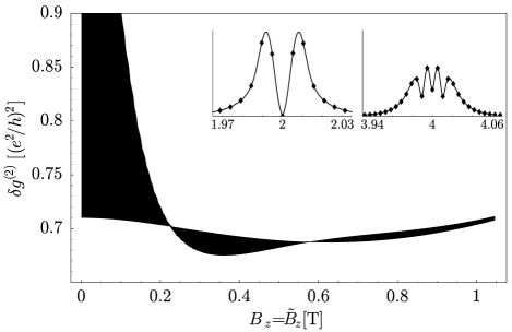
FIG. 9.: The UCFs $\delta g^{(2)}$ for ${\mathbf{B}}={\mathbf{\tilde{}}{B}}$ plotted as function of $B_{z}$ (see first part of Sec. III A). While the printing resolution is not high enough to show the Aharonov-Bohm oscillations, the envelope clearly illustrates the non-monotonic behavior of their amplitudes, which vanish at the magic angles $\eta=0.72,1.15$. We have taken a fixed radial component for both fields of $B_{\parallel}=\tilde{B}_{\parallel}=0.5\>{\rm T}$. We have assumed $L=3\>\mu{\rm m}$, $D=65\>{\rm cm}^{2}/{\rm s}$, and $T=0$. The dephasing was taken into account according to Eq. (8), with the parameters $L_{\varphi}=1.5\>\mu{\rm m}$, and $a=60\>{\rm nm}$. The two insets show the contributions of the $h/2e$ and $h/4e$ oscillations to the power spectrum[30] in arbitrary units plotted against the frequency in units of $\phi_{0}^{-1}$. The right inset was scaled by a factor of 10. For the particular range of $B_{z}$ chosen here, there is a peak splitting visible for the $h/2e$ oscillations, while we observe four peaks around the $h/4e$ frequency.

For the conductance fluctuations $\delta g^{(2)}$, we will further illustrate the effects of the two configurations discussed in Section III A. In Fig. 9 we show the Aharonov-Bohm oscillations occurring in $\delta g^{(2)}$ when the fields are equal, i.e. ${\mathbf{B}}={\mathbf{\tilde{}}{B}}$. Taking the discrete Fourier transform of $\delta g^{(2)}$ over the range $B_{z}=0,\dots,1\>{\rm T}$, yields a clear peak splitting of the contribution of the $h/2e$ oscillations to the power spectrum, see left inset in Fig. 9. We notice a splitting into four peaks of the contribution of the $h/4e$ oscillations (right inset of Fig. 9). They only occur in the exact solution $\delta g^{(2)}$, whereas $\delta g^{(2)}_{\rm ad}$ exhibits only two peaks if we ignore the $\eta$, $\tilde{\eta}$-dependent dephasing, i.e. set $\tilde{\gamma}^{C/D}_{\eta,\,\tilde{\eta}}\to\gamma^{C/D}$ and $P\to 0$ in Eq. (14). We point out that the frequency shifts for the $n$th harmonics of the Aharonov-Bohm oscillations increase with $n$ and are thus are better resolved in the power spectrum with increasing $n$.

We plot $\delta g^{(2)}({\mathbf{\tilde{}}{B}})$ in Fig. 10 for the special case ${\mathbf{\tilde{}}{B}}=(0,\,0,\,\tilde{B}_{z})$ homogeneous (see also Sec. III A).

Finally, we consider the power spectrum of the magnetoconductance $\delta g_{\scriptscriptstyle\mathit{S}O}$ in the presence of spin-orbit coupling. We use Eq. (40) and ignore for simplicity dephasing due to the external magnetic fields penetrating the arms of the ring. Indeed, taking the Fourier transform of the magnetoconductance, a spin splitting can be observed. However, the splitting is not as pronounced as in the case for inhomogeneous fields. Especially important, the splitting is only visible for sufficiently large dephasing parameters $\gamma$ (produced by inelastic scattering), which can be seen in Fig. 11. In contrast to the effects discussed before, using a windowing function was not sufficient to identify a peak splitting for moderately small dephasing parameters $\gamma\lesssim 0.3$. Qualitatively, however, the power spectra of the magnetoconductance for inhomogeneous magnetic fields and for spin-orbit coupling agree, with both showing a peak splitting.

FIG. 10.: The UCFs $\delta g^{(2)}$ for a homogeneous texture of ${\mathbf{B}}$ plotted as function of $\tilde{B}_{z}$ (see second part of Sec. III A). We have taken the homogeneous field as $B_{z}=0.5\>{\rm T}$, and $B_{\parallel}=0\>{\rm G}$ and have fixed the radial component for the other field as $\tilde{B}_{\parallel}=0.43\>{\rm T}$. The remaining parameters are chosen as in Fig. 9. The inset shows the power spectrum[30] in arbitrary units plotted against the frequency in units of $\phi_{0}^{-1}$, which exhibits a splitting in the $h/e$ contributions.

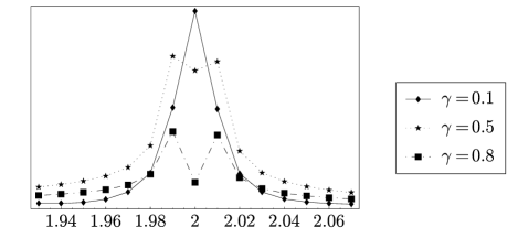
FIG. 11.: The power spectrum of the magnetoconductance $\delta g_{\scriptscriptstyle\mathit{S}O}(B)$ with spin-orbit coupling, Eq. (40), in arbitrary units plotted against the frequency in units of $\phi_{0}^{-1}$. We have chosen $S=4$ and taken the Fourier transform of the magnetoconductance for $0\leq\kappa\leq 4$. We show the power spectrum for three different values of the dephasing parameter $\gamma$, where we have downscaled the values for $\gamma=0.1$ by a factor of $10$. Note that a peak splitting occurs only for the cases with larger dephasing.

The UCFs with spin-obit interaction $\delta g^{(2)}_{\scriptscriptstyle\mathit{S}O}$ are plotted in Fig. 12 as a function of the perpendicular fields $B_{z}=\tilde{B}_{z}$. We observe a Berry phase-like frequency splitting in the power spectrum. However, as this splitting is rather small, it is only visible in the $h/4e$ oscillations, where the splitting is twice as large as in the $h/2e$ oscillations. Again, the suppression of the Aharonov-Bohm oscillations at $\kappa/S\approx 0.25$ is a distinct feature of a Berry phase-like effect.

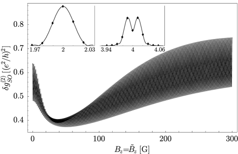
FIG. 12.: The UCFs $\delta g^{(2)}_{\scriptscriptstyle\mathit{S}O}$ with spin-orbit interaction for ${\mathbf{B}}={\mathbf{\tilde{}}{B}}$ plotted as function of $B_{z}$. We have taken $\alpha=1.0\times 10^{-9}\>{\rm eV\,cm}$, $L=12.5\>\mu{\rm m}$, $D=2.0\times 10^{-2}\>{\rm m}^{2}/{\rm s}$, $g=15$, and have assumed $T=0$. This gives us $S=1.6$ [Eq. (37)], and $\kappa(B_{z}=300\>{\rm G})=4.2$ [Eq. (7)]. The dephasing was taken into account according to Eq. (8), with the parameters $L_{\varphi}=5.0\>\mu{\rm m}$, and $a=120\>{\rm nm}$. The envelope of the Aharonov-Bohm oscillations shows a non-monotonic behavior, which also appears in the UCFs for inhomogeneous fields $\delta g^{(2)}$ (see Fig. 9). The $h/2e$ oscillations are strongly suppressed at $B_{z}\approx 30\>{\rm G}$, which corresponds to $\kappa/S\approx 0.25$, as can also be seen from Fig. 6. However, this suppression is not very obvious in this figure, since $h/4e$ oscillations are present for $B_{z}\approx 30\>{\rm G}$. The two insets show the contributions of the $h/2e$ and $h/4e$ oscillations to the power spectrum in arbitrary units[30] plotted against the frequency in units of $\phi_{0}^{-1}$. The right inset was scaled by a factor of 10. For the particular range of $B_{z}$ chosen here, there is only a single peak visible for the $h/2e$ oscillations, while we observe a small peak splitting around the $h/4e$ frequency.

A quantity, which was subject of recent studies,[12, 28] is the disorder-averaged squared power spectrum of the conductance

$$\Big{\langle}\big{|}g(\nu)\big{|}^{2}\Big{\rangle}=\big{|}\big{\langle}g(\nu)\big{\rangle}\big{|}^{2}+\Big{\langle}\big{|}g(\nu)-\langle g(\nu)\rangle\big{|}^{2}\Big{\rangle}.$$ (49)

On the one hand, we recognize that the first term contains the Fourier transform of the (averaged) magnetoconductance $\delta g$, which has frequency contributions from its $h/2e$ oscillations. On the other hand, the second term of Eq. (49) is given through the conductance fluctuations $\delta g^{(2)}$ as $\int\int dB_{z}d\tilde{B}_{z}\exp{\{2\pi i\nu(B_{z}-\tilde{B}_{z})\}}\delta g^{(2)}({\mathbf{B}},{\mathbf{\tilde{}}{B}})$. This term contributes frequencies corresponding to $h/e$ oscillations, coming from the diffuson term $\delta g^{(2)}_{D}$ in the conductance fluctuations. Thus, if we now investigate $h/e$ oscillations, we can restrict our studies to the second term of Eq. (49). We have evaluated $\langle|g(\nu)|^{2}\rangle$ for inhomogeneous fields, with the parameters given in the caption of Fig. 9. A splitting of the frequency corresponding to the $h/e$ oscillations was observed and was identified not to result from the Berry phase but from the Zeeman term already present in the case of homogeneous fields [Eq. (48)]. Then we examined $\langle|g_{\scriptscriptstyle\mathit{S}O}(\nu)|^{2}\rangle$ with spin-orbit coupling for various parameters. An additional peak splitting to the one produced by the Zeeman term [Eq. (48)] appears for some specific parameters, i.e. for $S$ large enough to reach “adiabaticity” and for large enough sampling intervals of $B_{z}$, $\tilde{B}_{z}$ to obtain a sufficiently high resolution in the power spectrum. In Fig. 13 we see such a splitting of the $h/e$ contribution into four peaks. However, using the parameters given in Ref. [12], we have $S\approx 1/50$ and $\kappa\approx 1/2$ (see Sec. IV B) and in this regime we do not observe any peak splitting, in accordance with Ref. [28].

FIG. 13.: The disorder-averaged squared power spectrum of the conductance $\langle|g_{\scriptscriptstyle\mathit{S}O}(\nu)|^{2}\rangle$ [Eq. (49)] with spin-orbit interaction plotted as function of $\nu$ in units of $\phi_{0}^{-1}$, normalized by the zero frequency contribution. We have taken the same parameters as in Fig. 12, but now with $\alpha=2.0\times 10^{-9}\>{\rm eV\,cm}$, and thus $S=3.2$ [Eq. (37)]. We have calculated the second term of Eq. (49) explicitly (see text), while taking $B_{z},\,\tilde{B}_{z}\in[-B_{\rm max},\,B_{\rm max}]$ with $B_{\rm max}=0.1\>{\rm T}$, which gives us a maximal value $\kappa_{\rm max}=14$ [Eq. (7)]. The peak splitting into the inner two peaks is produced by the spin-orbit interaction, while the larger satellite peaks result from the Zeeman term [Eqs. (46) and (48)].

VI Conclusion

We have calculated the exact conductance fluctuations $\delta g^{(2)}$ for a special texture [Eq. (1)] and given its adiabatic approximation $\delta g^{(2)}_{\rm ad}$. In addition to the already known differential equations for the cooperon we have derived the ones for the diffuson in inhomogeneous magnetic fields (App. A). With the result $\delta g^{(2)}_{\rm ad}$ the dephasing due to inhomogeneous fields became explicit and could be compared with previous calculations[6] where adiabatic eigenstates were used and this dephasing was only implemented with a phenomenological parameter. Then we have described some magic tilt angles of the magnetic field at which the Berry phase suppresses the Aharonov-Bohm oscillations. We have used this effect to illustrate how the adiabatic criterion becomes gradually satisfied. We have calculated numerically the required magnetic field strength for which the adiabatic approximation becomes valid and have shown that the adiabatic criterion is less stringent for diffusive than for ballistic motion, thus confirming previous findings.[6, 11]

Furthermore, we have calculated the magnetoconductance and the conductance fluctuations for a diffusive conductor in the presence of spin-orbit coupling. A numerical analysis revealed a non-monotonic behavior of the amplitudes of the Aharonov-Bohm oscillations and peak-splittings in the power spectrum—observations that are similar to the Berry phase effects we have found for inhomogeneous magnetic fields.

Finally, we have described the mechanisms which lead to peak splittings in the power spectrum of magnetoconductance and UCFs and have discussed numerical requirements to make such peaks splittings visible.

A Differential equations for Cooperon and Diffuson

Here we will transform the exact conductance correlator for diffusive systems and arbitrary magnetic textures to make a Schrödinger equation approach [5] possible. Further we will derive the explicit differential equation for the diffuson propagator (the one for the cooperon has been derived previously [6]).

The conductance correlator has been derived in Ref. [6], using diagrammatic techniques, and is given by

$$\delta g^{(2)} = \left(\frac{2e^{2}D}{hL^{2}}\right)^{2}\int d\epsilon\,d\epsilon^{\prime}n^{\prime}(\epsilon)\,n^{\prime}(\epsilon^{\prime})\int d{\mathbf{x}}\,d{\mathbf{x}}^{\prime}\sum_{\alpha_{1},\alpha_{2},\alpha_{3},\alpha_{4}}\left\{\frac{1}{d}\left|\chi^{C}_{\alpha_{1}\alpha_{2},\alpha_{3}\alpha_{4}}({\mathbf{x}},{\mathbf{x}^{\prime}},\omega)\right|^{2}\right.$$ (A1)

$$+ \left.2\,{\rm Re}\left[\chi^{C}_{\alpha_{1}\alpha_{2},\alpha_{3}\alpha_{4}}({\mathbf{x}},{\mathbf{x}^{\prime}},\omega)\chi^{C}_{\alpha_{2}\alpha_{1},\alpha_{4}\alpha_{3}}({\mathbf{x}^{\prime}},{\mathbf{x}},\omega)\right]+\left[\chi^{C}\rightarrow\chi^{D}\right]\right\},$$ (A2)

where $n^{\prime}(\epsilon)$ is the derivative of the Fermi function, $\hbar\omega=\epsilon-\epsilon^{\prime}$, and $d$ describes the dimension of the system with respect to the mean free path $l$. The inverse Fourier transform of the cooperon/diffuson propagators $\chi^{C/D}({\mathbf{x}^{\prime}},{\mathbf{x}},w)$ were obtained [6, 27] as

$$\chi^{C/D}_{\alpha_{1}\alpha_{2},\alpha_{3}\alpha_{4}}({\mathbf{x}^{\prime}},{\mathbf{x}};t^{\prime},t) = \theta(t^{\prime}-t)\int_{{\mathbf{R}}(t)={\mathbf{x}}}^{{\mathbf{R}}(t^{\prime})={\mathbf{x}^{\prime}}}{\cal D}{\mathbf{R}}\exp\left\{-\frac{1}{4D}\int_{t}^{t^{\prime}}d\tau|{\mathbf{\dot{}}{R}}|^{2}\right\}$$ (A3)

$$\times \exp\left\{i\frac{e}{\hbar}\int_{t}^{t^{\prime}}d\tau\>\left[{\mathbf{\dot{}}{R}}\cdot{\mathbf{A}}^{\rm em}({\mathbf{R}}(\tau))+{\mathbf{\dot{}}{R}}^{\pm}\cdot{\mathbf{\tilde{}}{A}}^{\rm em}({\mathbf{R}}^{\pm}(\tau))\right]\right\}$$ (A4)

$$\times \left\langle\alpha_{4}\alpha_{2}\left|{\cal T}\exp\left\{i\frac{g{\mu_{\rm B}}}{2\hbar}\int_{t}^{t^{\prime}}d\tau\left[{\mathbf{B}}({\mathbf{R}}(\tau))\cdot\mbox{\boldmath{$\sigma$}}_{1}-{\mathbf{\tilde{}}{B}}({\mathbf{R}}^{\pm}(\tau))\cdot\mbox{\boldmath{$\sigma$}}_{2}\right]\right\}\right|\alpha_{3}\alpha_{1}\right\rangle,$$ (A5)

where ${\mathbf{R}}^{-}(\tau)={\mathbf{R}}(t^{\prime}+t-\tau)$ is the time-reversed path of ${\mathbf{R}}^{+}\equiv{\mathbf{R}}$.

For explicit evaluation it is convenient to transform this path-integral representation into a differential equation. In the case of the diffuson we first have to eliminate the time-reversed paths. As a result of reverting the time integration, an additional sign appears in the second term of the electromagnetic vector potential. For the Zeeman interaction we can use the relation

$$\left\langle\alpha_{2}\left|{\cal T}\exp\left\{-i\frac{g{\mu_{\rm B}}}{2\hbar}\int_{t}^{t^{\prime}}d\tau\,{\mathbf{\tilde{}}{B}}({\mathbf{R}}^{-}(\tau))\mbox{\boldmath{$\sigma$}}\right\}\right|\alpha_{1}\right\rangle=\left\langle\alpha_{1}\left|{\cal T}\exp\left\{i\frac{g{\mu_{\rm B}}}{2\hbar}\int_{t}^{t^{\prime}}d\tau\,{\mathbf{\tilde{}}{B}}({\mathbf{R}}(\tau))\mbox{\boldmath{$\sigma$}}\right\}\right|\alpha_{2}\right\rangle^{*}$$ (A6)

$$\qquad\qquad=\left\langle\alpha_{1}\left|{\cal T}\exp\left\{-i\frac{g{\mu_{\rm B}}}{2\hbar}\int_{t}^{t^{\prime}}d\tau{\mathbf{\tilde{}}{B}}({\mathbf{R}}(\tau))\mbox{\boldmath{$\sigma$}}^{*}\right\}\right|\alpha_{2}\right\rangle.$$ (A7)

The latter equation can be proven by writing the time-ordered product as a Dyson series and by inserting a resolution of unity in spin space between all products $({\mathbf{B}}(x_{j})\mbox{\boldmath{$\sigma$}})({\mathbf{B}}(x_{j+1})\mbox{\boldmath{$\sigma$}})$, thereby arriving at an expression with terms of the form $\left\langle\alpha\left|B_{i}(x_{j})\sigma_{i}\right|\beta\right\rangle^{*}$. Such terms are the complex conjugate of Pauli matrix elements multiplied by the real number $B_{i}(x_{j})$. So we can rewrite them as $\left\langle\alpha\left|B_{i}(x_{j})\sigma_{i}^{*}\right|\beta\right\rangle$, remove the previously inserted unities, and go back to the time-ordered product.

Now we can give the differential equations for the propagators

$$\Bigglb(\frac{\partial}{\partial t^{\prime}}+D\left[-i\frac{\partial}{\partial{\mathbf{x}^{\prime}}}-\frac{e}{\hbar}\left[{\mathbf{A}}^{\rm em}({\mathbf{x}^{\prime}})\pm{\mathbf{\tilde{}}{A}}^{\rm em}({\mathbf{x}^{\prime}})\right]\right]^{2}$$ (A8)

$$\qquad\qquad-i\frac{g{\mu_{\rm B}}}{2\hbar}\left[{\mathbf{B}}({\mathbf{x}^{\prime}})\cdot\mbox{\boldmath{$\sigma$}}_{1}-{\mathbf{\tilde{}}{B}}({\mathbf{x}^{\prime}})\cdot\mbox{\boldmath{$\sigma$}}_{2}^{(*)}\right]\Biggrb)\hat{\chi}^{C/D}({\mathbf{x}^{\prime}},{\mathbf{x}};t^{\prime},t)=\delta({\mathbf{x}^{\prime}}-{\mathbf{x}})\delta(t^{\prime}-t)\hat{1\!\!1},$$ (A9)

where $\hat{\chi}^{C/D}({\mathbf{x}^{\prime}},{\mathbf{x}};t^{\prime},t)$ is a matrix in four-dimensional spin space. The upper sign is for the cooperon [6], the lower sign and the complex conjugate of $\mbox{\boldmath{$\sigma$}}_{2}$ for the diffuson. Passing to Fourier space and operator notation, the above equation becomes

$$\left(i\omega-D\frac{(2\pi)^{2}}{L^{2}}h^{C/D}\right)\hat{\chi}^{C/D}_{\omega}=\hat{1\!\!1},$$ (A10)

where the effective Hamiltonian $h^{C/D}$ is defined in Eq. (6).

Finally we express the conductance correlation in terms of the operators $\chi^{C/D}_{\omega}$. We note that with $\chi^{C}_{\alpha_{1}\alpha_{2},\alpha_{3}\alpha_{4}}({\mathbf{x}},{\mathbf{x}^{\prime}},\omega)^{*}=\langle{\mathbf{x}^{\prime}},\alpha_{4}\alpha_{2}|\hat{\chi}^{C}_{\omega}|{\mathbf{x}},\alpha_{3}\alpha_{1}\rangle^{*}=\langle{\mathbf{x}},\alpha_{3}\alpha_{1}|\hat{\chi}^{C\dagger}_{\omega}|{\mathbf{x}^{\prime}},\alpha_{4}\alpha_{2}\rangle$ , and $\chi^{D}_{\alpha_{1}\alpha_{2},\alpha_{3}\alpha_{4}}({\mathbf{x}},{\mathbf{x}^{\prime}},\omega)^{*}=\langle{\mathbf{x}^{\prime}},\alpha_{4}\alpha_{1}|\hat{\chi}^{D}_{\omega}|{\mathbf{x}},\alpha_{3}\alpha_{2}\rangle^{*}=\langle{\mathbf{x}},\alpha_{3}\alpha_{2}|\hat{\chi}^{D\dagger}_{\omega}|{\mathbf{x}^{\prime}},\alpha_{4}\alpha_{1}\rangle$ we can simplify the terms in Eq. (A1):

$$\int d{\mathbf{x}}\,d{\mathbf{x}^{\prime}}\sum_{\alpha_{1},\ldots,\alpha_{4}}\left|\chi^{C/D}_{\alpha_{1}\alpha_{2},\alpha_{3}\alpha_{4}}({\mathbf{x}},{\mathbf{x}^{\prime}},\omega)\right|^{2}={\rm Tr}\,\hat{\chi}^{C/D}_{\omega}\hat{\chi}^{C/D\dagger}_{\omega},$$ (A11)

and

$$\int d{\mathbf{x}}\,d{\mathbf{x}^{\prime}}\sum_{\alpha_{1},\ldots,\alpha_{4}}\chi^{C/D}_{\alpha_{1}\alpha_{2},\alpha_{3}\alpha_{4}}({\mathbf{x}},{\mathbf{x}^{\prime}},\omega)\chi^{C/D}_{\alpha_{2}\alpha_{1},\alpha_{4}\alpha_{3}}({\mathbf{x}^{\prime}},{\mathbf{x}},\omega)={\rm Tr}\,\hat{\chi}^{C/D}_{\omega}\hat{\chi}^{C/D}_{\omega}.$$ (A12)

B Finite Temperature Integrals

We shall explain here the integrations performed to obtain Eq. (26). We are interested in

$$I=\int d\epsilon^{\prime}n^{\prime}(\epsilon^{\prime})J=\int d\epsilon^{\prime}n^{\prime}(\epsilon^{\prime})\int d\epsilon\,n^{\prime}(\epsilon)\left(\frac{1}{d}\frac{1}{(\epsilon-\epsilon^{\prime}+a)^{2}+c^{2}}+2{\rm Re}\frac{1}{(i\epsilon-i\epsilon^{\prime}+ia-c)^{2}}\right)$$ (B1)

with $a,c$ real and $c>0$. We consider a rectangular integration contour $\Gamma$ with one side lying on the real axis, extending $M=2\pi l/\beta$ towards the positive imaginary axis and the same amount on each side of the real axis. For any positive integer $l$, the absolute value of the Fermi function is bounded above on such a contour: $|n(z)|\Big{|}_{\Gamma}<2$. The integrands considered further below are a product of the Fermi function and a rational function decaying with at least $|z|^{-2}$. The integral of these products over the section of $\Gamma$ in the upper half plane, will thus vanish for $M\to\infty$, as we have $|z|\geq M$ on this contour. We further note, that the complex expansion of the Fermi function $n(z)$ has its poles at $z=i\omega_{n}$, where $\omega_{n}=\pi n/\beta$ are the Matsubara frequencies and $n$ is an odd integer.

We expand the first rational function in Eq. (B1) into partial fractions and then integrate $J$ by parts:

$$J = \int d\epsilon n(\epsilon)\left\{\frac{1}{d}\frac{1}{2ic}\left(\frac{1}{(\epsilon-\epsilon^{\prime}+a-ic)^{2}}-\frac{1}{(\epsilon-\epsilon^{\prime}+a+ic)^{2}}\right)+2{\rm Re}\frac{-2}{(\epsilon-\epsilon^{\prime}+a+ic)^{3}}\right\}$$ (B2)

$$= {\rm Re}\int d\epsilon n(\epsilon)\left\{\frac{1}{d}\frac{i}{c(\epsilon-\epsilon^{\prime}+a+ic)^{2}}-\frac{4}{(\epsilon-\epsilon^{\prime}+a+ic)^{3}}\right\}.$$ (B3)

We now evaluate the integral along the contour described above. As the poles of the rational functions in Eq. (B3) are in the lower half plane at $\epsilon^{\prime}-a-ic$, they are not within the integration contour. Applying Cauchy’s residue theorem and accounting for the residues of the Fermi function ${\rm res}\,n(z)|_{z=i\omega_{n}}=(-1/\beta)$ yields

$$J=\frac{2\pi}{\beta}{\rm Re}\sum_{n\,\rm{odd}>0}\left\{\frac{1}{d}\frac{1}{c(i\omega_{n}-\epsilon^{\prime}+a+ic)^{2}}+\frac{4i}{(i\omega_{n}-\epsilon^{\prime}+a+ic)^{3}}\right\}.$$ (B4)

For the second integration in Eq. (B1), we replace the expression in braces in the above equation by its complex conjugate. As before, we first integrate by parts over $\epsilon^{\prime}$ and apply the residue theorem afterwards. This results in

$$I = \frac{4\pi}{\beta}{\rm Re}\sum_{n\,\rm{odd}>0}\int d\epsilon^{\prime}n(\epsilon^{\prime})\left\{\frac{1}{d}\frac{1}{c(i\omega_{n}+\epsilon^{\prime}-a+ic)^{3}}+\frac{6i}{(i\omega_{n}+\epsilon^{\prime}-a+ic)^{4}}\right\}$$ (B5)

$$= \frac{8\pi^{2}}{\beta^{2}}{\rm Re}\sum_{n,m\,\rm{odd}>0}\left\{\frac{1}{d}\frac{1}{c(\omega_{n}+\omega_{m}+ia+c)^{3}}+\frac{6}{(\omega_{n}+\omega_{m}+ia+c)^{4}}\right\}.$$ (B6)

C UCFs $\delta g^{(2)}_{\rm hom}$ for homogeneous fields

For homogeneous fields we have $\eta=\tilde{\eta}=0$ and $f=0$, thus the hamiltonians $h^{C/D}$ [Eq. (11)] become diagonal with the matrix elements $j^{2}+i\alpha\kappa-i\tilde{\alpha}\tilde{\kappa}$. Now we evaluate the propagators $\hat{\chi}^{C/D}$ [Eq. (5)] and by evaluating the integrals over the Fermi functions in Eq. (4) explicitly by using standard Matsubara techniques, as explained in App. B. We obtain $\delta g^{(2)}_{\rm hom}=\delta g^{(2)}_{{\rm hom},\,C}+\delta g^{(2)}_{{\rm hom},\,D}$, where

$$\delta g^{(2)}_{{\rm hom},\atop C/D} =\left(\frac{e^{2}}{h}\right)^{2}\!\frac{1}{8\pi^{6}}\left(\frac{L^{2}}{L_{T}^{2}}\right)^{2}{\rm Re}\,\sum_{\alpha,\tilde{\alpha}=\pm 1}\sum_{j=-\infty}^{\infty}\left.\sum_{n,m}\right.^{\prime}$$ (C3)

$$\left\{\frac{1}{d\,(\gamma^{C/D}\!+j^{2})\left[b_{nm}+\gamma^{C/D}\!+j^{2}\!+\!i(\alpha\kappa-\tilde{\alpha}\tilde{\kappa})\right]^{3}}\right.$$

$$\quad\left.+\frac{6}{\left[b_{nm}+\gamma^{C/D}\!+j^{2}\!+\!i(\alpha\kappa-\tilde{\alpha}\tilde{\kappa})\right]^{4}}\right\},$$

and we have introduced $b_{nm}=(n+m)(L/L_{T})^{2}/4\pi$. Here $n$ and $m$ are positive, odd integers. The Aharonov-Bohm flux is implemented by replacing $j\to j-(\phi/\phi_{0}\pm\tilde{\phi}/\phi_{0})$. For further evaluation we now set $\kappa=\tilde{\kappa}$. We describe the summation of cooperon and diffuson terms with a prefactor $\beta$, which is $1$ if both terms contribute and $2$ if time-reversal symmetry is broken, so the cooperon contribution vanishes. Thus we have $\delta g^{(2)}_{\rm hom}\approx(2/\beta)\delta g^{(2)}_{{\rm hom},\,D}$ and from now on we only consider the dephasing parameter $\gamma=\gamma^{D}=L^{2}/(2\pi L_{\varphi})^{2}$, according to Eq. (8).

If the spin-channel mixing is suppressed (i.e. $\kappa\gg\gamma$) in Eq. (C3), we can replace the sum over the spins $\sum_{\alpha\tilde{\alpha}}$ by the number of spin states $g_{s}$. For weaker magnetic fields ($\kappa\ll\gamma$) we have full spin degeneracy and obtain the factor $g_{s}^{2}$. Accounting for valley degeneracy yields a factor $g_{v}^{2}$.

Since we will check our results against the ones given in Ref. [24], where one-dimensional systems were considered, we take $d=1$. Since we will evaluate some limiting cases below, where $L\gg 2\pi L_{\varphi}$, we have $\gamma\gg 1$ and can therefore replace the $j$-sum in Eq. (C3) by an integral. The Aharonov-Bohm phase can then be removed by shifting the integration variable $j$ and we obtain

$$\delta g^{(2)}_{\rm hom} = \left(\frac{e^{2}}{h}\right)^{2}\!\frac{1}{8\pi^{6}}\frac{2g_{s}^{2}g_{v}^{2}}{\beta}\left(\frac{L^{2}}{L_{T}^{2}}\right)^{2}\left.\sum_{n,m}\right.^{\prime}\int_{-\infty}^{\infty}dj$$ (C5)

$$\left\{\frac{1}{d\,(\gamma+j^{2})\left[b_{nm}+\gamma+j^{2}\right]^{3}}\right.\left.+\frac{6}{\left[b_{nm}+\gamma+j^{2}\right]^{4}}\right\}.$$

In the limit $(2\pi)^{2}L_{\varphi}^{2}\ll L^{2},2\pi L_{T}^{2}$, we have

$$\frac{2\pi L_{T}^{2}}{L^{2}}\,(\gamma+j^{2})\geq\frac{L_{T}^{2}}{2\pi L_{\varphi}^{2}}\gg 1.$$ (C6)

Thus, we can use Poisson’s summation formula to replace the summation over $n$ and $m$ in Eq. (C5) by integration to arrive at

$$\delta g^{(2)}_{\rm hom} = \frac{3}{4\pi^{4}}\frac{g_{s}^{2}g_{v}^{2}}{\beta}\left(\frac{e^{2}}{h}\right)^{2}\int_{-\infty}^{\infty}\frac{dj}{\left(\gamma+j^{2}\right)^{2}}$$ (C8)

$$=3\,\frac{g_{s}^{2}g_{v}^{2}}{\beta}\left(\frac{e^{2}}{h}\right)^{2}\left(\frac{L_{\varphi}}{L}\right)^{3}.$$

We now consider another limit, $2\pi L_{T}^{2}\ll L^{2},(2\pi)^{2}L_{\varphi}^{2}$. Again, we start from Eq. (C5), but now we first calculate the integral over $j$, which has the dominant contribution $\pi\gamma^{-1/2}b^{-3}$ since $1\ll\gamma\ll b_{nm}$. Thus we obtain

$$\delta g^{(2)}_{\rm hom} = \frac{4}{\pi}\frac{g_{s}^{2}g_{v}^{2}}{\beta}\left(\frac{e^{2}}{h}\right)^{2}\frac{L_{T}^{2}}{L^{2}}\frac{L_{\varphi}}{L}\left.\sum_{n,m}\right.^{\prime}\frac{1}{\left(\frac{1}{2}(n+m)\right)^{3}}$$ (C9)

$$= \frac{2\pi}{3}\frac{g_{s}^{2}g_{v}^{2}}{\beta}\left(\frac{e^{2}}{h}\right)^{2}\frac{L_{T}^{2}}{L^{2}}\frac{L_{\varphi}}{L}.$$ (C10)

Indeed, our results $\delta g^{(2)}_{\rm hom}$ given in Eqs. (C8) and (C9) agrees with these of Ref. [24]. Thus, on the one hand, we have confirmed that the result from Ref. [6] [used in Eq. (4)] is consistent with earlier calculations.[20, 23, 24] On the other hand, in Eq. (C3) we have given an explicit formula (not known before as far as we are aware of) describing how the spin-channel mixing becomes suppressed for increasing magnetic fields, such that $\delta g^{(2)}_{\rm hom}$ contains a prefactor $g_{s}^{2}$ for low and $g_{s}$ for high magnetic fields.

REFERENCES

- [1] M. V. Berry, Proc. R. Soc. London, Ser. A: 392, 45 (1984).
- [2] For a collection of relevant reprinted articles and commentary, see A. Shapere and F. Wilczek, Geometric Phases in Physics (World Scientific, Singapore, 1989).
- [3] D. Loss, P. M. Goldbart and A. V. Balatsky, Phys. Rev. Lett. 65, 1655 (1990).
- [4] D. Loss, P. M. Goldbart and A. V. Balatsky, 1990, in Granular Nanolelectronics, D. K. Ferry, J. R. Barker and C. Jacoboni (eds.), NATO ASI Series B: Physics 251 (Plenum, New York, 1991).
- [5] D. Loss and P.M. Goldbart, Phys. Rev. B 45, 13544 (1992).
- [6] D. Loss, H. Schoeller, and P.M. Goldbart, Phys. Rev. B 48, 15218 (1993).
- [7] Y. Lyanda-Geller, I.L. Aleiner, and P.M. Goldbart Phys. Rev. Lett. 81, 3215 (1998).
- [8] D. Loss and P.M. Goldbart, Phys. Lett. A 215, 197 (1996).
- [9] A. Stern, Phys. Rev. Lett. 68, 1022 (1992)
- [10] S.A. van Langen, H.P.A. Knops, J.C.J. Paasschens, and C.W.J. Beenakker, Phys. Rev. B 59, 2102 (1999).
- [11] D. Loss, H. Schoeller, and P.M. Goldbart, Phys. Rev. B 59, 13328 (1999).
- [12] A. F. Morpurgo, J. P. Heida, T. M. Klapwijk, B. J. van Wees, and G. Borghs, Phys. Rev. Lett. 80, 1050 (1998).
- [13] A.G. Aronov and Y.B. Lyanda-Geller, Phys. Rev. Lett. 70, 343 (1993).
- [14] P.D. Ye, S. Tarucha and D. Weiss, Proceeding of ICPS 24, Israel (1998).
- [15] T.M. Jacobs and N. Giordano, Superlattices and Microstructures 23, 635 (1998).
- [16] P. Mohanty and R.A. Webb, Phys. Rev. Lett. 84, 4481 (2000).
- [17] R. Häussler, PhD thesis, Universität Karlsruhe, 1999.
- [18] G. Nunes, APS Centennial Meeting (1999) QC21,6.
- [19] A.G. Aronov and Yu.V. Sharvin, Rev. Mod. Phys. 59, 755 (1987).
- [20] P.A. Lee, A.D. Stone and H. Fukuyama, Phys. Rev. B 35, 1039 (1987).
- [21] Implementing magnetic textures with different winding numbers and can be easily done by replacing the coefficient of in Eq. (9) with . This will result in different diagonal elements in the matrices given below. As we have verified, within this approach the only further generalization of the magnetic texture is an arbitrary rotation axis of the field.[32] Otherwise it is not possible to find a linear combination of and Pauli matrices which commutes with .
- [22] As every quantity is periodic in with period one, we see that has a periodic dependence on the Aharonov-Bohm fluxes , .
- [23] B.L. Al’tshuler and D.E. Khmel’nitskii, Pis’ma Zh. Eksp. Teor. Fiz. 42, 291 (1985) [JETP Lett. 42, 359 (1985)].
- [24] C.W.J. Beenakker and H. van Houten, Phys. Rev. B 37, 6544 (1988).
- [25] P. Mohanty, E.M.Q. Jariwala, and R.A. Webb, Phys. Rev. Lett. 78, 3366 (1997).
- [26] Yu. A. Bychkov, V.I. Mel’nikov and E.I. Rashba, Sov. Phys. JETP 71, 401 (1990) [Zh. Eksp. Teor. Fiz. 98, 717 (1990)].
- [27] S. Chakravarty and A. Schmid, Phys. Rep. 140, 193 (1986).
- [28] A.G. Mal’shukov, V.V. Shlyapin and K.A. Chao, Phys. Rev. B 60, 2161 (1999).
- [29] S. Brosig, K. Ensslin, R.J. Warburton, C. Nguyen, B. Brar, M. Thomas, and H. Kroemer, Phys. Rev. B 60, 13989 (1999).
- [30] The full line in the power spectrum is provided as a guide to the eye. It was obtained by zero-padding the data before calculating the DFT.[31]
- [31] W.H. Press, S.A. Teukolsky, W.T. Vetterling, and B.P. Flannery, Numerical Recipes in C (Cambridge University Press, England, 1993), Chap. 12.
- [32] H.A. Engel, Diploma thesis, Universität Basel, 1999.