Super-radiant light scattering from trapped Bose Einstein condensates

Abstract

We propose a new formulation for atomic side mode dynamics from super-radiant light scattering of trapped atoms. A detailed analysis of the recently observed super-radiant light scattering from trapped bose gases [S. Inouye et al., Science 285, 571 (1999)] is presented. We find that scattered light intensity can exhibit both oscillatory and exponential growth behaviors depending on densities, pump pulse characteristics, temperatures, and geometric shapes of trapped gas samples. The total photon scattering rate as well as the accompanied matter wave amplification depends explicitly on atom number fluctuations in the condensate. Our formulation allows for natural and transparent interpretations of subtle features in the MIT data, and provides numerical simulations in good agreement with all aspects of the experimental observations.

03.75.Fi,42.50.Fx,32.80.-t

I INTRODUCTION

The successful discovery of Bose-Einstein condensation (BEC) in dilute trapped atoms [1] provided significant momentum for research into quantum degenerate gases. In analogy with laser theory, condensation results in a coherent matter wave field, which has since been identified [2], and several important optical analogous effects including four-wave mixing [3], superradiance [4], coherent matter wave growth [5] were demonstrated. Theoretical studies of these phenomenon in degenerate BEC systems [6, 7] pointed out the important role of correlations and competitions among matter wave side modes, i.e. multi-mode nature of even a single component condensate due to center of mass (CM) motional effects. For a harmonically trapped condensate, these multi-modes can be conveniently expressed in terms of quantized motional states with equal energy spacing. Theoretical investigations of light scattering from such trapped atoms are complicated since both the elastic and inelastic spectra can include contributions from many different motional states.

In this article, by proposing a new identification of trapped atomic side modes for light scattering from a plane wave excitation, we attempt for a detailed interpretation of the recently observed off-resonant super-radiant light scattering [4]. This constitutes an example of using light scattering as a spectroscopic tool to probe properties of trapped degenerate quantum gas. Our investigations show that quantum statistics of the condensate can have a drastic effect on the properties of scattered photons [8, 9]. Our formalism takes advantage of the recent success with atomic multi-modes [10] to provide a clean interpretation of all aspects of the experimental observations [4]. Similar approaches can also be used to clarify physical pictures of the more recent BEC Bragg spectroscopy experiments [11, 12].

II formulation

Our model describes light scattering of trapped atoms from excitation due to an intense far off-resonant plane wave pump field. The proto-type system is illustrated in Fig. 1 as arranged in the MIT experiment [4]. The atomic sample is assumed dilute and atoms are of the alkali type with a single valance electron. Two electronic states [$g$ ($e$) for ground (excited)] are connected by a real electronic dipole moment $d$. In units of $\hbar=1$ and in length gauge, our model Hamiltonian takes the form

$$H = \sum_{\sigma=g,e}\int d\vec{r}\,\Psi^{{\dagger}}_{\sigma}(\vec{r})H_{A\sigma}\Psi_{\sigma}(\vec{r})+\int d\vec{k}\omega_{k}b_{\vec{k}}^{{\dagger}}b_{\vec{k}}$$ (1)

$$+ \frac{1}{2}{\Omega_{0}(t)}\int d\vec{r}\,\Psi_{e}^{{\dagger}}(\vec{r})e^{i\vec{k}_{0}\cdot\vec{r}}\Psi_{g}(\vec{r})+h.c.$$ (2)

$$+ \int d\vec{r}\int d\vec{k}\,g(\vec{k})\Psi_{e}^{{\dagger}}(\vec{r})e^{i\vec{k}\cdot\vec{r}}b_{\vec{k}}\Psi_{g}(\vec{r})+h.c.,$$ (3)

under dipole and rotating wave approximation. $H_{A\sigma}=-\nabla^{2}/2M+V_{\sigma}(R)+E_{\sigma}$ is the atomic Hamiltonian consists of CM kinetic energy (atomic mass $M$), trapping potential $V_{\sigma}$, and electronic excitation energies in the rotating frame $E_{g}=0,E_{e}=\Delta=\omega_{A}-\omega_{0}$. $\Delta$ is large since the pump field at frequency $\omega_{0}$ is far detuned from the atomic transition frequency $\omega_{A}$. The dipole interaction between an atom and the pump field is described by a time dependent Rabi frequency $\Omega_{0}(t)=\Omega_{0}{\cal T}(\gamma_{0}t)$, with $\Omega_{0}$ the peak value and $\gamma_{0}$ the temporal width of the envelope function ${\cal T}(\gamma_{0}t)$. Both $\Omega_{0}$ and ${\cal T}(\gamma_{0}t)$ are chosen to be real. The polarization and wave vector of the pump pulse are denoted by $\vec{\epsilon}_{0}$ and $\vec{k}_{0}$, respectively. The second term of Eq. (3) describes free electromagnetic fields needed to consider inelastic photon scattering. Their polarization index is suppressed in the wave vector $\vec{k}$. The degenerate atomic fields are described by annihilation (creation) operators $\Psi(\vec{r})$ [$\Psi^{{\dagger}}(\vec{r})$] satisfying appropriate commutators for bosonic or classical Maxwell Boltzman statistics. The operator $b_{\vec{k}}$ $(b^{{\dagger}}_{\vec{k}})$ annihilates (creates) a photon with wave vector $\vec{k}$, polarization $\vec{\epsilon}_{\vec{k}}$, and energy $\omega_{k}=ck-\omega_{0}$ (again in the frame rotating with frequency $\omega_{0}$). Within the two state approximation, dipole coupling between scattered field and an atom is given by $g(\vec{k})=-i\sqrt{ckd^{2}/4\pi^{2}}\vec{\epsilon}_{0}^{\ast}\cdot\vec{\epsilon}_{\vec{k}}$, a slowly varying function of $k$. When the detuning $\Delta$ is much larger than any other frequency scale in the system, the excited state can be eliminated to obtain an effective field theory within the ground atomic motional state manifold [6],

$$H = \int d\vec{r}\,\Psi_{g}^{{\dagger}}(\vec{r})\left[H_{Ag}+\frac{|\Omega_{0}(t)|^{2}}{2\Delta}\right]\Psi_{g}(\vec{r})+\int d\vec{k}\,\omega_{k}b_{\vec{k}}^{{\dagger}}b_{\vec{k}}$$ (4)

$$+ \int d\vec{r}\int d\vec{k}\,g(\vec{k},t)\Psi_{g}^{{\dagger}}(\vec{r})e^{i(\vec{k}-\vec{k}_{0})\cdot\vec{r}}b_{\vec{k}}\Psi_{g}(\vec{r})+h.c.\ .$$ (5)

The AC stark shift term from all field modes except the pump will be neglected in this study since we are interested in regimes when the scattered field intensity remains small. The effective coupling constant $g(\vec{k},t)=\Omega_{0}{\cal T}(\gamma_{0}t)g(\vec{k})/2\Delta$ is now time dependent, and it describes the scattering event in the ground motional state manifold, i.e. the combined effect of absorbing a pump photon to the excited state manifold followed by a spontaneous emission back to the ground state again. In most cases $g(\vec{k},t)$ is a slowly varying function of time. To simplify our discussion we consider a temporal square shaped pulse and thus drop the constant term ${|\Omega_{0}(t)|^{2}}/{2\Delta}$. In contrast to strongly correlated many body systems the trapped atoms are assumed non-interacting, allowing for detailed investigations of their interaction with light fields. The ground state atomic field operator can be expanded in terms of trapped single atom wave function $\phi_{n}$ according to $\Psi_{g}(\vec{r})=\sum_{n}c_{n}\phi_{n}(\vec{r})$. For a harmonic trapping potential, $\phi_{n}(\vec{r})$ is simply the number basis states in position representation with $n=(n_{x},n_{y},n_{z})$ a triplet index. Atomic annihilation and creation operators $c_{n}$ and $c_{n}^{{\dagger}}$ obey bosonic algebra $[c_{n},c_{m}^{\dagger}]=\delta_{nm}$ and $[c_{n},c_{m}]=0$. We then reduce the Hamiltonian (5) to

$$H = H_{0}+H_{R}+H_{AS}+H_{S},$$ (6)

$$H_{0} = \sum_{n}E_{n}c_{n}^{{\dagger}}c_{n}+\int d\vec{k}\,\omega_{k}b_{\vec{k}}^{{\dagger}}b_{\vec{k}},$$ (7)

$$H_{R} = \sum_{n}\int d\vec{k}\,g^{*}(\vec{k},t)\eta_{n,n}(\vec{k}-\vec{k_{0}})c^{{\dagger}}_{n}b_{\vec{k}}^{{\dagger}}c_{n}+h.c.,$$ (8)

$$H_{AS} = \sum_{n}\sum_{m\in(E_{m}>E_{n})}\int d\vec{k}\,g^{*}(\vec{k},t)\eta_{n,m}(\vec{k}-\vec{k_{0}})c^{{\dagger}}_{n}b_{\vec{k}}^{{\dagger}}c_{m}+h.c.,$$ (9)

$$H_{S} = \sum_{n}\sum_{m\in(E_{m}<E_{n})}\int d\vec{k}\,g^{*}(\vec{k},t)\eta_{n,m}(\vec{k}-\vec{k_{0}})c^{{\dagger}}_{n}b_{\vec{k}}^{{\dagger}}c_{m}+h.c.\ .$$ (10)

Figure 2 is a pictorial display of characteristic absorption and emission cycles for Rayleigh, Raman Stokes and anti-Stokes processes. The atomic energy is $E_{n}=E_{0}+\omega_{n}$, consisting of contributions from electronic ground state energy $E_{0}=0$ and CM motion energy $\omega_{n}=\vec{\omega_{t}}\cdot\vec{n}$ with frequency $\vec{\omega_{t}}=(\omega_{x},\omega_{y},\omega_{z})$ for a three dimensional trap. The factor $\eta_{n,m}(\vec{K})=\langle n|\exp{(-i\vec{K}\cdot\vec{r})}|m\rangle$ represents CM motional state dipole transition moment, and is analogous to the Franck-Condon factor in a di-atomic molecular transition. It is simply the matrix element of displacement operator $D(\vec{r})=\exp{(-i\vec{K}\cdot\vec{r})}$ in the number basis and depends on the total recoil momentum $\vec{K}=\vec{k}_{0}-\vec{k}$ from the scattering cycle involving absorption of a pump photon followed by an emission. Within the ground motional states, it acts like a diffraction matrix since it shifts atomic fields around in momentum space. To examine various competing dynamical processes in light scattering described by Eq. (6) we separate the coupling term depending on the energies of the two coupled (initial and final) motional states. This leads to three types of scattering (as in Fig. 2): 1) the elastic Rayleigh scattering described by $H_{R}$ corresponds to events within the same atomic motional states; 2) the Stokes $H_{S}$ and 3) the anti-Stokes $H_{AS}$ Raman scattering into higher (lower) energy motional states. We emphasise that Stokes and anti-Stokes terms here corresponds to the same final electronic state but with increased or decreased energy final motional states. We may thus also call them as “inelastic” Rayleigh scattering.

Before a detailed discussion of the three type scattering events, it is possible to get a crude picture of how each individual interaction term contributes to the dynamics at low temperatures and within a short time scale. When the gas sample is at sufficient low temperatures only low lying atomic motional states are densely occupied and therefore their atomic fields can be approximated as classical variables, while upper motional states are sparsely populated and need to be treated quantum mechanically. Within a short duration, an approximation involving undepleted populations in lower motional states, similar to the parametric pump approximation in nonlinear optical multi-mode coupling, can be made. We can then consider a single motional state (m) and a single resonant scattering field mode with $\vec{k}=\vec{k}_{1}(|\vec{k}_{1}|=k_{0})$, and assume all $N_{0}$ atoms were initially condensed in state $n=(0,0,0)$. We then approximate $c_{0}\sim c_{0}^{\dagger}\sim\sqrt{N_{0}}$, and Hamiltonian (6) is simplified to

$$H = H_{0}+H_{R}+H_{AS}+H_{S},$$ (11)

$$H_{0} = E_{m}c_{m}^{{\dagger}}c_{m}+\omega_{1}b_{\vec{k}_{1}}^{\dagger}b_{\vec{k}_{1}},$$ (12)

$$H_{R} = g^{*}(\vec{k}_{1},t)\eta_{0,0}(\vec{k}_{1}-\vec{k_{0}})N_{0}b_{\vec{k}_{1}}^{{\dagger}}+O(c_{m}^{\dagger}c_{m}b_{\vec{k}_{1}})+h.c.,$$ (13)

$$H_{AS} = g^{*}(\vec{k}_{1},t)\eta_{0,m}(\vec{k}_{1}-\vec{k_{0}})\sqrt{N_{0}}b_{\vec{k}_{1}}^{{\dagger}}c_{m}+h.c.,$$ (14)

$$H_{S} = g^{*}(\vec{k}_{1},t)\eta_{m,0}(\vec{k}_{1}-\vec{k_{0}})\sqrt{N_{0}}c^{{\dagger}}_{m}b_{\vec{k}_{1}}^{{\dagger}}+h.c.\ .$$ (15)

With this simplified model, $H_{R}$ becomes a displacement operation for scattered field mode ($\vec{k}_{1}$); it describes the generation of coherent photon fields in this mode. For the general case of a thermally populated motional state distribution, the total coherent photon fields are distributed accordingly. Terms of order $O(c_{m}^{\dagger}c_{m}b_{\vec{k}_{1}})$ are neglected since the second order quantum processes described by $H_{S}$ and $H_{AS}$ are more important within the short time period discussed here. We see that $H_{AS}$ resembles an atom-polariton Hamiltonian, describing the generation of atom-photon bound states; while $H_{S}$ takes the form of a non-degenerate parametric amplifier Hamiltonian, describing processes of gain, squeezing, and atom-photon entanglement. It should be noted, however, even when both terms $H_{S}$ and $H_{AS}$ are in existence, they can still be grouped as a more general polariton Hamiltonian. Thus, internal fields, i.e. scattered photons inside the atomic sample can always be viewed as being part of an atom-polariton system [13]. Overall photon scattering and emissions from such a system is complicated as internal fields couple to external fields to cause radiative decays of atom-photon polaritons. Their periodic energy exchange implied by $H_{AS}$ could exhibit Rabi type oscillations in the radiated fields. If on the other hand when the motional state $m$ is initially unpopulated, oscillatory behaviors will not appear since $H_{AS}$ can not contribute during the early stages of dynamic interaction.

In the following two sections, we will focus on situations when $H_{S}$ is the dominant interaction term. We start by outlining the required system conditions to achieve this. First we observe that $H_{R}$ governs mostly small angle scattering while both Raman type interactions give rise to mostly large angle scattering. Mathematically this is due to the fact that diagonal elements of the Franck-Condon factors are sharply peaked around axis defined by pump wave vector $\vec{k}_{0}$, while off-diagonal elements favor off-axial scattering for traps of reasonable size $\sim$ a few times the resonant wave length $\lambda_{0}$. The interaction strengths of Rayleigh, Stokes, and anti-Stokes processes all depend on the spatial distribution of atoms, the initial ground state population $N_{0}$, and the laser induced effective dipole interaction strength $g$. In general these different factors compete and complicated pictures of light scattering emerge. But for the current model system, we find that the major role is played by the geometry factor of the system through $\eta_{n,m}$, of which several off-diagonal elements are displayed in Fig. 3.

III SMALL ANGLE SCATTERING AND OSCILLATORY SUPERRADIANCE

Since $H_{R}$ is the leading order interaction term, we will first consider its effect by discussing the process of small angle scattering. In this case, the system dynamics is determined essentially by $H=H_{0}+H_{R}$. Using the property $\eta_{n,n}(\vec{K})=\eta_{n,n}(-\vec{K})$, and taking $g({\vec{k},t})=-i\gamma_{\vec{k}}$ with $\gamma_{\vec{k}}$ real, we obtain the following Heisenberg operator equations of motion

$$\frac{d}{dt}\tilde{c}_{n} = \int d\vec{k}\,\gamma_{\vec{k}}\,\eta_{nn}(\vec{K})P_{\vec{k}}\,\tilde{c}_{n},$$ (16)

$$\frac{d}{dt}P_{\vec{k}} = -i\omega_{k}Q_{\vec{k}},$$ (17)

$$\frac{d}{dt}Q_{\vec{k}} = -i\omega_{k}P_{\vec{k}}-2\gamma_{\vec{k}}F(\vec{K}),$$ (18)

where we have defined auxiliary quadrature operators $P_{\vec{k}}=b_{\vec{k}}-b_{\vec{k}}^{{\dagger}}$, $Q_{\vec{k}}=b_{\vec{k}}+b_{\vec{k}}^{{\dagger}}$, and the form function operator $F(\vec{K})=\sum_{n}\eta_{n,n}(\vec{K})N_{n}$. $\tilde{c}_{n}$ is a slowly variant form of ${c}_{n}$. These equations and the auxiliary operators are similar to those in the theory of collective atomic recoil laser (CARL) [14]. Since $P_{\vec{k}}^{{\dagger}}=-P_{\vec{k}}$, we see that the atom number operator $\tilde{c}_{n}^{\dagger}\tilde{c}_{n}$ is time independent, a testimony of motional state number conservation in Rayleigh scattering. The system of Eq. (18) is integrable and its solutions allow for the calculation of the number of scattered photons

$$\langle b_{\vec{k}}^{+}b_{\vec{k}}\rangle=2\gamma_{\vec{k}}^{2}\left(\frac{\sin{\omega_{k}t/2}}{\omega_{k}}\right)^{2}\left(\left|\sum_{n}\eta_{nn}(\vec{K})N_{n}\right|^{2}+\sum_{n}\left|\eta_{nn}(\vec{K})\right|^{2}\sigma^{2}(N_{n})\right).$$ (19)

We note that the amplitude of scattering light intensity depends on atomic number fluctuations, the variance $\sigma^{2}(N_{n})=\langle N_{n}^{2}\rangle-\langle N_{n}\rangle^{2}$. Depending on the gas temperatures, this fluctuating part could dominate over the first coherent part at larger scattering angles. At very low temperatures, assuming a macroscopic condensed atomic population in the lowest motional state $n=(0,0,0)$, we find

$$\langle b_{\vec{k}}^{{\dagger}}b_{\vec{k}}\rangle=2\gamma_{\vec{k}}^{2}\left(\frac{\sin{\omega_{k}t/2}}{\omega_{k}}\right)^{2}\eta_{0,0}(\vec{K})^{2}[N_{0}^{2}+\xi(N_{0}+\epsilon N_{0}^{2})],$$ (20)

where $\xi=0$ is for a classical gas, and $\epsilon=0$ ($1$) stands for a coherent (Fock) state of the Bose-Einstein condensate with an average of $N_{0}$ atoms. The prefactor in the above two equations involves $\sin(\omega_{k}t)$, a term from the time dependent spectra of the square pump pulse.

At higher temperatures, it was previously calculated that [9],

$$\sum_{n}\eta_{n,n}(\vec{K})N_{n} \approx Ne^{-\frac{1}{2}K_{x}^{2}a_{x}^{2}/\beta\omega_{x}}e^{-\frac{1}{2}K_{y}^{2}a_{y}^{2}/\beta\omega_{y}}e^{-\frac{1}{2}K_{z}^{2}a_{z}^{2}/\beta\omega_{z}},$$ (21)

$$\sum_{n}\left|\eta_{n,n}(\vec{K})\right|^{2}\sigma^{2}(N_{n}) \approx N^{2}\left(\frac{\beta^{3}\omega_{x}\omega_{y}\omega_{z}}{8}\right)e^{-\frac{1}{2}K_{x}^{2}a_{x}^{2}\beta\omega_{x}}e^{-\frac{1}{2}K_{y}^{2}a_{y}^{2}\beta\omega_{y}}e^{-\frac{1}{2}K_{z}^{2}a_{z}^{2}\beta\omega_{z}},$$ (22)

where $\beta=1/k_{B}T$ is proportional to the inverse temperature and the trap ground state size is $a_{\alpha}=\sqrt{(1/2M\omega_{\alpha})}$ in direction $\alpha=x,y,z$. We can readily see that the incoherent part contributes mostly at higher temperatures while the coherent part is more effective at lower temperatures. In order to suppress incoherent large angle scattering we need to satisfy $\frac{1}{2}K_{\alpha}^{2}a_{\alpha}^{2}\beta\omega_{\alpha}\gg 1$, i.e. $E_{\alpha}\beta/2\gg 1$, where $E_{\alpha}=K_{\alpha}^{2}/2M$ is the one dimensional recoil energy. We emphasize that this result is independent of the shape of trapped atomic sample. In terms of recoil temperature $T_{R}=K^{2}/2Mk_{B}$, a sufficient condition is $T\ll 0.5T_{R}$. At such low temperatures coherent Rayleigh scattering dominates. In order to suppress coherent scattering, we can now take advantage of trap size parameters. For a cylindrical sample with $L$ ($W$) the long (short) axis length as in Fig. 1, the coherent scattering is controlled by

$$|\eta_{0,0}(\vec{k}-\vec{k}_{0})|^{2}=e^{-k^{2}L^{2}\sin^{2}{\theta}\cos^{2}{\phi}}e^{-k^{2}W^{2}\sin^{2}{\theta}\sin^{2}{\phi}}e^{-W^{2}(k\cos{\theta}-k_{0})^{2}},$$ (23)

where $z$ axis is chosen to be along the pump field direction and $\theta,\phi$ are polar and azmithual angles of the scattering direction. Typical geometries of current traps are $L=W\sim 10$ ($\mu$m) for spherical traps and $L=10W\sim 200$ ($\mu$m) for cigar shaped traps. Putting these into Eq. (23), we see that the cigar shaped geometry with $L\gg W$ is more effective in suppressing the overall coherent Rayleigh scattering.

Concluding this section we note that under optimal conditions, it is possible to significantly suppress the coherent Rayleigh scattering. Therefore effects of the other wise higher order Raman processes can be made dominant. As reasoned before we can also ignore contributions from anti-Stokes terms at sufficient low temperatures and for short pulse excitation. Thus we shall first develop a simple model considering $H_{S}$ as the only dominant mechanism in describing the directional and exponential superradiance. A more complete treatment including anti-Stokes processes will be considered in Sec. V using a generalized atomic side mode formalism.

IV LARGE ANGLE SCATTERING AND EXPONENTIAL GAIN BEHAVIOR

In this section we consider large angle Raman scattering processes when small angle Rayleigh scattering is suppressed. In the low temperature limit when all atoms are condensed into the ground motional state, we can neglect the ground state atom number fluctuations and approximate $c_{0}=\sqrt{N_{0}}$ as a classical field. The subsequent system dynamics for light scattering can be described by the Hamiltonian

$$H = \sum_{n>0}E_{n}c_{n}^{\dagger}c_{n}+\int d\vec{k}\,\omega_{k}b_{\vec{k}}^{\dagger}{b_{\vec{k}}}$$ (24)

$$+ \sqrt{N_{0}}\int d\vec{k}\left[g^{*}(\vec{k},t)\sum_{n>0}\eta_{n,0}(\vec{k}-\vec{k}_{0})c_{n}^{\dagger}b_{\vec{k}}^{{\dagger}}+h.c.\right].$$ (25)

In this limit, further insight into this problem can be obtained by introducing atomic side mode operators

$$f(\vec{q})=\sum_{n>0}\eta_{0,n}(\vec{q})c_{n}.$$ (26)

Physically these are wave packet operators in the ground state manifold due to absorption of a pump photon followed by emitting a spontaneous photon, resulting in a net momentum transfer of $\vec{q}$. Because momentum conservation is in general violated during photon absorption and emission among two distinct initial and final motional states. These wavepacket operators are the best compromise one can construct to reflect the momentum conservation law for starting in the ground motional state before the absorption and emission cycle. Mathematically, they satisfy the following commutation relation,

$$[f(\vec{q}),f^{{\dagger}}(\vec{p})]=\eta_{00}(\vec{q}-\vec{p})-\eta_{00}(\vec{q})\eta_{00}(-\vec{p})\equiv{\cal D}_{\vec{q}}(\vec{p}).$$ (27)

Of particular interest is the special case of $[f(\vec{q}),f^{\dagger}(\vec{q})]=1-\eta_{00}^{2}(\vec{q})$. These operators can thus be visualized as a deformation on the Weyl-Heisenberg algebra [H(4)] of the original $c_{n}$ operators. On the other hand, if we were to keep $c_{0}$ as an operator, we would need to consider $X_{n0}=c_{n}^{\dagger}c_{0}$ operators [15]. We find that $c_{n}$ can be realized as a bosonic representation of transition operators $X_{n0}$, which obeys a U(3) Lie algebra. A similar deformation on the U(3) could also be proposed. More generally, a class of side mode operators from an arbitrary motional state, not limited to $n=0$ could also be considered as in Sec. V. They represent collective recoil modes corresponding to various transitions from any motional state to higher or lower motional states with a net recoil momentum $\vec{q}$ during the photon absorption and emission cycle.

Neglecting the Doppler effect but keeping the recoil energy term $\omega_{R}(\vec{K})=K^{2}/2M$, we can show that

$$\sum_{n>0}E_{n}\eta_{0,n}(\vec{q})c_{n}\approx[E_{0}+\omega_{R}(\vec{q})]f(\vec{q}).$$ (28)

The equations of motion for the operators are then given by

$$i\frac{d}{dt}f(\vec{q}) = \omega_{R}(\vec{q})f(\vec{q})+\sqrt{N_{0}}\int d\vec{k}\,g^{*}(\vec{k},t)b_{\vec{k}}^{\dagger}\,{\cal D}_{\vec{q}}(\vec{k}_{0}-\vec{k}),$$ (29)

$$i\frac{d}{dt}b_{\vec{k}} = \omega_{k}b_{\vec{k}}+\sqrt{N_{0}}\,g^{*}(\vec{k},t)f^{\dagger}(\vec{k}_{0}-\vec{k}).$$ (30)

We can proceed with standard technique to eliminate the scattered field modes by substituting the formal solution of Eq. (30) into Eq. (29). This yields

$$\frac{d}{dt}f(\vec{q})+i\omega_{R}(\vec{q})f(\vec{q})=F_{L}^{{\dagger}}+N_{0}\int d\vec{k}\,g^{*}(\vec{k},t){\cal D}_{\vec{q}}(\vec{k}_{0}-\vec{k})\int_{0}^{t}d\tau f(\vec{k}_{0}-\vec{k},t-\tau)g(\vec{k},t-\tau)e^{i\omega_{k}\tau},$$ (31)

where the Langevin noise operator $F_{L}(t)$, representing the effect of vacuum fluctuations through the initial scattered field operators $b_{\vec{k}}(0)$, is introduced as in [6]

$$F_{L}(t)=i\sqrt{N_{0}}\int d\vec{k}\,g(\vec{k},t){\cal D}_{\vec{q}}(\vec{k}_{0}-\vec{k})b_{\vec{k}}(0)e^{-i\omega_{k}t}.$$ (32)

This noise term is responsible for triggering the super-radiant emission from the gas sample. It is also needed to satisfy thermal dynamic requirement of fluctuation and dissipation theorem. Since its magnitude is of a lower order in $\sqrt{N_{0}}$, it can be neglected in a semi-classical description of the growth behavior of a small signal gain as in Ref. [6]. In the Markov approximation and with typically small recoils [$\omega_{R}(\vec{q})\rightarrow 0$], we can ignore the slow time dependence of $g(\vec{k},t)$ to obtain

$$\frac{d}{dt}f(\vec{q})=\pi N_{0}\int d\vec{k}\,|g(\vec{k},0)|^{2}{\cal D}_{\vec{q}}(\vec{k}_{0}-\vec{k})f(\vec{k_{0}}-\vec{k})\delta(\omega_{k}).$$ (33)

This expression can be further simplified by noting that $D_{\vec{q}}(\vec{k}_{0}-\vec{k})$ limits the scattering to directions around the end firing modes $\vec{k_{0}}-\vec{q}$ as illustrated in Fig. 1. We then obtain a simple exponential gain behavior for atomic side mode operator according to $f(\vec{q},t)=\exp{(N_{0}G_{\vec{q}}\,t/2)}f(\vec{q},0)$ with the gain parameter given by

$$G_{\vec{q}}=\pi\int d\vec{k}\,|g(\vec{k},0)|^{2}{\cal D}_{\vec{q}}(\vec{k}_{0}-\vec{k})\delta(\omega_{k}).$$ (34)

It is interesting to note that this result is essentially the same as obtained in Ref. [6] except for the difference in ${\cal D}_{\vec{q}}(\vec{p})$. In fact, the condensate shape function was defined in Ref. [6] as $\rho_{\vec{q}}(\vec{k})=\int d\vec{r}\,|\phi_{0}(\vec{r})|^{2}\exp[-i(\vec{k}-\vec{k}_{0}+\vec{q})\cdot\vec{r}]$. It is related our function defined here by ${\cal D}_{\vec{q}}(\vec{k}_{0}-\vec{k})=\rho_{\vec{q}}(\vec{k})-\rho_{\vec{q}}(\vec{k}_{0})\rho_{0}(\vec{k})$.

A more rigorous treatment would include explicitly the role of atomic quantum statistics. Treating $N_{0}$ as an operator, and defining the number operators of recoiled atoms as $n_{\vec{q}}(t)=\left<f^{\dagger}(\vec{q},t)f(\vec{q},t)\right>$, we find $n_{\vec{q}}(t)={\cal G}_{\vec{q}}(t)n_{\vec{q}}(0)$, where the growth function is now defined to be ${\cal G}_{\vec{q}}(t)=\left<\exp{(G_{\vec{q}}tN_{0})}\right>$. In normally ordered form it can be written as

$${\cal G}_{\vec{q}}(t)=\langle e^{tG_{\vec{q}}N_{0}}\rangle=\sum_{j=0}^{\infty}[e^{tG_{\vec{q}}}-1]^{j}\langle c_{0}^{{\dagger}j}c_{0}^{j}\rangle/{j!}.$$ (35)

Clearly, for different quantum statistical distributions, this implies different growth behavior. If we choose the initial condensate to be a coherent state in the motional ground state with an amplitude $\alpha$ such that $\langle c_{0}^{{\dagger}}c_{0}\rangle=|\alpha|^{2}=\langle{N}_{0}\rangle$, we obtain

$${\cal G}_{\vec{q}}(t)=\exp[(e^{G_{\vec{q}}t}-1)\langle{N}_{0}\rangle].$$ (36)

While for a Fock state distribution, the same result as in the semi-classical case applies. We note that at early times ($t\ll 1/G_{\vec{q}}$) both growth curves give identical results irrespective of the atom number statistics of the condensate. At longer times, however, an initial condensate in a coherent state causes side modes to grow faster than an initial Fock state condensate. In Fig. 6, we compare the different growth curves for both cases. Given the same number of condensate atoms, the corresponding super-radiant pulse is then shorter for a coherent state. For the recent MIT experiment [4], it was estimated that with a laser intensity of $10-100$ (mW/cm²), $G_{\vec{q}}\leq 10^{-4}$. Thus for all experimental observed duration, the growth curve is the same irrespective of atom number statistics. We note that if the MIT experiment were operated with a higher pump laser intensity, condensate atom number fluctuations could be probed. In contrast to the small angle Rayleigh scattering where number fluctuations appear as amplitude fluctuations, the large angle Raman scattering studied in this section carries information directly related to condensate number fluctuations.

V SEQUENTIAL SUPERRADIANCE

In the previous section we considered short pulse Stokes Raman scattering in which processes starting from the motional ground state $n=(0,0,0)$ dominate. As a result, the momentum distribution of atoms, sharply peaked around the center-mode $\vec{p}=\vec{0}$ initially, is modified by the appearance of side mode peaks around $\vec{p}=\vec{k}_{0}\pm\vec{k}_{e}$, where $\pm\vec{k}_{e}$ denote the two end firing modes, i.e. emissions along the two ends of an elongated condensate as in Fig. 1. This situation is reminiscent of earlier studies of superfluorescence from an extended and inverted medium [16, 17, 18, 19, 20, 21, 22]. When the Fresnel number of the system, defined as ${\cal F}=\pi(W/2)^{2}/\lambda_{0}L$, is of order unity, a description of the emission can be made in terms of the two end firing modes [16]. For the MIT experiment with $W\sim$ 20 ($\mu$m), $L\sim$ 200 ($\mu$m), and $\lambda_{0}\sim$ 0.6 ($\mu$m), the condition ${\cal F}\sim 1$ is indeed satisfied. With the pump incident along the narrower side of the condensate, possibilities exist for mode couplings into similar end firing modes. This in turn causes recoiling atoms to couple with side modes of $\vec{p}=\vec{k}_{0}\pm\vec{k}_{e}$, and even higher order side modes if the pump stays on for a long period of time. Since $\eta_{0,m}(\vec{k}_{0}\pm\vec{k}_{e})$ is peaked around certain motional state $m_{1}$, this will be reflected in the measured density profile as effective couplings populate state $m_{1}$ from condensate atoms in state $m=(0,0,0)$. With the wave packet formulation, a breadth of ground motional states centered around $m_{1}$ is affected, and it is termed collectively as a side mode to the original condensate. This physical picture is further illustrated by the side mode lattice as given in Fig. 5, where the most important coupling terms from the Hamiltonian Eq. (15) have been selected. We can then truncate the number of nodes involved in the lattice depending on the duration of the pulse to study light scattering dynamics. We introduce generalized side mode operators as follows,

$$f_{n}(\vec{q})=\sum_{m}\eta_{n,m}(\vec{q}-\vec{p})f_{m}(\vec{p}),$$ (37)

with $f_{n}(0)=c_{n}$. Their commutator is evaluated to be

$$[f_{n}(\vec{q}),f_{m}^{{\dagger}}(\vec{p})]=\eta_{n,m}(\vec{q}-\vec{p}).$$ (38)

We can then transform the system Hamiltonian into these side modes to obtain,

$$H = \sum_{n}[E_{n}+\omega_{R}({\vec{q}})]f_{n}^{{\dagger}}(\vec{q})f_{n}(\vec{q})$$ (39)

$$+ \sum_{n,m}\vec{v}_{R}\cdot\vec{P}_{n,m}f_{n}^{{\dagger}}(\vec{q})f_{m}(\vec{q})+\int d\vec{k}\,\omega_{k}b_{\vec{k}}^{{\dagger}}b_{\vec{k}}$$ (40)

$$+ \sum_{n}\int d\vec{k}\,[g^{*}(\vec{k},t)f^{{\dagger}}_{n}(\vec{q}-\vec{k}+\vec{k}_{0})b_{\vec{k}}^{{\dagger}}f_{n}(q)+h.c.].$$ (41)

In the second term, $\vec{v}_{R}=\vec{q}/M$ is the recoil velocity and $\vec{P}_{n,m}$ is the CM momentum matrix elements between the Fock basis $|n\rangle$ and $|m\rangle$. This term couples $f_{n}$ and $f_{n+1}$ and in effect describes the hopping between nearest neighbor motional states. In our discussion below we will neglect this nearest neighbor motional coupling as it is small in the short time scale of the MIT experiment [4, 10]. Keeping only the two end firing photon modes around $\pm\vec{k}_{e}$, we can use Eq. (37) to express side modes around them according to

$$f_{n}(\vec{q}+\vec{k}_{0}-\vec{k})=\sum_{m}\eta_{n,m}(\mp\vec{k}_{e}-\vec{k})f_{m}(\vec{q}+\vec{k}_{0}\pm\vec{k}_{e}).$$ (42)

This implies that by simply examining the dynamics of the two end firing side modes, we can also gain valuable understanding of the behavior of other side modes around them. We further simplify the problem by taking only the diagonal Franck-Condon factors, justified by the reasonably small Fresnel number ${\cal F}$. This allows us to use $f_{n}(\vec{q}+\vec{k}_{0}-\vec{k})\approx\eta_{n,n}(\mp\vec{k}_{e}-\vec{k})f_{n}(\vec{q}+\vec{k}_{0}\pm\vec{k}_{e})$ as $\eta_{n,m}(\mp\vec{k}_{e}-\vec{k})\sim\delta_{nm}$ for modes near the two end firing ones with $\vec{k}\approx\mp\vec{k}_{e}$. Since only $f_{0}(0)$ is initially occupied, this Hamiltonian then couples side modes with $f_{0}(\vec{q})$ for $\vec{q}=0,\vec{k}_{0}\pm\vec{k}_{e},2\vec{k}_{0},2(\vec{k}_{0}\pm\vec{k}_{e})$,$\cdots$ etc. through an infinite hierarchy of equations of nearest neighbor coupling on the triangular lattice as in Fig. 5.

We now discuss effects of the second order side modes. Since the central side mode at $2\vec{k}_{0}$ is coupled to two first order side modes at $\vec{k}_{0}\pm\vec{k}_{e}$, it will grow faster than other second order ones at $2(\vec{k}_{0}\pm\vec{k}_{e})$. Therefore, as indicated in Fig. 5, we close the system of coupled nodes by considering the 4 lattice nodes at $0,\vec{k}_{0}\pm\vec{k}_{e},2\vec{k}_{0}$, which are connected with solid lines. Pulses with longer duration, however, would result in populations grow at higher order lattice nodes. After free expansion on turning off the trapping potential, this particular lattice structure is in fact directly observed in the MIT experiment [4]. The effective Hamiltonian is now given by

$$H =\sum_{\vec{q}}\omega_{R}({\vec{q}})f_{0}^{\dagger}(\vec{q})f_{0}(\vec{q})+\int d\vec{k}\,\omega_{k}b_{\vec{k}}^{{\dagger}}b_{\vec{k}}$$ (44)

$$+\sum_{\vec{q},\epsilon=\pm}[g^{*}(\epsilon\vec{k}_{e},t)B_{\epsilon}^{{\dagger}}f_{0}^{{\dagger}}(\vec{q}-\epsilon\vec{k}_{e}+\vec{k}_{0})f_{0}(\vec{q})+h.c.],$$

where $\vec{q}$ runs over lattice sites $0,\vec{k}_{0}\pm\vec{k}_{e}$ such that we have a truncated problem on the first diamond. The lattice only runs in one direction with a positive $\vec{k}_{0}$ because of the plane wave excitation from one side. The first term of Eq. (44) is due to the recoil shift, and can be eliminated by transforming to an interaction picture. $g(\vec{k},t)$ is a slowly varying function of $\vec{k}$ and is replaced with its value at $\vec{k}=\vec{k}_{e}$ and taken out of the integration over $\vec{k}$. The emission photon wave packet operator is defined as $B_{\epsilon}=\int d\vec{k}\,\eta_{0,0}(\vec{k}-\epsilon\vec{k}_{e})b_{\vec{k}}$ for $\vec{k}$ near $\pm\vec{k}_{e}$. The evolution of its corresponding intensity naturally gives the photon scattering distribution averaged over repeated single-shot experiments. As a collective field operator, $B_{\epsilon}$ takes into account the multi mode but directed (end firing) nature of the scattered field [14]. Although mathematically one obtains

$$[B_{\epsilon},B_{\epsilon^{\prime}}^{\dagger}] =\delta_{\epsilon\epsilon^{\prime}}{\pi^{3/2}\over a_{x}a_{y}a_{z}}.$$ (45)

We take $[B_{\epsilon},B_{\epsilon^{\prime}}^{\dagger}]=\delta_{\epsilon\epsilon^{\prime}}$ since the choice of keeping only end firing modes constrains $\vec{k}$ to be around $\pm\vec{k}_{e}$. Thus one simply has $B_{\epsilon}\sim b_{\epsilon\vec{k}_{e}}$. Other modes around the end firing ones in $B_{\epsilon}$ only contributes to a renormalization of the coupling constant $g$ which we take to be phenomenological. Terms involving $f[2(\vec{k}_{0}\pm\vec{k}_{e})]$ are ignored in this study based on arguments of short pump pulses and low atom number populations.

It is now useful to introduce a more concise notation $a_{0},a_{\pm}$, and $a_{2}$ for $f_{0}(0),f_{0}(\vec{k}_{0}\pm\vec{k}_{e})$, and $f_{0}(2\vec{k}_{0})$. We also treat these operators as commuting with each other as an approximation to Eq. (38) in the limit of large $|\vec{q}-\vec{p}|$. Their Heisenberg operator equations can be derived. It turns out their dynamics is more transparently expressed in terms of the population operators $I_{\pm}=B_{\pm}^{{\dagger}}B_{\pm},N_{\epsilon}=a_{\epsilon}^{{\dagger}}a_{\epsilon}$, and coherence operators $R_{\epsilon\epsilon^{\prime}}=a_{\epsilon}^{{\dagger}}a_{\epsilon^{\prime}}$. We find

$$\frac{d}{dt}I_{\pm} = igR_{0\mp}B_{\pm}+igR_{\pm 2}B_{\pm}+h.c.,$$ (46)

$$\frac{d}{dt}N_{0} = -igR_{0-}B_{+}-igR_{0+}B_{-}+h.c.,$$ (47)

$$\frac{d}{dt}N_{\pm} = igR_{0\pm}B_{\mp}-igR_{\pm 2}B_{\pm}+h.c.,$$ (48)

$$\frac{d}{dt}N_{2} = igR_{+2}B_{+}+igR_{-2}B_{-}+h.c.\ .$$ (49)

In deriving this and other equations to follow, we have consistently used an operator ordering with atomic operators always to the left of all photon operators. A careful analysis Eq. (49) reveals that the following two conservation laws are observed

$$N_{0}(t)+N_{-}(t)+N_{+}(t)+N_{2}(t) = {\cal C}_{1},$$ (50)

$$N_{0}(t)-N_{2}(t)+I_{+}(t)+I_{-}(t) = {\cal C}_{2},$$ (51)

with constants ${\cal C}_{j}$ determined by initial conditions. In fact, the second conservation law immediately implies possibility of sequential superradiance. In the early stages of the applied pump when condensate depletion is small, scattered light intensity remains low, although gradually increasing. Eventually, the rapid decay of the condensate populations ($N_{0}\to N_{\pm}$) sets in and the total light intensity starts to increase sharply. The scattering losses and absorption then causes the light intensity to decay and finally vanish (when $N_{0}$ empties) while $N_{2}$ remains small. The dynamics upto this point is indeed equivalent to a system without the presence of $N_{2}$ term, and is simply a parametric amplification process. On the other hand, for long pulses with sufficient intensity, the now populated $N_{\pm}$ nodes start to dynamically populate node $N_{2}$. Thus allowing for an revival of the scattered light intensity.

In the following, we shall be most interested only in the population dynamics. Instead of solving the full set of Eq. (49), we assume equal population distribution among the symmetric nodes of Fig. 5, i.e. treating nodes of $\vec{k}_{0}\pm\vec{k}_{e}$ as equivalent. We can then define $I=I_{+}+I_{-}$ and $N_{1}=N_{+}+N_{-}$. This allows for the consideration of an effective set of equations

$$\frac{d}{dt}I = igR_{01}B+igR_{12}B+h.c.,$$ (52)

$$\frac{d}{dt}N_{0} = -igR_{01}B+h.c.,$$ (53)

$$\frac{d}{dt}N_{1} = igR_{01}B-igR_{12}B+h.c.,$$ (54)

$$\frac{d}{dt}N_{2} = igR_{12}B+h.c.,$$ (55)

with $B$ now denoting either of $B_{\pm}$. The same conservation laws $N_{0}+N_{1}+N_{2}={\cal C}_{1}$ and $N_{0}-N_{2}+I={\cal C}_{2}$ apply. We can proceed to eliminate the scattered field operator $B$ from the population dynamics Eq. (55) by using the standard technique of substituting in the formal solution for $b_{\vec{k}}(t)$. A Markovian version of closed equations will be obtained this way later which allows for a direct numerical simulation in terms of averaged variables [6]. Alternatively, we choose to develop a hierarchy of equations for various operator moments first. It is illuminating to follow both methods and compare their results in the end.

We now introduce operators $X=R_{01}B$, $Y=R_{12}B$, $Z=R_{12}R_{10}$, and $W=R_{02}B^{2}$. This is needed for a more rigorous treatment of operator correlations, a procedure similar to the random phase approximation [23]. A trivial first order decorrelation approximation between matter and field $\left<R_{01}B\right>=\left<R_{01}\right>\left<B\right>$ would have neglected too much correlation. By forming products involving at least 4 operators from $b_{\vec{k}}^{\dagger}$, $b_{\vec{k}}$, $a_{\epsilon}^{\dagger}$, and $a_{\epsilon}$, and making corresponding decorrelation approximations $\left<IX\right>=\left<I\right>\left<X\right>$, etc, we aim for a closed set of equations. Although systematic, this approximation procedure is not necessarily self-consistent as neglected higher order correlated terms may be of the same magnitude of the kept moments. There is solid evidence that this is a good approximation for super-radiant systems [24]. Our aim is to obtain a truncated set of equations involving only limited number of higher order operator moments which are relevant to the population dynamics. We start by taking the averages of Eq. (55), the right hand side then immediately motivates the introduction of operators $X,Y,Z$, and $W$. Upon averaging over their dynamic operator equations, even higher order moments in general appear. We then follow the decorrelation approximation as outlined above, and only keep factorized products of already introduced operator moments. More details of this higher order decorrelation approximation can be found in previous treatments of superfluorescence [24]. Finally we drop the sign $\langle.\rangle$ for averages and replace $g$ by $-i\gamma$ with $\gamma$ real to obtain

$$\frac{d}{dt}I = -\kappa I+\gamma(X+Y+c.c.),$$ (56)

$$\frac{d}{dt}N_{0} = -\gamma(X+c.c.),$$ (57)

$$\frac{d}{dt}N_{1} = -{\cal L}N_{1}+\gamma(X-Y+c.c.),$$ (58)

$$\frac{d}{dt}N_{2} = \gamma(Y+c.c.),$$ (59)

equations for the higher order operator moments

$$\frac{d}{dt}X = -\gamma_{\bot}X+\gamma[N_{0}(1+N_{1})+I(N_{0}-N_{1})+Z^{*}-W],$$ (60)

$$\frac{d}{dt}Y = -\gamma_{\bot}Y+\gamma[N_{1}(1+N_{2})+I(N_{1}-N_{2})+Z+W],$$ (61)

$$\frac{d}{dt}Z = -\gamma_{\bot}Z-2\gamma[X^{*}(N_{2}-N_{1})+Y(N_{1}-N_{0})],$$ (62)

$$\frac{d}{dt}W = -\gamma_{\bot}W-2\gamma[I(Y-X)-N_{0}Y-X(1+N_{2})],$$ (63)

as well as equations for their complex conjugates.

This system of twelve equations can be compared with the Maxwell-Bloch equations describing superfluorescence from a sample of coherently pumped three level atoms [20, 21]. Similar to current trapped BEC systems, earlier superfluorescence studies also assumed cigar (or pencil) shaped gas distribution, albeit with much larger volumes. In those earlier studies, the pump pulse is typically along the long axis direction of the gas sample that is typically about several centimeters long [17, 19]. Theoretical analysis included both propagation retardation and transverse diffractive effects [25, 26]. In the recent MIT experiment, the sample size is much smaller and the pump pulse is along the transverse direction of the long axis [4]. Nevertheless, at higher pump power super-radiant pulse shapes from the BEC display multiple pulses or ringing effects similar to earlier hot gases experiments [27]. In this respect, sequential superradiance may arguably be considered as a temporal analog of spatial effects observed earlier although the mechanism is clearly different. More recent experiments observed temporal ringing as an intrinsic property in hot gas superfluorescence [28]. Here in the BEC superradiance system ringing can also be understood in terms of the cascading structure on the lattice (Fig. 5) as opposed to among different electronic levels [29].

In the above Eqs. (59) and (63), we have introduced phenomenological parameters $\gamma_{\bot}$, ${\cal L}$, and $\kappa$ which are respectively atomic side mode dephasing rate, decay rate of first atomic side modes due to coupling with excluded nodes at $\vec{q}=2(\vec{k}_{0}\pm\vec{k}_{e})$, and the linear loss of scattered field in the Maxwell-Bloch equation. Within the time scale of interest, losses in $N_{2}$ due to its coupling to third order side modes are negligible. The motional ground state-condensate node, is coupled only to the two first order side modes thus no dissipative terms appear in the equation for $N_{0}$. In view of the one to one correspondence between the number of atoms in the side modes and their corresponding number of scattered photons, we will further assume $\kappa={\cal L}$. In Ref. [4] it was estimated that the decoherence time (the decay time of matter wave interference) was found to be $\sim 32-35$ ($\mu$s). In our numerical simulations, we will thus take dephasing rate varies in the range $\gamma_{\bot}\sim(2\pi)\,0.8-1.6\times 10^{4}$ (Hz), while ${\cal L}\sim(2\pi)0.5\times 10^{4}$(Hz). The coherent coupling parameter $g$ depends on the pump laser power. Ref. [4] reports a typical Rayleigh scattering rate $\sim(2\pi)\,7-700$ (Hz) at pump intensities $\sim 1-100$ (mW/cm²). We thus take $\gamma/(2\pi)=$5-15 (Hz). The initial condensate number is chosen to be $N_{0}=4\times 10^{6}$ [4] for all numerical simulations.

In Figures 6-9, $\gamma_{\bot}=(2\pi)\,1.6\times 10^{4}$ (Hz) is used, while $\gamma_{\bot}=(2\pi)\,8\times 10^{3}$ (Hz) is used in Figs. 10-13. The depletion of condensate atoms is shown in Figs. 6 for several different choices of $\gamma/(2\pi)=$5.1, 6.7, 8.3, and 10.7 (Hz) with larger coupling rates correspond to faster decaying curves. The effect of $\gamma_{\bot}$ on the condensate decay can be obtained from a comparison of Fig. 6 with Fig. 10, in which only two curves with $\gamma/(2\pi)=5.1$ and 10.7 (Hz) are displayed. Looking at these two curves, we can identify four separate dynamical regimes. First, there is the linear regime where the condensate can be considered as undepleted. Second, there is the super-radiant regime where a fast decay of condensate atom number occurs. The third regime is a transient one where oscillatory behavior is seen. Finally we have the fourth regime where saturation sets in and the condensate decays slowly. Figs. 6 and 10 show that oscillations are more prominent at smaller decoherence rate and higher pump laser power. In this case, the linear regime is shortened and super-radiant decay becomes faster.

Figures 7 and 8 display matter wave amplifications for the first and second atomic side modes respectively for the same parameter set as used in Fig. 6; They should be compared with Figs. 11 and 12 where the same parameter set as in Fig. 10 are used . We note that shorter and more intense super-radiant pulses are obtained at higher pump laser powers. Figs. 9 and 13 represent the temporal evolution of scattered light intensities for the two sets of parameters used for Figs. 6 and 10 respectively. They are seen to increase sharply but to decay more slowly. At higher laser powers double peak (shoulder) structures are seen while at lower laser powers the pulse shape becomes more asymmetric, broad and has single peak. With lower decoherence rate the double-peak structure is more prominent, and the pulse becomes more intense and shorter. Additional peaks in the rings are also observed in tail regions. Physically we assign the double-peak structure as due to sequential (cascading) super-radiant scattering.

Overall we find that the high order decorrelation approximation produces simulation results capable of capturing detailed dynamics of the super-radiant scattering from trapped condensates [4]. Apart from the unavoidable choice of introducing and adjusting phenomenological coupling constants and various decay and decoherence rates, all reported experimental observations can be interpreted based on our model [4]. We also find that $Z$ and $W$ terms are almost negligible in affecting system dynamics, presumably because they are already of a higher order as compared with $X$ and $Y$. Further research into this point is needed for a complete characterization of quantum states of scattered photons.

For completeness, we finally discuss solutions to Eq. (55) using the Markov approximation. We formally integrate the Heisenberg operator equation for $b_{\vec{k}}(t)$ in terms its initial condition $b_{\vec{k}}(0)$ and a radiation reaction term related to emitted field from atoms. The formal solution is then substituted into atomic operator equations and the standard Markov approximation made such that the radiation reaction on atoms become instantaneous. The resulting Langevin equations for atomic operators now contain quantum noise terms [6] due to $b_{\vec{k}}(0)$ and $b_{\vec{k}}^{\dagger}(0)$. Averaging over this quantum noise reservoir and taking care of operator ordering, we obtain the following equations for averaged quantities (again neglecting $\langle.\rangle$)

$$\frac{d}{dt}N_{0} = -\gamma_{M}N_{0}(1+N_{1}),$$ (64)

$$\frac{d}{dt}N_{1} = \gamma_{M}[N_{0}(1+N_{1})-N_{2}(1+N_{2})]-{\cal L}N_{1},$$ (65)

$$\frac{d}{dt}N_{0} = \gamma_{M}N_{1}(1+N_{2}),$$ (66)

with $\gamma_{M}$ the Markovian coupling constant $\propto\gamma^{2}$. It also depends on reservoir noise spectra width as well as a shape factor of the condensate. The above procedure is similar to what is used in obtaining Eqs. (29), (30), (31), (32), and (33). $\gamma_{M}$ can be estimated from the Rayleigh scattering rate $R$ to be $\gamma_{M}=3R\Omega/8\pi$ (where typically in the MIT experimental set up [4], $\Omega\sim 2\times 10^{-4}$). We again will use $N_{0}=4\times 10^{6}$ and the new phenomenological loss rate [due to scattering into nodes at $\vec{q}=2(\vec{k}_{0}\pm\vec{k}_{e})$ in Fig. 5] is chosen to be ${\cal L}=(2\pi)\,4.71\times 10^{3}$ (Hz).

The results for condensate and side mode populations from Markovian dynamics Eq. (66) are presented in Figs. 14-16. The four sets of curves are gain respectively for $\gamma_{M}/(2\pi)=3.18\times 10^{-3}$, $6.37\times 10^{-3}$, $3.18\times 10^{-2}$, and $1.2\times 10^{-1}$ (Hz), with larger $\gamma_{M}$ values correspond to faster decaying condensates. We see that the transient regime with oscillations is visibly absent, while previous results from the decorrelation approximation [Eqs. (59) and (63)] correctly captures this essential experimental feature. In addition, we find the scattered intensity displays a two pulse structure in the Markov approximation, rather than the ringing shoulder structure discussed earlier. We thus come to the conclusion that a simple Markov approximation is incapable of describing dynamic processes of the super-radiant BEC system. In the Markovian limit, the dynamical behavior of scattered intensity follows $I\sim N_{0}(1+N_{1})+N_{2}(1+N_{2})$. By incorporating quantum fluctuation and choosing appropriate initial conditions, it may be possible to find averaged intensity distribution from repeated simulations. The study in Ref. [6] presented results from a collection of single-shot simulations.

VI CONCLUSIONS

In summary, we have presented a thorough investigation of the super-radiant light scattering from trapped Bose condensates. We have shown that depending on gas sample conditions: e.g. density, geometrical shapes, temperatures, and pump field characteristics, the scattered light can exhibit either oscillatory or exponential gain behaviors. We have presented a new atomic side mode formulation that allows for a useful and simple framework to analyze problems related to scattering from trapped particles in momentum space. A cascading structure in the side mode lattice is presented that allows for identification of sequential super-radiant pulse dynamics. Our investigations also point to eminent correlations between photons from the two end firing modes similar to the two cascading photons from a single atom [30]. Interestingly, atomic side modes connected through multiple scattering are highly correlated because of their non-commuting algebra. Even though we simplified that aspect of them in accordance with the current experimental designs, future experiments might as well take this as an advantage of generating strongly correlated high flux of photons. We are currently investigating prospects of a super-radiant source for correlated or entangled photons from our model system. Our study also clarifies similarities and differences of the recent MIT super-radiant experiment from trapped atomic BEC with earlier studies of hot gas superfluorescence. We have compared theoretical approaches based a Markov approximation with a non-Markovian description of the experimental light scattering observation. We find that the occurrence of multiple peaks in super-radiant pulse reflects the generally non-Markovian nature of our system. Our studies also sheds light on the role of dephasing in a coherent quantum system [31]. Finally we note that a simple modification in atomic side mode definition allows for studies of super-radiant emission from a quantum degenerate trapped fermi gas.

VII ACKNOWLEDGMENT

We thank Dr. C. Raman for helpful discussions. This work is supported by the ONR grant No. 14-97-1-0633 and by the NSF grant No. PHY-9722410.

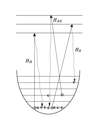
FIG. 1.: The geometry of the scattering arrangement from trapped atoms. The filled ellipsoid represents the atomic cloud with dimensions $L$ and $W$. Incident pump field comes in along the short axis of the trap, while the geometry favors the emission to be along the long axis of the trap. Momentum conservation of the absorption and the subsequent emission of photons results in the recoil of trapped atoms into a wavepacket state parametrized by $\vec{q}$.

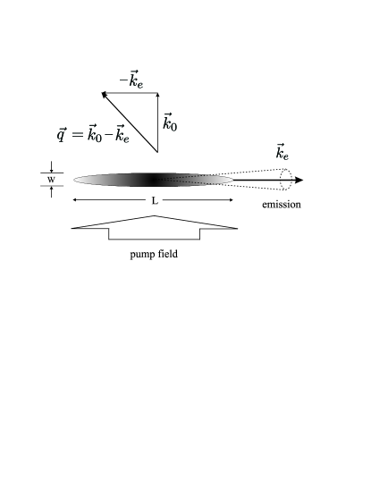
FIG. 2.: The diagram for Rayleigh, Raman Stokes and anti-Stokes scattering among the motional states of trapped atoms. The solid lines denote pump photons while dotted curve lines are for scattered photons. Solid dots denote the presence of an atom, and hollow dots denote the absence of atoms due to scattering out of certain motional states.

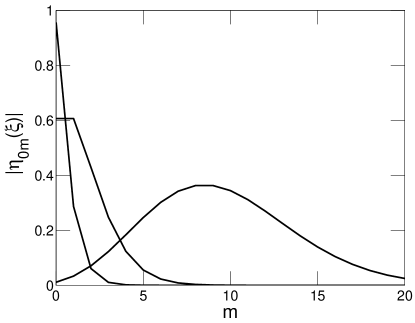
FIG. 3.: Typical values of the Franck-Condon factor $|\eta_{0,n}(\xi)|$ for $\xi=0.3,1,$ and $3$.

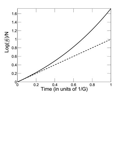
FIG. 4.: Comparison of different growth curves ${\cal G}_{\vec{q}}(t)$ for an initial motional ground state condensate with different statistics. Dashed line is for the Fock state and solid line is for the coherent state. Semi-classical treatment also predicts a growth same with the Fock state result

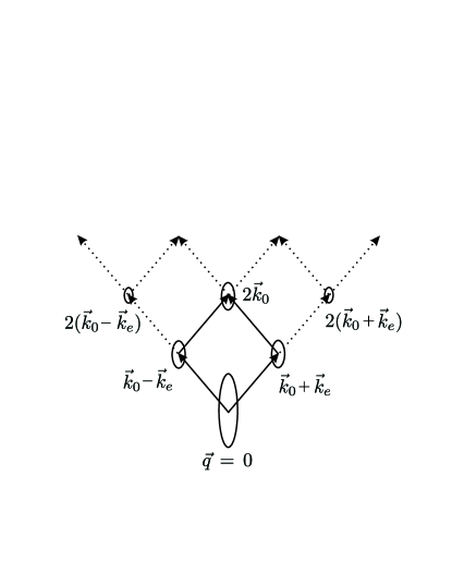
FIG. 5.: The lattice of strongly coupled atomic side modes. Solid lines show the diamond shaped unit cell with cascade dynamics.

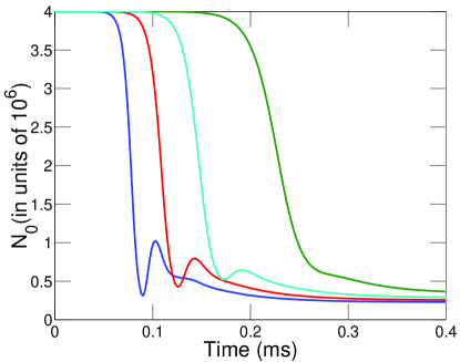
FIG. 6.: The decay of condensate population.

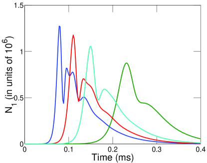
FIG. 7.: The atomic population dynamics for the first side mode(s).

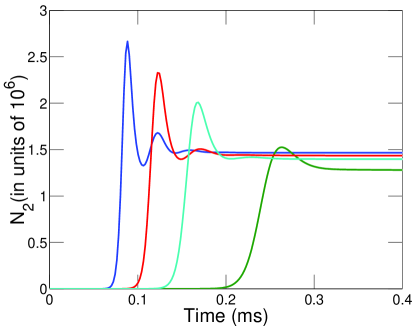
FIG. 8.: The same as in Fig. 6 but for the second side mode.

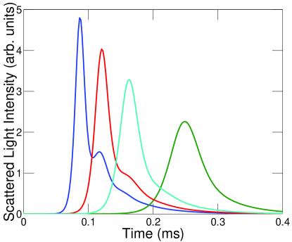
FIG. 9.: The intensity of scattered photons around one of the end firing modes.

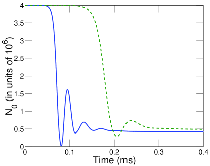
FIG. 10.: The decay of condensate population.

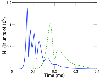
FIG. 11.: The atomic population dynamics of the first side mode(s).

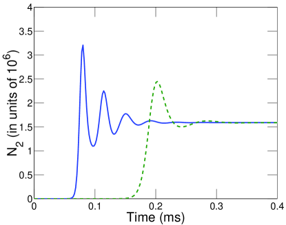
FIG. 12.: The same as in Fig. 8 but for the second side mode.

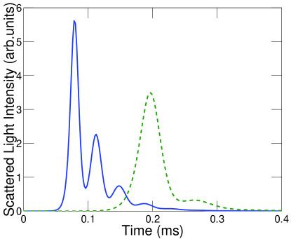
FIG. 13.: The intensity of scattered field intensity around one of the end firing modes.

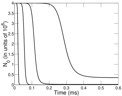
FIG. 14.: The decay of the condensate within a Markov approximation for scattered light.

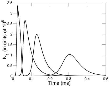
FIG. 15.: The evolution of the first side mode(s) within a Markov approximation for scattered light.

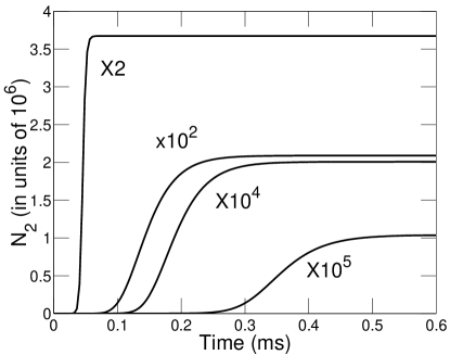
FIG. 16.: The growth of second side mode within a Markov approximation for scattered light. Curves are magnified for better view.

REFERENCES

- [1] M. H. Anderson, J. R. Ensher, M. R. Matthews, C. E. Wieman, and E. A. Cornell, Science 269, 198 (1995); K. B. Davis, M. -O. Mewes, M. R. Andrews, N. J. van Druten, D. S. Durfee, D. M. Kurn, and W. Ketterle, Phys. Rev. Lett. 75, 3969 (1995); C. C. Bradley, C. A. Sackett, J. J. Tollett, and R. G. Hulet, ibid 75, 1687 (1995); 79, 1170 (1997).
- [2] E. A. Burt, R. W. Ghrist, C. J. Myatt, M. J. Holland, E. A. Cornell, and C. E. Wieman, Phys. Rev. Lett. 79, 337 (1997); M. R. Andrews, C. G. Townsend, H.-J. Miesner, D. S. Durfee, D. M. Kurn, W. Ketterle, Science 275, 637 (1997).
- [3] L. Deng, E. W. Hagley, J. Wen, M. Trippenbach, Y. Band, P. S. Julienne, J. E. Simsarian, K. Helmerson, S. L. Rolston, and W. D. Phillips, Nature 398, 218 (1999).
- [4] S. Inouye, A. P. Chikkatur, D. M. stamper-Kurn, J. Stenger, D. E. Pritchard and W. Ketterle, Science 285, 571 (1999).
- [5] S. Inouye, T. Pfau, S. Gupta, A. P. Chikkatur, A. Görlitz, D. E. Pritchard, and W. Ketterle, Nature 402, 641 (1999).
- [6] M. G. Moore and P. Meystre, Phys. Rev. Lett. 83, 5202 (1999).
- [7] E. V. Goldstein and P. Meystre, Phys. Rev. A 59, 3896 (1999).
- [8] J. Javanainen and J. Ruostekoski, Phys. Rev. A 52, 3033 (1995).
- [9] L. You, M. Lewenstein, and J. Cooper, Phys. Rev. A 51, 4712 (1995).
- [10] M. G. Moore, O. Zobay, and P. Meystre, Phys. Rev. A 60, 1491 (1999).
- [11] J. Stenger, S. Inouye, A. P. Chikkatur, D. M. Stamper-Kurn, D. E. Pritchard, and W. Ketterle, Phys. Rev. Lett. 23, 4569 (1999).
- [12] M. Kozuma, L. Deng, E. W. Hagley, J. Wen, R. Lutvak, K. Helmerson, S. L. Rolston, and W. D. Phillips, Phys. Rev. Lett. 82, 871 (1999).
- [13] J. J. Hopfield, Phys. Rev. 112, 1555 (1958).
- [14] R. Bonifacio and L. A. Lugiato, Phys. Rev. A 11, 1507 (1975).
- [15] C. W. Gardiner, Phys. Rev. A 56, 1414 (1997).
- [16] D. Polder, M. F. H. Schuurmans, and Q. H. F. Vrehen, Phys. Rev. A 19, 1192 (1979).
- [17] N. Skribanowitz, I. P. Herman, J. C. MacGillivray, and M. S. Feld, Phys. Rev. Lett. 30, 309 (1973).
- [18] R. Bonifacio, G. R. M. Robb, and B. W. J. McNeil, Phys. Rev. A 56, 912 (1997).
- [19] H. M. Gibbs, Q. H. F. Vrehen, and H. M. J. Hikspoors, Phys. Rev. Lett. 39, 547 (1977).
- [20] C. M. Bowden and C. C. Sung, Phys. Rev. A 18, 1558 (1978).
- [21] C. M. Bowden and C. C. Sung, Phys. Rev. A 20, 2033 (1979).
- [22] L.You, J. Cooper, and M. Trippenbach, J. Opt. Soc. Am. B 8, 1139 (1990).
- [23] Quantum Theory of the Optical and Electronic Properties of Semiconductors, H. Haug and S. W. Koch, (World Scientific, Singapore, 1990).
- [24] R. bonifacio and A.L.Lugiato, Phys. Rev. A 12, 587 (1975); AV Andreev, JETP 45, 734 (1977); AV Andreev, NA Enaki, and Yu A Ilinskii, JETP 60, 229 (1984); Cooperative Effects in Optics: Superradiance and phase transitions, AV Andreev, VI Emel’yanov, and Yu A Ilinskii, (IOP publishing, Bristol, 1993).
- [25] E. A. Watson, H. M. Gibbs, F. P. Mattar, M. Cormier, Y. Claude, S. L. McCall, M. S. Feld, Phys. Rev. A 27, 1427 (1983).
- [26] F. P. Mattar and C. M. Bowden, Phys. Rev. A 27, 345 (1983).
- [27] L. Mandel and E. Wolf, Optical coherence and Quantum Optics, (Cambridge University Press, New York, 1995), p847.
- [28] D. J. Heinzen, J. E. Thomas, and M.S. Feld, Phys. Rev. Lett. 54, 677 (1985).
- [29] A. Kumarakrishnan and X. L. Han, Opt. Commun. 109, 348 (1994).
- [30] A. Aspect, J. Dalibard, and G. Roger, Phys. Rev. Lett. 49, 1804 (1982).
- [31] A. Kumarakrishnan and X. L. Han, Phys. Rev. A 58, 4153 (1998).