Light Scattering from Nonequilibrium Concentration Fluctuations in a Polymer Solution

Abstract

We have performed light-scattering measurements in dilute and semidilute polymer solutions of polystyrene in toluene when subjected to stationary temperature gradients. Five solutions with concentrations below and one solution with a concentration above the overlap concentration were investigated. The experiments confirm the presence of long-range nonequilibrium concentration fluctuations which are proportional to $(\nabla T)^{2}/k^{4}$, where $\nabla T$ is the applied temperature gradient and $k$ is the wave number of the fluctuations. In addition, we demonstrate that the strength of the nonequilibrium concentration fluctuations, observed in the dilute and semidilute solution regime, agrees with theoretical values calculated from fluctuating hydrodynamics. Further theoretical and experimental work will be needed to understand nonequilibrium fluctuations in polymer solutions at higher concentrations.

I Introduction

Density and concentration fluctuations in fluids and fluid mixtures can be investigated experimentally by light-scattering techniques. The nature of these fluctuations when the system is in equilibrium is a subject well understood[1, 2]. Here we shall consider fluctuations in nonequilibrium steady states (NESS), when an external and constant temperature gradient is applied, while the system remains in a hydrodynamically quiescent state. That is, we shall deal with fluctuations that are intrinsically present in thermal nonequilibrium states in the absence of any convective instabilities. Such fluctuations have received considerable attention during the past decade[3]. It was originally believed that, because of the existence of local equilibrium in NESS, the time correlation function of the scattered-light intensity would be the same as in equilibrium, but in terms of spatially varying thermodynamic and transport properties corresponding to the local value of temperature. However, it has been demonstrated that qualitative differences do appear. The first complete expression for the spectrum of the nonequilibrium fluctuations in a one-component fluid subjected to a stationary gradient was obtained by Kirkpatrick et al.[4] by using mode-coupling theory. They showed that the central Rayleigh line of the spectrum would be substantially modified as a result of the presence of a temperature gradient. Because of a coupling between the temperature fluctuations and the transverse-velocity fluctuations through the temperature gradient, spatially long-range nonequilibrium temperature and viscous fluctuations appear, modifying the Rayleigh spectrum of the scattered-light intensity. Their results were subsequently confirmed on the basis of fluctuating hydrodynamics[5, 6]. The effect is largest for the transverse-velocity fluctuations in the direction of the temperature gradient which corresponds to the situation that the scattering wave vector, ${\bf k}$, is perpendicular to the temperature gradient $\nabla T$, which configuration will be assumed throughout the present paper. In that case, the strengths of the nonequilibrium temperature and viscous fluctuations are predicted to be proportional to $(\nabla T)^{2}/k^{4}$. The dependence on $k^{-4}$ implies that, in real space, the nonequilibrium correlation functions become long ranged[3, 7]. The spatially long-range nature of the correlation functions in NESS is nowadays understood as a general phenomenon arising from the violation of the principle of detailed balance[3, 8]. Experimentally, the long-range nature of the nonequilibrium fluctuations can be probed by light-scattering measurements at small wave numbers $k$, i.e. at small scattering angles $\theta$. Such experiments have been performed in one-component liquids and excellent agreement between theory and experiments has been obtained[9, 10].

In binary systems, the situation is a little more complicated. In liquid mixtures or in polymer solutions a temperature gradient will induce a concentration gradient through the Soret effect. This induced concentration gradient is parallel to the temperature gradient and has the same or opposite direction depending on the sign of the Soret coefficient, $S_{T}$. In this case, nonequilibrium fluctuations appear, not only because of a coupling between the temperature fluctuations and the transverse-velocity fluctuations through the temperature gradient, but also because of a coupling between the concentration fluctuations and the transverse-velocity fluctuations through the induced concentration gradient. The nonequilibrium Rayleigh-scattering spectrum has been calculated for binary liquid mixtures, both on the basis of mode-coupling theory[11] and on the basis of fluctuating hydrodynamics[12], with identical results. In liquid mixtures in thermal nonequilibrium states not only nonequilibrium temperature and nonequilibrium viscous fluctuations, but also nonequilibrium concentration fluctuations exist. The strengths of all three types of nonequilibrium fluctuations are again predicted to be proportional to $(\nabla T)^{2}/k^{4}$. The theory was extended by Segrè et al.[13, 14] to include the effects of gravity and by Vailati and Giglio[15] to include time-dependent nonequilibrium states. The nature of the nonequilibrium fluctuations in the vicinity of a convective instability has also been investigated[14, 16, 17], in which case the nonequilibrium modes become propagative. The influence of boundary conditions, which may become important when ${\bf k}$ is parallel to $\nabla T$, was considered by Pagonabarraga et al.[18].

Experiments have been performed to study nonequilibrium fluctuations in liquid mixtures[10, 19, 20, 21]. The three types of nonequilibrium fluctuations have been observed in liquid mixtures of toluene and n-hexane[10, 19, 20] and the strength of all three types of nonequilibrium fluctuations were indeed proportional to $(\nabla T)^{2}/k^{4}$, as expected theoretically. Initially, it seemed that also the prefactors of the amplitudes of these nonequilibrium fluctuations were in agreement with the theoretical predictions[19]. However, a definitive assessment was hampered by a lack of reliable experimental information on the Soret coefficient[19, 20]. To our surprise, subsequent accurate measurements of the Soret coefficient of liquid mixtures of toluene and n-hexane obtained both by Köhler and Müller[22] and by Zhang et al.[23] yielded values for the Soret coefficient that were about 25% lower than the values needed to explain the quantitative magnitude of the amplitudes of the observed nonequilibrium fluctuations[23]. Subsequent measurements of the nonequilibrium concentration fluctuations in a mixture of aniline and cyclohexane, obtained by Vailati and Giglio[21] did not have sufficient accuracy to resolve this issue.

As an alternative approach, we decided to investigate nonequilibrium concentration fluctuations in a polymer solution. In a polymer solution the same nonequilibrium enhancement effects are expected to exist, but the mass-diffusion coefficient, $D$, in this case is several orders of magnitude lower than in ordinary liquid mixtures. In addition, the Soret coefficient is two orders of magnitude larger that the Soret coefficient of ordinary liquid mixtures[24]. These two facts, as discussed below, simplify the theory because, as also happens in an equilibrium polymer solution, the concentration fluctuations become dominant and they are readily observed by light scattering. Both the data acquisition and the data analysis become much easier in this case. Thus a polymer solution would seem to be an ideal system to further investigate nonequilibrium concentration fluctuations.

For this purpose we have selected solutions of polystyrene in toluene, for which reliable information on the thermophysical properties is available. We have performed small-angle Rayleigh-scattering experiments in polystyrene-toluene solutions subjected to various externally applied temperature gradients. A summary of our results has been presented in a Physical Review Letter[25]. In the present paper we provide a full account of the experiment and of the analysis of the experimental data.

II Theory

A theory specifically developed for the fluctuations in polymer solutions in thermal nonequilibrium states is not yet available in the literature. However, for polymer solutions in the dilute and semidilute solution regime, as long as entanglement effects can be neglected, it should be possible to use the same fluctuating hydrodynamics equations as those for ordinary liquid mixtures. As mentioned in the introduction, the complete expression for the Rayleigh spectrum of a binary liquid in the presence of a stationary temperature gradient was evaluated by Law and Nieuwoudt[12]. The dynamic structure factor contains three diffusive modes. The decay rate $\lambda_{\nu}=\nu k^{2}$ of one of these modes is determined by the kinematic viscosity $\nu$; this mode disappears in thermal equilibrium, i.e. when $\nabla T\rightarrow 0$. The other two modes are also present in the Rayleigh spectrum of a liquid mixture in equilibrium and have the decay rates $\lambda_{\pm}$ given by:

$$\lambda_{\pm}={k^{2}\over 2}(D_{T}+{\cal D})\mp{k^{2}\over 2}\left[(D_{T}+{\cal D})^{2}-4D_{T}D\right]^{1/2},$$ (1)

where $D_{T}$ is the thermal diffusivity, $D$ the binary mass-diffusion coefficient, in the case of a polymer solution to be referred to as collective diffusion coefficient[24], and where

$${\cal D}=D(1+\epsilon)$$ (2)

with

$$\epsilon=T~{}{[S_{T}~{}w(1-w)]^{2}\over c_{P,c}}~{}\left({\partial\mu\over\partial w}\right)_{p,T}.$$ (3)

In Eq. (3) $w$ is the concentration expressed as mass fraction of the polymer, $c_{P,c}$ the isobaric specific heat capacity of the solution at constant concentration, and $\mu$ is the difference between the chemical potentials per unit mass of the solvent and the solute. As usual, the Soret coefficient, $S_{T}$, specifies the ratio between temperature and concentration gradients and it is defined through the steady-state phenomenological equation:

$$\nabla w=-S_{T}~{}w~{}(1-w)~{}\nabla T.$$ (4)

The two modes with decay rates $\lambda_{\pm}$ incorporate a coupling between temperature and concentration fluctuations. This coupling becomes important in compressible fluid mixtures near a critical locus[26]. However, when $\epsilon\ll 1$, the dynamic structure factor of a binary system in NESS consists of just three exponentials with decay rates given by:

$$\lambda_{\nu}=\nu k^{2},~{}\lambda_{+}=D_{T}k^{2},~{}\lambda_{-}=Dk^{2}.$$ (5)

Physically, it means that the temperature gradient $\nabla T$ induces nonequilibrium viscous fluctuations appearing as a new term in the Rayleigh spectrum and it leads to nonequilibrium enhancements of the temperature and concentration fluctuations.

The condition $\epsilon\ll 1$ is always fulfilled in the low-concentration limit[2]. But for some liquid mixtures $\epsilon$ is also small at all concentrations. For instance, in an equimolar mixture of toluene and n-hexane Segrè et al. found $\epsilon\approx 0.028$. For the dilute polymer solutions considered in the present paper, $\epsilon\approx 0.010$. Hence, the approximations implying the presence of three diffusive modes with the simple decay rates given by Eq. (5) are even more justified for a polymer solution than for the liquid mixtures studied in previous papers[10, 19].

Furthermore, in ordinary polymer solutions $D/D_{T}\approx 5\times 10^{-4}$; such a small value simplifies the analysis of the concentration fluctuations, because the decay in the time correlation function coming from the concentration mode (decay rate $\lambda_{-}$) will be well separated from the decays of the modes with decays rates $\lambda_{\nu}$ and $\lambda_{+}$. Actually, for the small angles employed in our experiments, the decay time of the $\lambda_{-}$ mode is typically 0.5-1.5 s, whereas the decay times of the other two modes are around $10^{-4}-10^{-5}$ s. In addition, for a dilute polymer solution, the Rayleigh factor ratio, that determines the ratio of the scattering intensities of the concentration fluctuations and the temperature fluctuations[19], is much larger than unity so that the contributions of temperature fluctuations are negligibly small in practice. Moreover, when the experimental correlograms are analyzed beginning at $10^{-2}$ s, viscous and temperature fluctuations have already decayed. This kind of approximation is usually assumed in the theory of light scattering from polymer solutions in equilibrium states[1].

In conclusion, for heterodyne light-scattering experiments in sufficiently dilute polymer solutions, the expression for the time-dependent correlation function of the scattered light becomes:

$$C(k,t)=C_{0}[1+A_{c}({\bf k},\nabla T)]e^{-Dk^{2}t},$$ (6)

where $C_{0}$ is the signal to local-oscillator background ratio representing the amplitude of the correlation function in thermal equilibrium. In Eq. (6) the term $A_{c}({\bf k},\nabla T)$ represents the nonequilibrium enhancement of the concentration fluctuations. This term is anisotropic and depends on the scattering angle. When ${\bf k}\perp\nabla T$, $A_{c}$ reaches a maximum given by:

$$A_{c}(k,\nabla T)=A^{*}_{c}(w)~{}{(\nabla T)^{2}\over k^{4}},$$ (7)

where the strength of the enhancement, $A^{*}_{c}(w)$, is given by[10, 12, 14, 19]:

$$A^{*}_{c}(w)={\left[w(1-w)\right]^{2}{S_{T}}^{2}\over\nu D}~{}\left({\partial\mu\over\partial w}\right)_{p,T}~{}\left[1+2{D\over D_{T}}(1+\zeta)\right],$$ (8)

where $\zeta$ is a dimensionless correction term related to the ratio of $(\partial n/\partial T)_{P,w}$ and $(\partial n/\partial w)_{P,T}$. As mentioned earlier for the polymer solutions to be considered, $D/D_{T}$ is of the order of $5\times 10^{-4}$, so that the correction term inside the square brackets can be neglected in practice. Hence, the expression for $A^{*}_{c}(w)$ reduces to:

$$A^{*}_{c}(w)={\left[w(1-w)\right]^{2}{S_{T}}^{2}\over\nu D}~{}\left({\partial\mu\over\partial w}\right)_{p,T}.$$ (9)

The dependence of the nonequilibrium enhancement $A_{c}$ of the concentration fluctuations on $k^{-4}$ indicates that the correlations in real space are long ranged. Actually, a $k^{-4}$ dependence in Fourier space corresponds to a linear increase of the correlation function in real space [7]. The rapid increase of the strength of the nonequilibrium fluctuations with decreasing values of the wavenumber will saturate for sufficiently small $k$ due to the presence of gravity. The gravity effect was predicted by Segrè et al.[13] and has been confirmed by some beautiful experiments of Vailati and Giglio[21].

Our set of working equations, Eqs. (6), (7) and (9), can be also deduced from the theory of Vailati and Giglio for nonequilibrium fluctuations in time-dependent diffusion processes[15]. In that paper only concentration and velocity fluctuations are considered around a nonequilibrium time-dependent state. By applying an inverse Fourier transform to Eq. (25) of Vailati and Gilio[15], we obtain for the autocorrelation function of the concentration fluctuations for ${\bf k}\perp\nabla w$:

$$\langle\delta w\delta w^{*}\rangle=S(k)\exp\left[-Dk^{2}t\left(1-{R(k)\over R_{c}}\right)\right],$$ (10)

where $R(k)/R_{c}$ is the Rayleigh-number ratio, which accounts for the effects of gravity and is defined in Eq. (22) of Vailati and Giglio[15]. $S(k)$ is the static structure factor, defined in Eq. (26) of the same paper. It should be noticed that, for consistency, in our Eq. (10) we have used the symbol $w$ instead of the $c$ used by Vailati and Giglio. Both symbols have the same meaning, as it is stated after Eq. (2) of Vailati and Giglio that: ”$c$ is the weight fraction of the denser component”. Thus Eq. (26) of Vailati and Giglio for the static structure factor $S(k)$ can be written as:

$$S(k)={k_{B}T\over 16\pi^{4}\rho}~{}\left({\partial w\over\partial\mu}\right)_{p,T}~{}{1\over 1-R(k)/R_{c}}~{}\left[1+{(\nabla w)^{2}\over\nu Dk^{4}}~{}\left({\partial\mu\over\partial w}\right)_{p,T}~{}\right].$$ (11)

The derivation of Vailati and Giglio[15] was originally developed for time-dependent isothermal diffusion processes in the presence of gravity, where only concentration gradients are present. The validity of this theory for stationary nonequilibrium states is obvious, and we can consider $\nabla w$ to be constant, neglecting the weak dependence on space and time considered by Vailati and Giglio[15]. Neglecting gravity effects is equivalent to assuming that the Rayleigh-number ratio is almost zero, $R(k)/R_{c}\approx 0$, as can be easily shown from Eq. (22) in the paper of Vailati and Giglio[15]. Introducing Eq. (4) into Eq. (11) and neglecting $R(k)/R_{c}$, one readily verifies that Eqs. (10) and (11) are equivalent to Eqs. (7) and (9).

We note that Eqs. (6), (7) and (9) can also be obtained as a limiting case of the equations derived by Schmitz for nonequilibrium concentration fluctuations in a colloidal suspension [27]. Schmitz considered a colloidal suspension, in the presence of a constant gradient, $\nabla\phi$, in the volume fraction, $\phi$, of the colloidal particles, maintained against diffusion by continuous pumping of solvent between two semipermeable and parallel walls. The relevant expression is Eq. (7.7) in the article of Schmitz[27], which gives the dynamic structure factor, $S(k,\omega)$, of the nonequilibrium concentration fluctuations as a function of the wavenumber $k$ and the frequency $\omega$. The expression obtained by Schmitz includes non-local and memory effects due to the large particle sizes in comparison with the scattering wavelength. The non-local and memory effects cause the transport coefficients to depend on the frequency and the wave number. In our case these effects can be neglected, because the polymer molecules are much smaller that the colloidal particles considered by Schmitz and the condition $kR_{\rm g}\ll 1$, where $R_{\rm g}$ is the radius of gyration, is fulfilled. With this simplification the original expression obtained by Schmitz reduces to:

$$S(k,\omega)=S(k)~{}[1+A_{c}]~{}{2Dk^{2}\over\omega^{2}+(Dk^{2})^{2}},$$ (12)

where $A_{c}$ is given by:

$$A_{c}={w^{2}\over\nu D}~{}\left({\partial\mu\over\partial w}\right)_{p,T}~{}\left({\nabla\phi\over\phi}\right)^{2}~{}{1\over k^{4}}.$$ (13)

In deriving Eq. (13) we have used the relationship between pumping rate and volume fraction gradient, as given by Eqs. (7.6) and (7.11) in the paper of Schmitz[27]. We have also converted the various concentration units used by Schmitz: $n$ which is the number of particles per unit volume ($n=\rho/w~{}m_{\rm p}$) and $c$ which is the number of particles per unit mass ($c=w/m_{\rm p}$), $\rho$ being the density of the suspension and $m_{\rm p}$ the mass of one particle. Furthermore, we are using the difference between solvent and solute chemical potentials per unit mass, whereas in the paper of Schmitz $\mu$ is the difference in chemical potentials per particle.

Although the theory of Schmitz for the nonequilibrium concentration fluctuations was derived for the case that the concentration gradient is produced by a solvent flow, the results will be applicable to NESS under a constant temperature gradient. Since the solvent flow does not appear explicitly in Eq. (13), we may also apply the equation to a system subjected to a stationary volume-fraction gradient caused by other driving forces, such as a temperature gradient. For our polymer solutions $(\nabla\phi/\phi)^{2}\approx(\nabla w/w)^{2}$, the difference being less than 0.5%. With this approximation and by using Eq. (4), it is straightforward to show the equivalence of the theory for nonequilibrium concentration fluctuations in a colloidal suspension and in a polymer solution, independent of whether the concentration gradient is established by solvent pumping or induced by a temperature gradient.

III Experimental Method

The polystyrene used to prepare the polymer solutions was purchased from the Tosoh Corporation (Japan); it has a mass-averaged molecular weight $M_{W}=96,400$ and a polydispersivity of 1.01, as specified by the manufacturer[24]. The solvent toluene was Fisher certified reagent purchased from Baker Chemical Co. with a stated purity of better than 99.8%. By using the correlation proposed by Noda et al.[28, 29], $\langle R_{\rm g}^{2}\rangle=1.38\times 10^{-2}M_{W}^{1.19}$, the radius of gyration, $R_{\rm g}$, and the overlap concentration, $w^{*}$, for this polymer in toluene solutions may be estimated as $R_{\rm g}\approx 11.0$ nm and $w^{*}\approx 3.1\%$, respectively. Therefore, for the viscoelastic and entanglement effects to be negligible, the concentrations employed in this work should not be much higher than $3.1\%$. Five polystyrene/toluene solutions below $w^{*}$ and one slightly above $w^{*}$ were prepared gravimetrically as described by Zhang et al.[24]. To assure the homogeneity of the mixture, the solutions were agitated (magnetic stirrer or shaking by hand)for at least one hour before further use.

The light-scattering experiments were performed with an apparatus specifically designed for small-angle Rayleigh scattering in an horizontal fluid layer subjected to a vertical temperature gradient[10]. A diagram of the optical cell is shown in Fig. 1. The following paragraphs will describe the apparatus in detail, and references to the symbols in Fig. 1 will be used. The polymer solution in the actual light-scattering cell (E) is confined by a circular quartz ring (D) that is sandwiched between top and bottom copper plates (A and F, respectively). The cell is filled through two stainless steel capillary tubes (G) which had been soldered into holes in the top and bottom plates. The inner and the outer diameters of the quartz ring (D) are 1.52 cm and 2.05 cm, respectively. Two identical optical windows (B) are used for letting a laser beam pass through the liquid solution. Both windows are cylindrical and made from sapphire because of the relatively high thermal conductivity of this material. The windows are epoxied into the centers of the top and the bottom copper plates by a procedure similar to the one described by Law et al.[30]. Once the optical windows are installed, the top and bottom copper plates are sealed against the quartz ring by indium O-rings. To avoid heat conduction from the upper to the lower plate other than through the liquid, the two copper plates are held together by teflon screws (not shown in the figure). The tension of these teflon screws was adjusted to set the flat surfaces of the optical windows parallel to within 10 seconds of arch. This was accomplished by passing a laser beam through the cell and monitoring the interference pattern of the reflected beams from the inner surfaces of the windows while the screws were fastened. Once the cell was mounted, the distance $d$ between the windows was accurately determined by measuring the angular variation of these interference fringes. The result was $d=(0.118\pm 0.005)$ cm. This value was confirmed by also measuring the separation with a cathetometer.

Since the nonequilibrium enhancement of the fluctuations given by Eq. (7) depends on $k^{-4}$, small scattering angles are required to obtain measurable values of $A_{c}$; in practice scattering angles $\theta$ between 0.4^∘ and 0.9^∘ were used. A major difficulty with such small-angle experiments is the presence of strong static scattering from the optical surfaces. To reduce the background scattering, we needed very clean windows. The optical surfaces of the windows and the other optical components of the experimental arrangement were cleaned by applying first a Windex solution and then acetone with cotton swabs. Moreover, we employ thick cell windows to remove the air-window surfaces from the field of view of the detector. In addition, the outer surface of the windows and the other optical surfaces were broad-band (488-623 nm) anti-reflection coated (CVI Laser Corporation), to reduce the back reflections and forward scattering intensity. As a result of these efforts, we obtained high enough signal to background ratios to allow accurate measurements of the scattered-light intensities.

To observe the intrinsic nonequilibrium fluctuations, it is essential to avoid any convection in the liquid layer. This is accomplished by heating the horizontal fluid layer from above. Furthermore, bending and defocusing of the light beam due to the refractive-index gradient induced by the temperature gradient could cause serious limitations in the resolution of the angles. This difficulty is avoided by employing a vertical incident light beam, parallel to the temperature gradient. To eliminate stray deflections caused by air currents near the cell, the whole assembly is covered by a plexiglass box with a small hole at the top to let the laser beam pass through.

The temperature at the top plate was maintained by a computer controlled resistive heater winding (C). The temperature at the bottom plate is controlled by circulating constant-temperature fluid from a Forma Model 2096 bath through channels in the base of the cell (I), which is in good thermal contact with the bottom plate. With these devices, the temperatures of both the hot and cold plates can be held constant to within $\pm$20 mK. These temperatures remain fixed over the collection time of any experimental run. Temperatures of both plates are monitored by thermistors inserted in holes (H) next to the sample windows and deep enough to be located very close to the liquid layer. Due to the relatively high thermal conductivity of the sapphire windows and the symmetry of the arrangement, the lateral temperature gradients are small. Numerical modeling of the thermal conduction process yields negligible differences between the measured temperature gradient and the actual temperature gradient between the windows.

A coherent beam ($\lambda=632.8$ nm) from a 6 mW stabilized cw He-Ne laser is focused with a 20 cm focal length lens onto the polymer solution in the scattering cell. The scattering angle, $\theta$ is selected with a small pinhole (500 $\mu$m) located 197 mm after the cell. The collecting pinhole is placed in a plane orthogonal to the transmitted beam. The distance between the point where the beam hits the collection plane and the pinhole was carefully measured with a vernier micrometer scale.

In the original light-scattering experiments of Law et al.[9] in NESS of a one-component liquid, the scattering wave number, $k$, was determined from equilibrium light-scattering measurements and the known value of the thermal diffusivity, $D_{T}$. In the present experiments we have determined $k$ by directly measuring the scattering angle $\theta$. Since the intensities of the nonequilibrium fluctuations depend on $k^{-4}$, the measurement of $k$ has to be done with considerable accuracy. By working out the ray tracing problem, taking into account refraction at the two window surfaces, we can deduce the scattering angle, $\theta$, from the location of the pinhole relative to that of the transmitted beam For this calculation the thickness of the bottom window, the distance from the window to the collecting plane, the refractive index of the window and the refractive index, $n$, of the solution are needed. It was assumed that the scattering volume is in the middle of the cell, but since the cell is very thin the possible corrections to this assumption are negligible. The distances were measured with an accuracy of $\pm 0.05$ cm. The value 1.7660 of the refractive index of the window at the wavelength $\lambda$ of the incident light was obtained from the manufacturer. The refractive index, $n$, of the polystyrene solutions as a function of the polymer concentration at 25^∘C was measured with a thermostated Abbé refractometer as described by Zhang et al.[24]. For the polystyrene solutions considered in the present paper the refractive index can be represented by[24]:

$$n(w)=1.490~{}49+0.092~{}20\cdot w+0.025~{}56\cdot w^{2}.$$ (14)

The scattering wave number $k$ is related to the scattering angle $\theta$ through the Bragg condition $k={4\pi n\over\lambda}\sin({\theta/2})$, where $\lambda$ is the wavelength of the incident light. Taken into account the experimental errors in the different magnitudes relevant to the calculation, we were able to determine $k$ with an accuracy of 1.5%.

As discussed in section II, we want to investigate the concentration fluctuations, which yield the dominant contribution to the Rayleigh spectrum. Since typical decay times for this mode at the small angles employed are always larger than 0.5 s, we are interested in the experimental correlograms for times starting around 10^-2 s. Since this value is well above the region where photomultiplier (PM) afterpulsing effects are important, unlike in previous work[9, 19], cross-correlation was not necessary for our measurements. This simplifies the experimental arrangement. The light exiting through the pinhole is focused, through corresponding optics, onto the field selecting pinhole in front of a single PM. The signal from the PM and the corresponding discriminator is analyzed with an ALV-5000 multiple tau correlator.

IV Experimental Procedure and Experimental Results

Rayleigh-scattering measurements were obtained for six different solutions of polystyrene in toluene, with concentrations $w$ in weight fraction ranging from 0.50% to 4.00%. For each solution, the measurements were performed at three to five scattering angles, ranging from 0.4^∘ to 0.9^∘, which corresponds to scattering wave numbers $k$ ranging from 900 cm^-1 to 2000 cm^-1. These small angles cause the stray light from window-surface scattering to be dominant, assuring that the measurements are in the heterodyne regime. Hence, the light scattered from the inner surfaces of the windows plays the role of a local oscillator and provides the background with which our signal, the light scattered from the polymer solution, is mixed.

Before starting the experiments, the light-scattering cell was carefully cleaned by flushing the cell with pure toluene for at least one hour. Next, a gentle stream of nitrogen gas was continuously directed through the cell to dry the inner walls and to remove dust particles. After this cleaning procedure the polymer solution was introduced into the cell through a 0.5 $\mu$m millipore Millex HPLC teflon filter. We have been careful to remove bubbles from the light-scattering cell while we were filling it with the polymer solution. This cleaning and filling procedure was repeated each time the concentration of the solution inside the cell was changed.

It should be noted that a portion of the same polymer solution was introduced into an optical beam-bending cell for measuring the diffusion coefficient, $D$, and the Soret coefficient, $S_{T}$, of the solutions as described by Zhang et al.[24]. These independent measurements of the diffusion and Soret coefficients will be used to compare the results of our light-scattering measurements with the theoretical predictions. In the case of polymer solutions it is especially important to have independent measurements of these quantities for the same polymer/solvent system because, as commented below, there is a sizable dispersion in the literature data, mainly caused by the dependence of these coefficients on parameters difficult to control, such as the polydispersity of the sample.

Once the cell was filled with a polystyrene solution with known polymer concentration, we started the experiments by setting the temperature of the top and the bottom plates of the cell at 25^∘C. A light-scattering angle was then selected with the collection pinhole, and the distance in the collection plane between the pinhole and the center of the transmitted forward-beam spot was measured accurately. As already mentioned, this procedure, with the corresponding calculations, yielded scattering wave vectors $k$ with an accuracy of 1.5%. Once a scattering angle was selected, the optics was arranged to focus the light exiting through the collecting pinhole into the field-stop pinhole at the PM. When the temperature of the polymer solution had stabilized, we used the ALV-5000 to collect at least ten equilibrium light-scattering correlation functions, with the polymer solution in thermal equilibrium at 25^∘C. The photon count rate of these measurements ranged from 0.3 to 2.5 MHz, depending on the run. Each correlation lasted from 30 to 60 minutes, with signal to background ratios from $1\times 10^{-4}$ to $1\times 10^{-3}$. These small signal to background ratios confirm that our measurements are in the heterodyne regime. After having completed the measurements with the polymer solution in thermal equilibrium, we applied various values of the temperature gradient to the polymer solution by increasing and decreasing the temperatures of the top and bottom plates symmetrically, so that all experimental results correspond to the same average temperature of 25^∘C. The maximum temperature difference employed was 4.1^∘C, which corresponds to a maximum temperature gradient of 34.6 K cm^-1. The variation in the thermophysical properties of the solutions is negligible in this small temperature interval, and the property values corresponding to 25^∘C have been used for the calculations. After changing the temperatures, we waited at least two hours, to be sure that the concentration gradient was fully developed. Then, for each value of the temperature gradient, about six correlograms were taken. In Fig. 2, typical experimental light-scattering correlograms, obtained with the ALV-5000 correlator at $k=1030$ cm^-1 are shown for the solution with polymer mass fraction $w=2.50\%$, as a function of the temperature gradient $\nabla T$. The figure shows the well sampled amplitude of the correlation at short times for the correlograms. A simple glance at Fig. 2 confirms that the amplitude of the correlation function increases with increasing values of the temperature gradient $\nabla T$.

The correlograms, in the range from 10^-2 s to 1 s, depending on the run, were fitted to a single exponential, in accordance with Eq. (6). In all cases, both in equilibrium and in nonequilibrium, very good fits were obtained. Actually, the intensity of the scattered light is observed over a range of wave numbers corresponding to the non-zero aperture of the collecting pinhole. This effect can be accounted for by representing the experimental correlation function in terms of a Gaussian convolution, as explained in previous publications[9, 10]. However, we found that the resulting corrections to the parameter values obtained from fits to a single exponential amounted to less than 1% for the present experiments and could be neglected. Hence, experimental values for the decay rate, $Dk^{2}$, and for the prefactor $C_{0}[1+A_{c}(k,\nabla T)]$ were obtained by directly fitting the time-correlation function data of the scattered light to a single exponential, as given by Eq. (6).

The experimental values obtained for the decay rates, $Dk^{2}$, for the polymer solutions at various values of the scattering wave number $k$ and the temperature gradient $\nabla T$ are presented in Table I. Each value displayed in Table I is the average from several (at least five) experimental correlograms obtained at the same conditions. The prefactor of the exponential obtained from the fitting procedure was multiplied by the average count rate during the run to get the average intensity (in 10⁶ counts/s) in each run. The dimensionless enhancement, $A_{c}$, of the concentration fluctuations at a given nonzero value of $\nabla T$ was obtained from the ratio of the nonequilibrium to the equilibrium intensities, measured at the same $k$, by means of Eq. (6). The experimental values obtained for $A_{c}$ are presented in Table II. Again, each value displayed in Table II is an average of several correlograms measured at the same conditions. The uncertainties quoted in Tables I and II represent standard deviations of the values obtained from the sets of experimental correlograms.

V Analysis of Experimental Results

A Mass-diffusion coefficient $D$

Dividing the decay rates displayed in Table I by the square of the known wave numbers, a mass-diffusion coefficient, $D$, is obtained for each $w$, $k$ and $\nabla T$. As an example, we show in Fig. 3 the values of $D$ thus obtained for the polymer solution with $w=0.50\%$ obtained from the light-scattering measurements at various values of the wave number $k$, as a function of the applied temperature gradient $\nabla T$. The horizontal line in Fig. 3 represents the weighted average value of $D$. It is readily seen that the experimental $D$ is independent of $\nabla T$, which implies that the applied temperature gradient does not affect the translational diffusion dynamics of the polymer molecules and that we indeed observed concentration fluctuations for all $\nabla T$. Figure 3 also demonstrates that $D$ is independent of the wave number $k$. Thus the decay rates in Table I are indeed proportional to $k^{2}$, which confirms the correctness of our measurements of $k$. For each concentration we determined a simple value of $D$ as an average of the experimental data obtained at various $k$ and $\nabla T$. In the averaging process the individual accuracies were taken into account. The resulting values of $D$ for the different polymer solutions are presented in Table III and displayed in Fig. 4 as a function of the polymer concentration. For this purpose we prefer to use the concentration $c$ in g cm^-3, because this unit is more widely employed in the literature for polymer solutions. To change the concentration units we used the relationship:

$$\rho(w)=0.86178+0.1794~{}w+0.0296~{}w^{2}~{}({\rm g~{}cm^{-3}}),$$ (15)

as reported by Scholte[31]. The error bars in Fig. 4 have been calculated by adding 3% of the value of $D$ to the standard deviations given in Table III, so as to account for the uncertainty in the wave number $k$. In Fig. 4 we have also plotted the values obtained by Zhang et al. for the collective diffusion coefficient of the same polymer solutions with an optical beam-bending technique[24]. This figure shows that the values obtained from the two methods for the diffusion coefficient agree within the experimental accuracy. The straight line displayed in Fig. 4 represents the linear relationship:

$$D(c)=D_{0}(1+k_{D}~{}c),$$ (16)

with the values

$$D_{0}=(4.71\pm 0.08)\times 10^{-7}~{}{\rm cm}^{2}{\rm s}^{-1},$$ (18)

and

$$k_{D}=(22\pm 2)~{}{\rm cm}^{3}{\rm g}^{-1}.$$ (19)

for the diffusion coefficient at infinite dilution, $D_{0}$, and the hydrodynamic interaction parameter, $k_{D}$, as determined by Zhang et al.[24] for the polymer solution with the same molecular mass $M_{W}=96,400$. It may be observed that the $D_{0}$ and $k_{D}$ values proposed by Zhang et al.[24] yield a satisfactory description of the dependence of our $D$ values on the concentration.

An extensive survey of literature values for $D_{0}$ and $k_{D}$ of polystyrene in toluene solutions was performed, and ten different references were examined [24, 32, 33, 34, 35, 36, 37, 38, 39, 40]. Most authors have studied the molecular weight dependence of these parameters and propose relationships which usually have the form of power laws. The results of our survey are presented in Table IV. In some cases where the scaling equations are not directly given by the authors, we have performed the corresponding fits to obtain the power-law dependence of $D_{0}$ and $k_{D}$ on $M_{W}$. All data in Table IV correspond to polystyrene in toluene at the temperature of 25^∘C. While $k_{D}$ should be nearly independent of temperature because toluene is a good solvent[39], $D_{0}$ depends on temperature through a Stokes-Einstein relation. Neglecting the dependence on temperature of the hydrodynamic radius of polystyrene in toluene[41], we represent the dependence of $D_{0}$ on the temperature, $T$, by:

$$D_{0}\propto{T\over\eta_{0}(T)},$$ (20)

where $\eta_{0}(T)$ is the viscosity of the pure solvent (toluene) as a function of temperature which can be found in the literature[41]. Equation (20) was used for making temperature corrections in cases where the values of $D_{0}$ reported in the literature had been measured at temperatures other than 25^∘C. Furthermore, we did not consider literature values measured at temperatures more than $\pm$10 K from 25^∘C. The sixth column of Table IV contains the values extrapolated to $M_{W}=96,400$, from the $D_{0}-M_{W}$ and $k_{D}-M_{W}$ relationships shown in the second column of the same table. From the information in Table IV we conclude that $D_{0}=(4.91\pm 0.22)\times 10^{-7}$ cm² s^-1 and $k_{D}=21\pm 5$ cm³ g^-1, to be compared with the values $D_{0}=(4.71\pm 0.08)\times 10^{-7}$ cm² s^-1 and $k_{D}=22\pm 2$ cm³ g^-1 quoted in Eq. (16) and adopted by us. Note that standard deviations of the extrapolated values for $D_{0}$ and $k_{D}$ from the literature are $\pm 4.7\%$ and $\pm 22\%$, respectively. The corresponding spread of the literature values of $D$ is indicated by the two dashed lines in Fig. 4. The upper line was calculated by taking for $D_{0}$ and $k_{D}$ the literature averages plus their standard deviations; the lower line was calculated by taking for $D_{0}$ and $k_{D}$ the literature averages minus their standard deviations.

B Nonequilibrium enhancement $A_{c}$ of the concentration fluctuations

Having confirmed the validity of our experimental results for the decay rates, we now consider the nonequilibrium enhancements, $A_{c}(\nabla T,k)$, of the concentration fluctuations reported in Table II. As can be readily seen, the nonequilibrium enhancements show a dramatic increase with increasing temperature gradients. The experimental values obtained for the enhancement are plotted in Fig. 5 as a function of $(\nabla T)^{2}/k^{4}$, for the six polymer solutions investigated. The results of a least-squares fit of the experimental points to a straight line going through the origin are also displayed. The information presented in Fig. 5 confirms that, in the range of scattering wave vectors investigated, the nonequilibrium enhancement of the concentration fluctuations is indeed proportional to $(\nabla T)^{2}/k^{4}$ in accordance with Eq. (7).

The slope of the lines in Fig. 5 yields experimental values for the strength of the enhancement, $A_{c}^{*}(w)$, listed in Table V. To compare the experimental results with the theoretical prediction, Eq. (9), we need several thermophysical properties of the solutions, namely: the concentration derivative of the difference in the chemical potentials per unit mass, $({\partial\mu/\partial w})_{p,T}$, the zero-shear viscosity, $\eta$, the mass-diffusion coefficient, $D$, and the Soret coefficient, $S_{T}$.

a) The derivative of the difference in chemical potentials was calculated from its relationship with the osmotic pressure[42], $\Pi$, which, for the small concentrations used can be simplified to:

$$\left({\partial\mu\over\partial w}\right)_{P,T}={1\over\rho w}~{}\left({\partial\Pi\over\partial w}\right)_{P,T},$$ (21)

Values for the concentration derivative of the osmotic pressure of the solutions, were obtained from the extensive work of Noda et al.[28, 29]. Specifically, the universal function:

$$\left({\partial\Pi\over\partial c}\right)_{P,T}={RT\over M_{W}}\left[1+2\left({3\sqrt{\pi}\over 4}~{}{c\over c^{*}}\right)+{3\over 4}~{}\left({3\sqrt{\pi}\over 4}~{}{c\over c^{*}}\right)^{2}\right]$$ (22)

represents the behavior of this property from the very dilute to the concentrated regime. The overlap concentration, $c^{*}=0.0272$ g cm^-3, was calculated, as in section III, from the correlations proposed by the same authors[28, 29].

b) To calculate the zero-shear viscosity, we employed the Huggins relationship:

$$\eta=\eta_{0}(1+[\eta]c+k_{\rm H}[\eta]^{2}c^{2}),$$ (23)

where $\eta_{0}$ is the viscosity of the pure solvent, for which the value 552.7 mPa$\cdot$s was taken, $[\eta]$ is the intrinsic viscosity of polystyrene in toluene and $k_{\rm H}$ the Huggins coefficient for the same system. The intrinsic viscosity was obtained from the correlation[28, 43]: $[\eta]=9.06~{}10^{-3}M_{W}^{0.74}~{}({\rm cm^{3}~{}g^{-1}})$. For the Huggins coefficient, the usual value in a good solvent[43, 44], $k_{\rm H}=0.35$, was adopted; no molecular weight dependence has been reported in the literature for $k_{\rm H}$.

c) Values for the collective mass-diffusion coefficient, $D$, of our solutions were presented in the previous section, when analyzing the decay rates of the correlograms. They are displayed in Table III. For a continuous representation of $D$ as a function of concentration we use Eq. (16), with the parameters given by Eq. (16).

d) The Soret coefficient, $S_{T}$, was measured by Zhang et al.[24] for the same solutions used in our light-scattering experiments. It is worth noting that the Soret coefficients measured by Zhang et al. agree, within experimental error, with other recent $S_{T}$ values for polystyrene in toluene reported in the literature[40]. Since the strength of the enhancement depends on the square of the Soret coefficient, we need a good continuous representation of these data to make a theoretical prediction of $A_{c}^{*}$ as a function of the concentration. We assume that $S_{T}$ scales as the inverse of $D$, as rationalized by Brochard and de Gennes[45], and use a relationship proposed by Nystrom and Roots[46]and used successfully in Zhang, et al.[24] for the diffusion coefficient and Soret coefficient. The equation[47] for $S_{T}$ is

$$S_{T}=S_{T0}{(1+X_{S})^{A}\over 1+A_{S}X_{S}(1+X_{S})^{B}},$$ (24)

where $A={(1-\nu)\over(3\nu-1)}$ and $B={(2-3\nu)\over(3\nu-1)}$ are exponents evaluated with $\nu=0.588$, $X_{S}=r_{S}(k_{S}c)$ is a scaling variable, and $A_{S}=A+r_{S}^{-1}$. The virial constants $S_{T0}$ and $k_{S}$ are defined by making a series expansion of Eq. (24) around $c=0$ to give $S_{T}=S_{T0}(1-k_{S}c)+\cdot\cdot\cdot$, where $k_{S}$ is the first virial coefficient of $S_{T}$.

We used the values of $k_{S}=24$ cm³ g^-1 and $S_{T0}=0.24$ K^-1 found by Zhang et al.[24] for this molecular weight and then did a weighted, least-squares fit to the concentration dependent $S_{T}$ data of Zhang et al. to find a value of $r_{S}$. We find $r_{S}=1.16\pm 0.07$. Equation (24) gives an excellent representation of the experimental Soret coefficient data, as shown in Fig. 6.

In Fig. 7 we present a comparison between the experimental values for the nonequilibrium-enhancement strength, $A_{c}^{*}$, and the values calculated form Eq. (9) with the information for the various thermophysical properties as specified above. The error bars associated with the experimental data displayed in Fig. 7 have been calculated by adding 6% to the statistical errors quoted in Table V so as to account for a 1.5% uncertainty in the values of the wave number $k$. The theoretical values have an estimated uncertainty of at least 5%. Taking into account these uncertainties, we conclude that the observed strength of the nonequilibrium concentration fluctuations is in agreement with the values predicted on the basis of fluctuating hydrodynamics in the concentration range investigated.

VI Conclusions

The existence of long-range concentration fluctuations in polymer solutions subjected to stationary temperature gradients has been verified experimentally. As in the case of liquid mixtures[10, 19, 20], the nonequilibrium enhancement of the concentration fluctuations has been found to be proportional to $(\nabla T)^{2}/k^{4}$.

Unlike the case of liquid mixtures[10, 19, 20], good agreement between the experimental and theoretical values for the strength of the enhancement of the concentration fluctuations, $A_{c}^{*}$, has been found here. This indicates the validity of fluctuating hydrodynamics to describe nonequilibrium concentration fluctuations in dilute and semidilute polymer solutions. Further theoretical and experimental work will be needed to understand nonequilibrium concentration fluctuations in polymer solutions at higher concentrations.

Our present results complement the considerable theoretical and experimental progress recently made in understanding the dynamics of concentration fluctuations of polymer solutions under shear flow. It has been demonstrated that concentration fluctuations in semidilute polymer solutions subjected to shear flow are also enhanced dramatically[48, 49, 50]. This enhancement of the intensity of the concentration fluctuations in shear-induced NESS, is similar to the enhancement reported here, when the NESS is achieved by the application of a stationary temperature gradient. On the other hand, the long-range nature of the concentration fluctuations when a concentration gradient is present, has also recently been observed in a liquid mixture by shadowgraph techniques[51], yielding additional evidence of the interesting nature of this topic.

TABLE I.: Experimental decay rates $Dk^{2}$ (in s^-1), measured at different concentrations $w$, temperature gradients $\nabla T$ and scattering wave numbers $k$

$w$	$k$	$\nabla T$=0.0	$\nabla T$=8.5	$\nabla T$=12.7	$\nabla T$=15.8	$\nabla T$=16.9	$\nabla T$=21.8	$\nabla T$=29.1	$\nabla T$=34.6
	(cm-1)	(K cm-1)	(K cm-1)	(K cm-1)	(K cm-1)	(K cm-1)	(K cm-1)	(K cm-1)
0.50%	1318	0.88$\pm$0.07			0.90$\pm$0.05			0.82$\pm$0.07	0.97$\pm$0.06
	1538	1.22$\pm$0.10			1.25$\pm$0.12			1.18$\pm$0.06	1.23$\pm$0.06
	1757	1.62$\pm$0.10			1.57$\pm$0.08			1.64$\pm$0.07	1.62$\pm$0.04
	1977	2.03$\pm$0.09							1.99$\pm$0.11
1.00%	1318	1.00$\pm$0.06		0.98$\pm$0.07				0.98$\pm$0.07	1.00$\pm$0.06
	1538	1.4  $\pm$0.3		1.34$\pm$0.06			1.34$\pm$0.05
	1757	1.84$\pm$0.08			1.85$\pm$0.09		1.87$\pm$0.08	1.80$\pm$0.12
	1977	2.28$\pm$0.10		2.30$\pm$0.12			2.28$\pm$0.09	2.21$\pm$0.14	2.34$\pm$0.12
1.50%	1318	1.09$\pm$0.10			1.13$\pm$0.07		1.12$\pm$0.04	1.14$\pm$0.06
	1538	1.46$\pm$0.09			1.45$\pm$0.08		1.42$\pm$0.15	1.49$\pm$0.08
	1757	1.99$\pm$0.12			1.99$\pm$0.11		1.96$\pm$0.09	2.03$\pm$0.10
	1977	2.49$\pm$0.14			2.54$\pm$0.14			2.47$\pm$0.09	2.44$\pm$0.12
2.00%	872	0.52$\pm$0.06	0.49$\pm$0.03	0.46$\pm$0.02		0.50$\pm$0.02
	1392	1.29$\pm$0.07	1.32$\pm$0.03	1.28$\pm$0.06		1.18$\pm$0.08	1.22$\pm$0.14
	1538	1.60$\pm$0.24			1.64$\pm$0.10		1.62$\pm$0.08	1.62$\pm$0.06	1.66$\pm$0.11
	1757	2.09$\pm$0.11			2.11$\pm$0.10		2.14$\pm$0.07	2.06$\pm$0.10	2.24$\pm$0.14
	1977	2.58$\pm$0.10			2.57$\pm$0.08		2.63$\pm$0.08	2.60$\pm$0.14	2.72$\pm$0.11
2.50%	1030	0.75$\pm$0.04	0.72$\pm$0.04	0.75$\pm$0.02		0.78$\pm$0.06	0.73$\pm$0.06
	1350	1.43$\pm$0.15	1.32$\pm$0.05	1.35$\pm$0.11		1.30$\pm$0.04	1.33$\pm$0.07
	1880	2.66$\pm$0.07	2.50$\pm$0.11	2.67$\pm$0.12		2.68$\pm$0.14	2.53$\pm$0.12
4.00%	1353	1.61$\pm$0.16	1.59$\pm$0.09	1.50$\pm$0.07		1.49$\pm$0.07	1.57$\pm$0.09
	1525	1.92$\pm$0.14	1.91$\pm$0.13	1.91$\pm$0.09		1.92$\pm$0.15	1.99$\pm$0.08
	1854	2.86$\pm$0.10	2.96$\pm$0.10	3.11$\pm$0.18		3.07$\pm$0.08	2.79$\pm$0.18
	2025	3.42$\pm$0.15	3.31$\pm$0.20	3.41$\pm$0.13		3.23$\pm$0.05	3.30$\pm$0.10

TABLE II.: Experimental nonequilibrium enhancements, $A_{c}$, measured at different concentrations $w$, temperature gradients $\nabla T$ and scattering wave numbers $k$

$w$	$k$	$\nabla T$=8.5	$\nabla T$=12.7	$\nabla T$=15.8	$\nabla T$=16.9	$\nabla T$=21.8	$\nabla T$=29.1	$\nabla T$=34.6
	(cm-1)	(K cm-1)	(K cm-1)	(K cm-1)	(K cm-1)	(K cm-1)	(K cm-1)	(K cm-1)
0.50%	1318			1.28$\pm$0.17			6.0$\pm$0.5	8.12$\pm$0.3
	1538			0.78$\pm$0.11		2.32$\pm$0.18		4.53$\pm$0.15
	1757			0.41$\pm$0.04		1.11$\pm$0.06		2.69$\pm$0.07
	1977							1.17$\pm$0.07
1.00%	1318		2.58$\pm$0.10			8.1$\pm$0.7		16.0$\pm$1.0
	1538		1.10$\pm$0.19			4.2$\pm$0.3
	1757			0.87$\pm$0.08		2.07$\pm$0.08	3.31$\pm$0.13
	1977		0.30$\pm$0.07			1.30$\pm$0.05	2.02$\pm$0.14	2.94$\pm$0.08
1.50%	1318			3.47$\pm$0.17		7.7$\pm$0.4	12.5$\pm$0.8
	1538			1.80$\pm$0.11		4.4$\pm$0.3	6.8$\pm$0.4
	1757			1.10$\pm$0.09		2.59$\pm$0.10	4.29$\pm$0.12
	1977			0.73$\pm$0.07			2.87$\pm$0.12	3.71$\pm$0.19
2.00%	872	6.7$\pm$0.4	15.2$\pm$0.3		27.3$\pm$1.2
	1392	1.08$\pm$0.08	2.20$\pm$0.12		3.84$\pm$0.22	7.3$\pm$0.3
	1538			1.86$\pm$0.13		4.70$\pm$0.24	7.5$\pm$0.3	10.8$\pm$0.7
	1757			1.11$\pm$0.07		2.82$\pm$0.24	3.66$\pm$0.25	5.85$\pm$0.35
	1977			0.59$\pm$0.04		1.55$\pm$0.08	2.41$\pm$0.11	3.85$\pm$0.10
2.50%	1030	2.9$\pm$0.3	8.1$\pm$0.5		13.8$\pm$0.8	20.7$\pm$2.1
	1350	1.16$\pm$0.06	2.71$\pm$0.15		4.74$\pm$0.11	7.6$\pm$0.3
	1880	0.37$\pm$0.08	0.97$\pm$0.15		1.5$\pm$0.4	2.5$\pm$0.3
4.00%	1353	1.20$\pm$0.17	3.04$\pm$0.17		5.3$\pm$0.3	8.61$\pm$0.22
	1525	0.78$\pm$0.04	1.74$\pm$0.08		3.24$\pm$0.19	5.06$\pm$0.21
	1854	0.48$\pm$0.09	0.94$\pm$0.08		1.73$\pm$0.14	2.30$\pm$0.11
	2025	0.24$\pm$0.03	0.64$\pm$0.12		1.05$\pm$0.04	1.59$\pm$0.04

TABLE III.: Collective mass-diffusion coefficient measured by equilibrium and nonequilibrium light-scattering of polystyrene ($M_{W}=96400$) in toluene at 25^∘C.

$w$ (%)	$c$ (g cm-3)	$D$ (10-7 cm-2 s-1)
0.50	0.00431	5.19$\pm$0.04
1.00	0.00864	5.83$\pm$0.03
1.50	0.0130	6.36$\pm$0.04
2.00	0.0173	6.71$\pm$0.05
2.50	0.0217	7.23$\pm$0.06
4.00	0.0348	8.29$\pm$0.16

TABLE IV.: Mass-diffusion coefficient at infinite dilution ($D_{0}$, in cm² s^-1) and hydrodynamic interaction parameter ($k_{D}$, in cm³ g^-1) of polystyrene in toluene at 25^∘C, obtained from various literature sources.

TABLE V.: Observed strength of the nonequilibrium enhancement of the concentration fluctuations in solutions of polystyrene in toluene at 25^∘C.

$w$ (%)	$c$ (g cm-3)	$A_{c}^{*}$ (1010 K-2 cm-2)
0.50	0.00431	2.03$\pm$0.07
1.00	0.00864	4.00$\pm$0.10
1.50	0.0130	4.77$\pm$0.06
2.00	0.0173	5.10$\pm$0.12
2.50	0.0217	5.41$\pm$0.08
4.00	0.0348	5.93$\pm$0.07

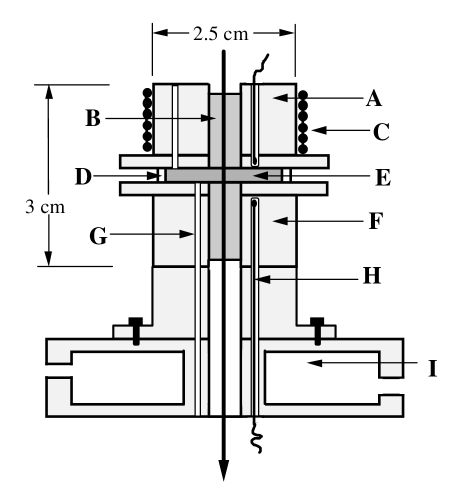
FIG. 1.: Schematic representation of the optical cell for small-angle Rayleigh scattering. A: top plate. B: sapphire windows. C: resistive heater. D: fused quartz ring. E: sample liquid layer. F: bottom plate. G: filling tubes. H: thermistors. I: water circulation chamber.

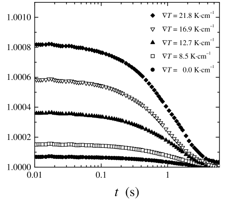
FIG. 2.: Normalized experimental light-scattering correlation functions, obtained at $k=1030$ cm^-1 for a solution of polystyrene ($M_{W}=96,400$, $w=2.50\%$) in toluene subjected to various temperature gradients, $\nabla T$, plotted versus log($t$).

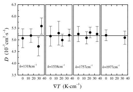
FIG. 3.: Collective mass-diffusion coefficient $D$ of polystyrene ($M_{W}=96,400$, $w=0.50\%$) in toluene deduced from the decay rates of the concentration fluctuations at various values of $k$ and $\nabla T$. The horizontal line represents the average value $D=(5.19\pm 0.04)\times 10^{-7}$ cm² s^-1.

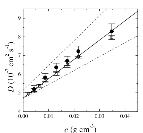
FIG. 4.: Collective mass-diffusion coefficient $D$ as a function of concentration for polystyrene/toluene solutions ($M_{W}=96,400$). $\bullet$: measured in this work by equilibrium and nonequilibrium Rayleigh light scattering. $\Box$: measured by Zhang et al. al. with an optical beam-bending technique[24]. The straight line represents Eq. (16). The dashed lines represent the limits over which the literature values are spread.

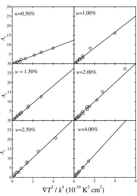
FIG. 5.: The amplitude $A_{c}$ of the nonequilibrium concentration fluctuations in dilute and semidilute polystyrene/toluene solutions ($M_{W}=96,400$) at 25^∘C and at various concentrations as a function of $(\nabla T)^{2}/k^{4}$. The solid lines represent linear fits to the experimental data for each concentration with slope $A_{c}$ given in Table V.

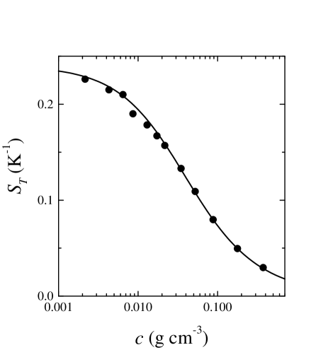
FIG. 6.: Experimental values of the Soret coefficient of polystyrene ($M_{W}=96,400$) in toluene at 25^∘ as a function of polymer concentration $c$. The solid curve represents Eq. (24) with $k_{S}=24$ cm³ g^-1, $S_{T0}=0.24$ K^-1, and $r_{S}$ determined by fitting to be $r_{S}=1.16\pm 0.07$ .

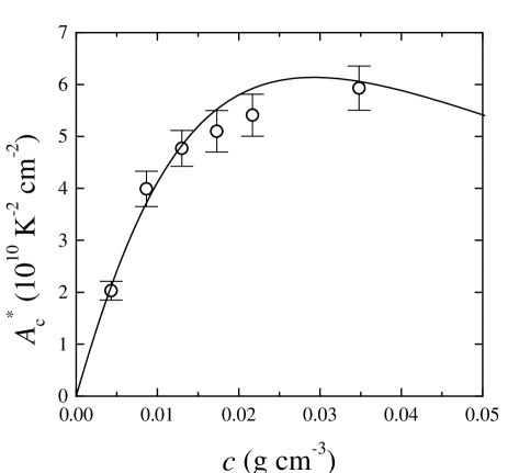
FIG. 7.: Comparison of the measured values of the strength, $A_{c}^{*}$, of the nonequilibrium enhancement of the concentration fluctuations (open circles) with the theoretical values (solid curve) calculated from Eq. (9).

REFERENCES

- [1] J. Berne and S. Pecora, Dynamic Light Scattering (McGraw-Hill, New York, 1980).
- [2] J.P. Boon and S. Yip, Molecular Hydrodynamics (McGraw-Hill, New York, 1980).
- [3] J.R. Dorfman, T.R. Kirkpatrick, and J.V. Sengers, Annu. Rev. Phys. Chem. 45, 213 (1994).
- [4] T.R. Kirkpatrick, E.G.D. Cohen, and J.R. Dorfman, Phys. Rev. Lett. 42, 862 (1979), 44, 472 (1980), Phys. Rev. A 26, 950, 972, 995 (1982).
- [5] D. Ronis and I. Procaccia, Phys. Rev. A 26, 1812 (1982)
- [6] B.M. Law and J.V. Sengers, J. Stat. Phys. 57, 531 (1989).
- [7] R. Schmitz and E.G.D. Cohen, J. Stat. Phys. 39, 285 (1985); 40, 431 (1985).
- [8] G. Grinstein, D.-H. Lee, and S. Sachdev, Phys. Rev. Lett. 64, 1927 (1990).
- [9] P.N. Segrè, R.W. Gammon, J.V. Sengers, and B.M. Law, Phys. Rev. A 45, 714 (1992).
- [10] W.B. Li, P.N. Segrè, R.W. Gammon, and J.V. Sengers, Physica A 204, 399 (1994).
- [11] J.C. Nieuwoudt and B.M. Law, Phys. Rev. A 42, 2003 (1990).
- [12] B.M. Law and J.C. Nieuwoudt, Phys. Rev. A 40, 3880 (1989).
- [13] P.N. Segrè, R. Schmitz, and J.V. Sengers, Physica A 195, 31 (1993).
- [14] P.N. Segrè and J.V. Sengers, Physica A 198, 96 (1993).
- [15] A. Vailati and M. Giglio, Phys. Rev. E 58, 4361 (1998).
- [16] P.C. Hohenberg and J.B. Swift, Phys. Rev. A 46, 4773 (1992)
- [17] H. van Beijeren and E.G.D. Cohen, J. Stat. Phys. 53, 77 (1988).
- [18] I. Pagonabarraga, J.M. Rubí, and L. Torner, Physica A 173, 111 (1991).
- [19] P.N. Segrè, R.W. Gammon, and J.V. Sengers, Phys. Rev. E 47, 1026 (1993).
- [20] W.B. Li, P.N. Segrè, J.V. Sengers, and R.W. Gammon, J. Phys. Condens. Matter 6, A119 (1994).
- [21] A. Vailati and M. Giglio, Phys. Rev. Lett. 77, 1484 (1996); Prog. Colloid. Polym. Sci. 104, 76 (1997).
- [22] W. Köhler and B. Müller, J. Chem. Phys. 103, 4367 (1995).
- [23] K.J. Zhang, M.E. Briggs, R.W. Gammon, and J.V. Sengers, J. Chem. Phys. 104, 6881 (1996).
- [24] K.J. Zhang, M.E. Briggs, J.V. Sengers, R.W. Gammon, and J.F. Douglas, J. Chem. Phys. 111, 2270 (1999).
- [25] W.B. Li, K.J. Zhang, J.V. Sengers, R.W. Gammon, and J.M. Ortiz de Zárate, Phys. Rev. Lett. 81, 5580 (1998).
- [26] M.A. Anisimov, V.A. Agayan, A.A. Povodyrev, J.V. Sengers, and E.E. Gorodetskii, Phys. Rev. E 57, 1946 (1998).
- [27] R. Schmitz, Physica A 206, 25 (1995).
- [28] I. Noda, Y. Higo, N. Ueno, and T. Fujimoto, Macromolecules 17, 1055 (1984).
- [29] Y. Higo, N. Ueno, and I. Noda, Polym. J. 15, 367 (1983).
- [30] B.M. Law, P.N. Segrè, R.W. Gammon, and J.V. Sengers, Phys. Rev. A 41, 816 (1990).
- [31] Th.G. Scholte, J. Polym. Sci. Part A-2 8, 841 (1970).
- [32] P.N. Pusey, J.M. Vaughan, and G. Williams, J. Chem. Soc. Fadaray Trans. 70, 1696 (1970).
- [33] B. Appelt and G. Meyerhoff, Macromolecules 13, 657 (1980).
- [34] V. Petrus, B. Porsch, B. Nyström, and L.- O. Sundelöf, Makromol. Chem. 183, 1279 (1982).
- [35] E. Ozdemir and R.W. Richards, Polymer 24, 1097 (1983).
- [36] M. Ramanathan and M.E. McDonnell, Macromolecules 17, 2093 (1984).
- [37] B.K. Varma, Y. Fujita, M. Takakashi, and T. Nose, J. Polym. Sci. 22, 1781 (1984).
- [38] K. Huber, S. Bantle, P. Lutz and W. Burchard, Macromolecules 18, 1461 (1985).
- [39] B.D. Freeman, D.S. Soane, and M.M. Denn, Macromolecules 23, 245 (1990).
- [40] W. Köhler, C. Rosenauer, and P. Rossmanith, Int. J. Thermophys. 16, 11 (1995).
- [41] P. Vidakovic and F. Rondelez, Macromolecules 18, 700 (1985).
- [42] H. Yamakawa, Modern Theory of Polymer Solutions, (Harper&Row, New York, 1971).
- [43] Y. Takakashi, Y. Isono, I. Noda, and M. Nagasawa, Macromolecules 18, 1002 (1985).
- [44] L.A. Papazian, Polymer 10, 399 (1969).
- [45] F. Brochard and P.G. de Gennes, C.R. Acad. Sc. Paris 293-II, 1025 (1981).
- [46] B. Nyström, and J. Roots, Polymer 33, 1548 (1992).
- [47] The expression for the exponent given in reference [REFERENCES] is given with the wrong sign.
- [48] X.L. Wu, D.J. Pine, P.K. Dixon, Phys. Rev. Lett. 66, 2408 (1991).
- [49] S.T. Milner, Phys. Rev. Lett. 66, 1477 (1991).
- [50] A. Onuki, Phys. Rev. Lett. 62, 2472 (1989).
- [51] A. Vailati and M. Giglio, Nature 390, 262 (1997).