Time Dependent Theory for Random Lasers

The interplay of localization and amplification is an old and interesting topic in physics research[1]. With promising properties, mirror-less random laser systems are widely studied[2, 3, 4, 5, 6] both experimentally and theoretically. Recently new observations [2] of laser-like emission were reported and showed new interesting properties of amplifying media with strong randomness. First, sharp lasing peaks appear when the gain or the length of the system is over a well defined threshold value. Although a drastic spectral narrowing has been previously observed [3], discrete lasing modes were missing. Second, more peaks appear when the gain or the system size further increases over the threshold. Third, the spectra of the lasing system is direction dependent, not isotropic. To fully explain such an unusual behavior of stimulated emission in random systems with gain, we are in need of new theoretical ideas.

Theoretically, a lot of methods have been used to discuss the properties of such random lasing systems. Based on the time-dependent diffusion equation, earlier work of Letokhov [1] predicted the possibility of lasing in a random system and Zyuzin [4] discussed the fluctuation properties near the lasing threshold. Recently, John and Pang [5] studied the random lasing system by combining the electron number equations of energy levels with the diffusion equation. Such a consideration predicted a reduction in the threshold gain for a laser action due to the increased optical path from diffusion. It also verified the narrowing of the output spectrum when approaching the gain threshold. By using the diffusion approach is not possible to explain the lasing peaks observed in the recent experiments[2] in both semiconductor powders and in organic materials. The diffusive description of photon transport in gain media neglects the phase coherence of the wave, so it gives limited information for the wave propagation in the gain media. Another approach which is based on the time-independent wave equations for the random gain media can go beyond the diffusive description [6, 7, 8, 9, 10]. But as was shown recently [11], the time-independent method is only useful in determining the lasing threshold. When the gain or the length of system is larger than the threshold value, the time-independent description will give a totally unphysical picture for such a system. To fully understand the random lasing system, we have to deal with time-dependent wave equations in random systems. On the other hand, the laser physics community [12, 13] has developed some phenomenological theories to deal with gain media which were overlooked by the researchers working on random systems.

In this paper we introduce a model by combining these semi-classical laser theories with Maxwell equations. By incorporating a well-established FDTD ( finite-difference time-domain) [14] method we calculate the wave propagation in random media with gain. Because this model couples electronic number equations at different levels with field equations, the amplification is nonlinear and saturated, so stable state solutions can be obtained after a long relaxation time. The advantages of this FDTD model are obvious, since one can follow the evolution of the electric field and electron numbers inside the system. From the field distribution inside the system, one can clearly distinguish the localized modes from the extended ones. One can also examine the time dependence of the electric field inside and just outside the system. Then after Fourier transformation, the emission spectra and the modes inside the system can be obtained.

Our system is essentially a one-dimensional simplification of the real experiments [2, 3]. It consists of many dielectric layers of real dielectric constant of fixed thickness, sandwiched between two surfaces, with the spacing between the dielectric layers filled with gain media (such as the solution of dye molecules). The distance between the neighboring dielectric layers is assumed to be a random variable. The overall length of the system is $L$.

Our results can be summarized as follows: ($i$) As expected for periodic and $short$ ($L<\xi$, $\xi$ is the localization length) random system, an extended mode dominates the field and the spectra. ($ii$) For either strong disorder or the long ($L\gg\xi$) system, we obtain a low threshold value for lasing. By increasing the length or the gain (higher gain can be achieved by increasing the pumping intensity) more peaks appear in the spectra. By examining the field distribution inside the system, one can clearly see that these lasing peaks are coming from localized modes. ($iii$) When the gain or the pumping intensity increases even further, the number of lasing modes do not increase further, but saturate to a constant value, which is proportional to the length of system for a given randomness. And ($i$v) the emission spectra are not same for different output directions which show that the emission is not isotropic. These findings are in agreement with recent experiments [2] and also make new predictions.

The binary layers of the system are made of dielectric materials with dielectric constant of $\varepsilon_{1}=\varepsilon_{0}$ and $\varepsilon_{2}=4\times\varepsilon_{0}$ respectively. The thickness of the first layer, which simulates the gain medium, is a random variable $a_{n}=a_{0}(1+W\gamma)$ where $a_{0}=300$nm, $W$ is the strength of randomness and $\gamma$ is a random value in the range [-0.5, 0.5]. The thickness of second layer, which simulates the scatterers, is a constant $b=180$nm. In the first layer, there is a four-level electronic material mixed inside. An external mechanism pumps electrons from ground level ($N_{0}$) to third level ($N_{3}$) at certain pumping rate $P_{r}$, which is proportional to the pumping intensity in experiments. After a short lifetime $\tau_{32}$, electrons can non-radiative transfer to the second level ($N_{2}$). The second level ($N_{2}$) and the first level ($N_{1}$) are called the upper and the lower lasing levels. Electrons can be transfered from the upper to the lower level by both spontaneous and stimulated emission. At last, electrons can non-radiative transfer from the first level ($N_{1}$) back to the ground level ($N_{0}$). The lifetimes and energies of upper and lower lasing levels are $\tau_{21}$, $E_{2}$ and $\tau_{10}$, $E_{1}$ respectively. The center frequency of radiation is $\omega_{a}={(E_{2}-E_{1})}/{\hbar}$ which is chosen to be equal to $2\pi\times 6\cdot 10^{14}$ $Hz$ ($\lambda=499.7$ $nm$). Based on real materials [13], the parameters $\tau_{32}$, $\tau_{21}$ and $\tau_{10}$ are chosen to be $1\times 10^{-13}$s, $1\times 10^{-9}$s and $1\times 10^{-11}$s. The total electron density $N_{0}^{0}=N_{0}+N_{1}+N_{2}+N_{3}$ and the pump rate $P_{r}$ are the controlled variables according to the experiments [2].

The time-dependent Maxwell equations are given by $\bf{{\nabla}\times\bf{E}}=-{\partial\bf{B}}/{\partial t}$ and $\bf{{\nabla}\times\bf{H}}=\varepsilon{\partial\bf{E}}/{\partial t}+{\partial\bf{P}}/{\partial t}$, where $\bf{B}=\mu\bf{H}$ and $\bf{P}$ is the electric polarization density from which the amplification or gain can be obtained. Following the single electron case, one can show [13] that the polarization density in the presence of an electric field obeys the following equation of motion:

$$\frac{d^{2}P(t)}{dt^{2}}+\Delta\omega_{a}\frac{dP(t)}{dt}+{\omega_{a}^{2}}P(t)=\frac{\gamma_{r}}{\gamma_{c}}\frac{e^{2}}{m}\Delta N(t)E(t)$$ (1)

where $\Delta\omega_{a}={1}/{\tau_{21}}+{2}/{T_{2}}$ is the full width at half maximum linewidth of the atomic transition. $T_{2}$ is the mean time between dephasing events which is taken to be $2.18\times 10^{-14}$s, $\Delta N(t)=N_{1}-N_{2}$ and $\gamma_{r}={1}/{\tau_{21}}$ is the real decay rate of the second level and $\gamma_{c}=\frac{e^{2}}{m}\frac{{\omega_{a}}^{2}}{6\pi\varepsilon_{0}c^{3}}$ is the classical rate. It is easy to derive [13] from Eq. (1) that the amplification line shape is Lorentzian and homogeneously broadened. Eq. (1) can be thought as a quantum mechanically correct equation for the induced polarization density $P(t)$ in a real atomic system.

The equations giving the number of electrons on every level can be expressed as follows:

$$\frac{dN_{3}(t)}{dt} = P_{r}N_{0}(t)-\frac{N_{3}(t)}{\tau_{32}}$$ (2)

$$\frac{dN_{2}(t)}{dt} = \frac{N_{3}(t)}{\tau_{32}}+\frac{1}{\hbar\omega_{a}}E(t)\frac{dP(t)}{dt}-\frac{N_{2}(t)}{\tau_{21}}$$ (3)

$$\frac{dN_{1}(t)}{dt} = \frac{N_{2}(t)}{\tau_{21}}-\frac{1}{\hbar\omega_{a}}E(t)\frac{dP(t)}{dt}-\frac{N_{1}(t)}{\tau_{10}}$$ (5)

$$\frac{dN_{0}(t)}{dt} = \frac{N_{1}(t)}{\tau_{10}}-P_{r}N_{0}(t)$$ (6)

where $\frac{1}{\hbar\omega}E(t)\frac{dP(t)}{dt}$ is the induced radiation rate from level 2 to level 1 or excitation rate from level 1 to level 2 depending on its sign.

To excite the system, we must introduce sources into the system. To simulate the real laser system, we introduce sources homogeneously distributed in the system to simulate the spontaneous emission. We make sure that the distance between the two sources $L_{s}$ is smaller than the localization length $\xi$. Each source generates waves of a Lorentzian frequency distribution centered around $\omega_{a}$, with its amplitude depending on $N_{2}$. In real lasers, the spontaneous emission is the most fundamental noise [12, 13] but generally submerged in other technical noises which are much larger. In our system, the simulated spontaneous emission is the $only$ noise present, and is treated self-consistently. This is the reason for the small background in the emission spectra shown below.

There are two leads, both with width of 3000 nm, at the right and the left sides of the system and at the end of the leads we use the Liao method [14] to impose an absorbing-boundary conditions (ABC). In the FDTD calculation, discrete time step and space steps are chosen to be $10^{-17}$s and $10^{-9}$m respectively. Based on the previous time steps we can calculate the next time step ($n+1$ step) values. First we obtain the $n+1$ time step of the electric polarization density $P$ by using Eq. (1), then the $n+1$ step of the electric and magnetic fields are obtained by Maxwell’s equations and at last the $n+1$ step of the electron numbers at each level are calculated by Eq. (2). The initial state is that all electrons are on the ground state, so there is no field, no polarization and no spontaneous emission. Then the electrons are pumped and the system begins to evolve according to equations.

We have performed numerical simulations for periodic and random systems. First, for all the systems, a well defined lasing threshold exists. As expected, when the randomness becomes stronger, the threshold intensity decreases because localization effects make the paths of waves propagating inside the gain medium much longer.

For a periodic or $short$ ($L<\xi$) random system, generally only one mode dominates the whole system even if the gain increases far above the threshold. This is due to the fact that the first mode can extend in the whole system, and its strong electric field can force almost all the electrons of the upper level $N_{2}$ to jump down to the $N_{1}$ level quickly by stimulated emission. This leaves very few upper electrons for stimulated emission of the other modes. In other words, all the other modes are suppressed by the first lasing mode even though their threshold values are only a little bit smaller than the first one. This phenomenon also exists in common lasers [12].

For $long$ ($L>>\xi$) random systems, richer behavior is observed. First we find that all the lasing modes are localized and stable around their localization centers after a long time. Each mode has its own specific frequency and corresponds to a peak in the spectrum inside the system. When the gain increases beyond the threshold, the electric field pattern (see Fig. 1a) shows that more localized lasing modes appear in the system and the spectrum inside the system (see Fig. 1b) gives more sharp peaks just as observed in the experiments [2]. This is clearly seen in Figs 1a and 1b for a 80 cell random system, above threshold. In Figs. 1c and 1d similar values are shown for the 160 cell system. Notice that both the number of localized modes (Fig. 1c) of the field, as well the number of lasing peaks (Fig. 1d) are larger now. The exact position of the lasing peaks depends on the random configuration. Notice that the lasing peaks are much narrower than the experimental ones [2]. This is due to the 1d nature of our model. In the present case only two escaping channels exist, so it’s more difficult for the wave to get out from the system which has a higher quality factor. When the gain is really big, we find the number of lasing modes will not increase any more, so a saturated number $N_{m}$ of lasing modes exists for the long random system. This is clearly seen in Fig. 2, where we plot the number of modes $N_{m}$ vs the pumping rate $P_{r}$. In Fig. 3, we plot the spectral intensity vs the wavelength for different input transitions (or equivalently pumping rates). Notice these results are in qualitative agreement with the experimental results shown in Fig. 2 of the paper of Cao et. al. [2].

These multi-lasing peaks and the saturated-mode-number phenomena are due to the interplay between localization and amplification. Localization makes the lasing mode strong around its localization center and exponentially small away from its center so that it only suppress the modes in this area by reducing $N_{2}$. When a mode lases, only those modes which are $far$ $enough$ from this mode can lase afterwards. So more than one mode can appear for a long system and each mode seems to $repel$ each other. Because every lasing mode dominates a certain area and is separated from other modes, only a limited number of lasing modes can exist for a finite long system even in the case of large amplification. We therefore expect that the number of surviving lasing modes $N_{m}$ should be proportional to the length of the system $L$ when the amplification is very large. Since the ”mode-repulsion” property is coming from the localization of the modes we expect that the average mode length $L_{m}=L/N_{m}$ should be proportional to localization length $\xi$ too. In Fig.4, we plot $N_{m}$ vs the length of the systems $L$ when we increase the length from 80 cells to 320 cells and keep all other parameters the same. In Fig.4, we also plot the average mode length $L_{m}$ vs the localization length $\xi$ when we change the random strength W for a 320 cell system. The localization lengths are calculated using the transfer-matrix method by averaging 10,000 random configurations. These results confirm that indeed $N_{m}\propto L$ and $L_{m}\propto\xi$. It will be very interesting if these predictions can be checked experimentally.

The emission spectra at the right and left side of the system are quite different. This can be explained from the field patterns shown in Fig. 1a and Fig. 1c. Notice the localized modes are not similar at both sides of the system. This is the reason for this difference in the output spectrum. In Fig. 1d we denote with $l$ and $r$ the output modes from the left and the right side of our 1d system, respectively. The non-isotropic output spectra of real $3D$ experiments [2] might be explained by assuming that every localized mode has its intrinsic direction, strength and position, and the detected output spectra in experiments at different directions are the overlap of contributions from many modes. So generally they should be different. Most of the modes are not able to escape in our model and this is because of the 1D localization effects and exchange of energy between modes.

In summary, by using a FDTD method we constructed a random four-level lasing model to study the interplay of localization and amplification. Unlike the time-independent models, the present formulation calculates the field evolution beyond the threshold amplification. This model allows us to obtain the field pattern and spectra of localized lasing modes inside the system. For random systems, we can explain the multi-peaks and the non-isotropic properties in the emission spectra, seen experimentally. Our numerical results predict the ”mode-repulsion” property, the lasing-mode saturated number and average modelength. We also observed the exchange of energy between the localized modes which is much different from common lasers and this is essential for further research of mode competition and evolution in random laser. All of these properties are from the interplay of the localization and amplification where new physics phenomena can be found.

Ames Laboratory is operated for the U.S. Department of Energy by Iowa State University under Contract No. W-7405-Eng-82. This work was supported by the director for Energy Research, Office of Basic Energy Sciences.

FIG. 1.: (a) The amplitude of the electric field $A_{E}$ vs the length of the system and (b) the spectra intensity $I_{e}$ vs the wavelength for a 80 cell system with $W=1.2$, ${N_{0}}^{0}=5.5\times 6.02\times 10^{23}/m^{3}$ and $P_{r}=1\times 10^{10}$$s^{-1}$. In (c) and (d) $A_{E}$ and $I_{e}$ for a 160 cell system.

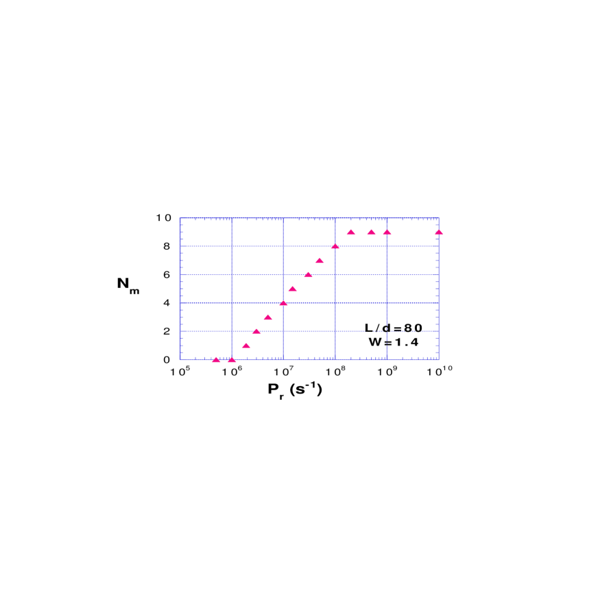
FIG. 2.: The number of modes $N_{m}$ versus the pumping rate $P_{r}$, for a 80 cell system with W=1.4. The critical pumping rate $P_{r}^{c}$=$10^{6}s^{-1}$

.

FIG. 3.: The spectral intensity vs the wavelength for the 80 cell system with W=1.4 for different pumping rates $P_{r}$. $P_{r}$ in units of $s^{-1}$ is (a) $10^{4}$, (b) $10^{6}$, (c) $10^{7}$ and (d) $10^{10}$

.

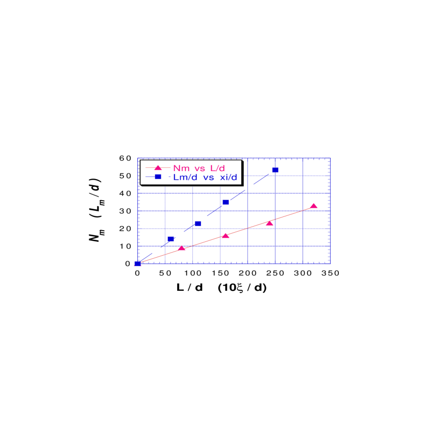
FIG. 4.: The number of modes $N_{m}$ vs the length of the system $L/d$, where d=$<a_{n}>$+b=480 nm is the size of the cell. Also the average mode length $L_{m}/d$ vs the localization length $10\times\xi/d$ for different disorder strength W for a 320 cell system. The rest of the parameters are the same as the ones of Fig. 1.

REFERENCES

- [1] V. S. Letokhov, Sov. Phys. JEPT 26, 835 (1968).
- [2] H. Cao, Y. G. Zhao, S. T. Ho, E .W. Seelig, Q. H. Wang, and R. P .H .Chang, Phys. Rev. Lett. 82, 2278 (1999); S. V. Frolov, Z. V. Vardeny, K. Yoshino, A. Zakhidov and R. H. Baughman, Phys. Rev. B 59, 5284 (1999)
- [3] N. M. Lawandy, R. M. Balachandran, S. S. Gomers, and E. Sauvain, Nature 368, 436 (1994); D. S. Wiersma, M. P. van Albada and Ad Lagendijk, Phys. Rev. Lett. 75, 1739 (1995).
- [4] A. Yu. Zyuzin, Phys. Rev. E 51, 5274 (1995)
- [5] S. John and G. Pang, Phys. Rev. A 54, 3642 (1996), and references therein.
- [6] Qiming Li, K. M. Ho, and C. M. Soukoulis, unpublished.
- [7] P. Pradhan, N. Kumar, Phys. Rev. B 50, 9644 (1994).
- [8] Z. Q. Zhang, Phys. Rev. B 52, 7960 (1995).
- [9] J. C. J. Paasschens, T. Sh. Misirpashaev and C. W. J. Beenakker, Phys. Rev. B 54, 11887 (1996).
- [10] Xunya Jiang, C. M. Soukoulis, Phys. Rev. B. 59, 6159 (1999).
- [11] Xunya Jiang, Qiming Li, C. M. Soukoulis, Phys. Rev. B. 59 9007
- [12] M. Sargent III, M. O. Scully, and W. E. Lamb. Jr, Laser Physics (Addison-Wesley, Reading, Mass., 1974).
- [13] Anthony E. Siegman, Lasers (Mill Valley, California, 1986)
- [14] A. Taflove, Computational Electrodynamics (Artech House, London, 1995).
.
.