Numerical studies of domains and bubbles of Langmuir monolayers

Abstract

A numerical algorithm based on the finite element methods has been developed to accurately determine the shape of the boundary of a domain containing “boojum” textures. Within the context of the simple model we adopt, the effects of both bulk elastic anisotropy and line-tension anisotropy on the domain boundary can be examined. It is found that line-tension anisotropy must be present in order to account for domains with protruding features. Both elastic anisotropy and anisotropic line-tension can result in domains with indentations. The numerical algorithm has been extended to investigate the problem of a bubble in extended region ordered phase.

I Introduction

A Langmuir monolayer is a single molecular layer of insoluble surfactant molecules spread on the air/water interface. The surfactants are typically amphiphilic molecules with a hydrophilic headgroup and a hydrophobic tail. Each of the individual molecules has internal degrees of freedom, namely the tilt and the tilt azimuth. Such a system exhibits complex phase structure[1]. The “tilted” phases have uniform tilt and possess mesoscopic ordering in the tilt azimuth. The structure of the tilt azimuth is typically observed as a variation in the light intensity under a polarized light microscope. The tilt azimuth organization is referred to as the texture. Various classes of the texture have been observed, such as the stripes in the bulk[2], the star configuration[3, 4] and “boojums”[5] in the domains of the tilted phase, when it coexists with an isotropic phase. The term Boojum refers to a class of textures that has a tilt azimuth distribution which resembles the structure of the orbital angular momentum in a superfluid ³He droplet[6]. The “boojum” texture, in which the tilt azimuth is distributed continuously without singularity, will be the subject of this report. Domains observed to contain a boojum texture are not circular in shape[5, 7]. In addition, micron-size bubbles, which are regions of isotropic phase surrounded by a “tilted” phase, have been found to have non-circular shapes [7]. The local tilt azimuth in the “tilted” phase around the bubble exhibits a non-trivial structure, which has been termed an “inverse boojum”. The relationship between experimentally observed textures and the underlying structure of the ordered phase has attracted attention in the literature recently. In particular, the “boojum” texture was first discussed by Mermin in the context of orbital angular momental distribution in superfluid ³He droplet [6]. Similar texture of has been found and discussed in the liquid crystal films[8, 9]. An extensive discussion on the various classes of textures in the Langmuir monolayers can be found in Ref. [4].

The problem of the equilibrium shape of, and the texture contained in domains in a Langmuir monolayer has been investigated by Rudnick and Bruinsma [10] who varied both the texture and the boundary analytically in a perturbative manner. It was discovered that a non-circular boundary represents the equilibrium shape of a domain only when there is bulk or line-tension anisotropy[5, 10]. The equilibrium domain boundary was derived as a function of line-tension anisotropy. Galatola and Fournier [11] obtained numerically, in a fixed background texture, the equilibrium boundary when both elastic and line-tension anisotropies are present. Rivière and Meunier [5] have attempted to explain the observed non-circular domains in terms of elastic anisotropy. Evidence of bubbles with a non-circular boundary and an “inverse boojum” has been reported, and a qualitative theoretical discussion of the equilibrium shape and texture associated with the bubbles can be found in Ref. [7]. In the spirit of Ref. [10], the authors have analyzed in Ref. [12] the equilibrium texture and boundary shape combinations perturbatively to the first order in both the bulk elastic and line-tension anisotropies. The approach describes the infinitesimal response of the texture and the boundary to anisotropic parameters. However, when the correction is large enough to be observed, the validity of first order perturbative calculations becomes questionable. The extension of the perturbative approach to include higher order corrections is algebraically formidable. If one is to go beyond first order effects, the use of numerical techniques in this problem is inevitable.

The major challenges in this problem are, first, the evaluation of a 2D texture with a boundary condition on the boundary, which is, itself, variable. Secondly, not only must the texture be evaluated with high accuracy, but a precise determinations of the derivatives of the texture on the boundary is also crucial to the computation of the boundary shape. The authors have developed a numerical algorithm based on the finite element method (FEM) with adaptive mesh refinement [13] for the evaluation of a 2D texture and its derivatives. The boundary corrections can then be computed using the Runge-Kutta methods[14]. Implementation of the numerical method reveals various classes of domain shapes ranging from those with indentations to those with protruding features and, additionally, of cigar-shaped domains. The effects of bulk elastic anisotropy have also been examined. These studies lead us to the conclusion that, as least for those domain shapes observed to date, it is more likely that the line-tension anisotropy is responsible for non-circular domains. A brief account of the study described above has appeared in an earlier publication[15]. The numerical results also confirm that the qualitative conclusion to be drawn from the perturbative treatment are preserved up to large anisotropic parameter.

In this report, we describe in detail the implementation of the numerical methods that lead us to the results reported in Ref [15]. The extension of the algorithm to allow for computation in the case of bubble has also been examined. It is verified numerically that bubbles acquire a non-trivial boundary shape when only the first term in the Fourier expansion of the line tension is present. This result contrasts with what is known to be true in the case of domain, which remains circular in the presence of this low-order line-tension anisotropy[10]. With the use of our numerical algorithm, we are able to examine the effects of the bulk elastic anisotropy on the shape of the bubble and on the texture that surrounds it. We find that bulk elastic anisotropy significantly affects the texture in the condensed phase around the bubble while leaving the boundary nearly unmodified.

The organization of this paper is as follows. Section II contains the details of the computational scheme for the evaluation of the equilibrium textural and boundary configuration for domains. The discussion covers the derivation of the simplest variational formulation of the finite element method in our specific application, the Runge-Kutta method and the combined algorithm. In Sec. III, results for the domain are examined. Section IV describes the extension of the numerical algorithm to the problem of bubbles. An examination of the results of the perturbative treatment follows. New results on the effect of the bulk elastic anisotropy on the textures around the bubbles are discussed. Finally, Sec. V contains concluding remarks and discusses possible future extensions of the numerical methods discussed in this report.

II The Numerical Algorithm

The model that we adopt for the Langmuir monolayer is a simple elastic model of an ordered media associated with $XY$-like order parameter—a 2 dimensional unit vector $\hat{c}(x,y)$, which can be parameterized as $\hat{x}\cos\Theta(x,y)+\hat{y}\sin\Theta(x,y)$  [12]. The quantities $\hat{x}$ and $\hat{y}$ are unit vectors in a Cartesian coordinate system, and $\Theta(x,y)$ is the angle between $\hat{c}$ and the x-axis. The energy of the system contains contributions from the boundary, $\Gamma$, in addition to the bulk, $\Omega$. The most general form of the elastic energy[4, 8] for such a system with in-plane reflection symmetry (an achiral system) can be written as

$$H[\Theta]=\int_{\Omega}{\cal H}_{b}dA+\oint_{\Gamma}\sigma(\vartheta-\Theta)ds,$$ (1)

where

$${\cal H}_{b} = \frac{K_{s}}{2}|\nabla\cdot\hat{c}|^{2}+\frac{K_{b}}{2}|\nabla\times\hat{c}|^{2},$$ (2)

$$\sigma(\phi) = \sigma_{0}+\sum_{n=1}a_{n}\cos n\phi,$$ (3)

$K_{s}$, $K_{b}$ are respectively the splay and bend elastic moduli, and $\vartheta$ is the angle between the outward normal $\hat{n}$ of $\Gamma$ and the x-axis. The setup of the computations is shown in Fig. 1. In terms of the average Frank modulus $\kappa$ and the coefficient of elastic anisotropy, $b$ where $2\kappa\equiv K_{b}+K_{s}$ and $2\kappa b\equiv K_{s}-K_{b}$, the extrema of the elastic energy Eq. (1) occurs when $\Theta(x,y)$ and the bounding curve $\Gamma$ satisfy their respective equilibrium conditions. The extremum equations for $\Theta(x,y)$ are

$$-\nabla^{2}\Theta+b\left[\left(\Theta_{xx}-\Theta_{yy}\right)\cos 2\Theta+2\Theta_{xy}\sin 2\Theta\right.$$ (4)

$$\left.+\left(-\Theta_{x}^{2}+\Theta_{y}^{2}\right)\sin 2\Theta+2\Theta_{x}\Theta_{y}\cos 2\Theta\right] =0,$$ (5)

in $\Omega$ and

$$\kappa\Theta_{n}\left[1-b\cos 2(\vartheta-\Theta)\right]+$$ (6)

$$\kappa b\Theta_{t}\sin 2(\vartheta-\Theta)-\sigma^{\prime}(\vartheta-\Theta) =0,$$ (7)

along $\Gamma$, where $\Theta_{n}=\hat{n}\cdot\nabla\Theta$, $\Theta_{t}=\hat{t}\cdot\nabla\Theta$, $\hat{t}$ being the tangential vector. The extremum equation for the bounding curve $\Gamma$, in terms of $\Theta_{n}$, $\Theta_{t}$ and $d\vartheta/ds$, is

$${\cal H}_{b}-\sigma^{\prime}(\vartheta-\Theta)\Theta_{n}-\sigma^{\prime\prime}(\vartheta-\Theta)\Theta_{t}$$ (8)

$$+\left[\sigma(\vartheta-\Theta)+\sigma^{\prime\prime}(\vartheta-\Theta)\right]\frac{d\vartheta}{ds}+\lambda =0,$$ (9)

where $ds$ is the length element of $\Gamma$ traversing in the positive direction of $\Omega$ and $\lambda$ is a Lagrange multiplier that enforces the condition of constant enclosed area.

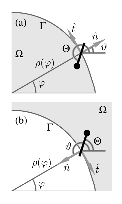
FIG. 1.: The geometry of the calculations for (a) domains and (b) bubbles in plane-polar coordinates where the boundary $\Gamma$ is parameterized by $\rho(\varphi)$. The gray area is the bulk designated by $\Omega$. $\hat{n}$ and $\hat{t}$ are the outward normal and the tangent, respectively. $\Theta$ is the angle between the $\hat{c}$-director and the x-axis and $\vartheta$ is the angle between the outward normal of the boundary and the x-axis.

The equations for both $\Theta$ and $\Gamma$ are complex and highly non-linear. Closed form analytic solution of the extremum equations is almost impossible. Attempts have been made to solve the simultaneous equation perturbatively to first order in the elastic and line-tension anistropies [12]. When the corrections to the boundaries are large enough to be observable, it is not expected that the results are accurate and high order corrections have to be taken into account. However, these attempts provide us with insight with regard to the infinitesimal response of the boundary to the anisotropies under investigation. In the work to be described below, we analyze the equations numerically in order to further explore the implications of the simple model Eq. (1) for a larger range of the anisotropic parameters. We retain coefficients up to $a_{2}$ in the expansion of the line tension in our analysis, i.e. $\sigma(\phi)=\sigma_{0}+a_{1}(\cos\phi+\gamma\cos 2\phi)$, where the quantity $\gamma\equiv a_{2}/a_{1}$ is defined for convenience. We remark that the analysis will be based on the exact “boojum” texture with circular domain when $\gamma=b=0$. The boundary will be computed in terms of the corrections to the circular boundary. The discussions will be restricted to those domains with boundaries $\Gamma$ for which the distance from each points on the curves to the origin $\mbox{e}^{k(\varphi)}$ is a single-valued function of the polar angle $\varphi$.

The numerical algorithm consists of two parts: in the first part, one evaluates the texture $\Theta$ using an assumed boundary $\Gamma$, and, in the second part, one computes $\Gamma$ using a fixed $\Theta$. Simultaneous equilibrium conditions for $\Gamma$ and $\Theta$ are achieved when a set of predefined self-consistent criteria is met. It is evident from the form of Eq. (9) that accurate determinations of $\Theta$ and its derivatives are the key factors in the solution of the problem. The requirement that the assumed $\Gamma$ in the first part of the algorithm be an arbitrary curve rules out finite difference methods, and militates in favor of finite element methods (FEM). A key feature of the FEM is flexibility in the choice the set of points at which the functional values are to be evaluated, including those on the boundary of the region of interest. This feature is exactly what is needed in our problem, because of the non-trivial geometry of the boundary. One of the simplest constructions of the FEM in 2 dimension is described as follows[13]. We first approximate $\Gamma$ by a polygonal curve, then subdivide $\Omega$ into a set of non-overlapping triangles. No vertex of one triangle lies on the edge of another in the set. The edges of the set of triangle forms a mesh that covers $\Omega$. The process of creating this set of triangles is called mesh generation. The resulting set of triangles is referred to as the triangulation of $\Omega$. Functions are defined by their values on the vertices of the triangles in the triangulation. The value of a function within a triangle is obtained by interpolation using the values on the vertices. Integration over $\Omega$ is the sum of integrations over the triangles which can generally be trivially evaluated. We have now projected our problem, originally on an infinite dimensional space onto a N dimensional space, where N is the number of vertices in the triangulation of $\Omega$. We may write ${\bf\Theta}\equiv(\Theta_{i})$, $i=1,\cdots,{\mbox{N}}$ and

$$\Theta(x,y)=\sum_{i=1}^{N}\Theta_{i}\varphi_{i}(x,y),$$ (10)

where $\varphi_{i}(x,y)$ is a set of basis functions of the N dimensional space. These $\varphi_{i}$’s should not be confused with the polar angle which is denoted by the symbol $\varphi$ without a subscript. The discrete version of the elastic energy functional Eq. (1) is a function of N variables $\Theta_{i}$ and it can be rewritten in terms of $\kappa$ and $b$ as

$$H({\bf\Theta}) = \frac{\kappa}{2}\int_{\Omega}\left\{|\nabla\Theta|^{2}+b\left[\left(-\Theta_{x}^{2}+\Theta_{y}^{2}\right)\cos 2\Theta-\right.\right.$$ (12)

$$\left.\left.2\Theta_{x}\Theta_{y}\sin 2\Theta\right]\right\}\;dA+\oint_{\Gamma}\sigma(\vartheta-\Theta)\;ds,$$

where $\Theta_{x}=\sum\Theta_{i}\varphi_{ix}$, $\Theta_{y}=\sum\Theta_{i}\varphi_{iy}$, $\varphi_{ix}\equiv\partial\varphi_{i}/\partial x$ and $\varphi_{iy}\equiv\partial\varphi_{i}/\partial y$. The equilibrium condition becomes

$$\frac{\partial H({\bf\Theta})}{\partial\Theta_{i}}=0,\;\;\;i=1,\cdots,{\mbox{N}},$$ (13)

which is a discretized version of Eqs. (5) and (7). The set of above equations is not linear. However, if we write them in the form of ${\bf A(\Theta)}\cdot{\bf\Theta}={\bf b(\Theta)}$ where ${\bf A(\Theta)}$ is an ${\mbox{N}}\times{\mbox{N}}$ matrix, ${\bf b(\Theta)}$ and ${\bf\Theta}$ are $1\times{\mbox{N}}$ column matrix as shown below,

$$A_{ij}({\bf\Theta}) = \kappa\int_{\Omega}[\varphi_{ix}\varphi_{jx}(1-b\cos 2\Theta)+$$ (16)

$$\varphi_{iy}\varphi_{jy}(1+b\cos 2\Theta)+$$

$$b(\varphi_{ix}\varphi_{jy}+\varphi_{iy}\varphi_{jx})\sin 2\Theta]dA$$

$$b_{i}(\bf\Theta) = \kappa b\int_{\Omega}[(-\Theta_{x}^{2}+\Theta_{y}^{2})\sin 2\Theta+$$ (19)

$$2\Theta_{x}\Theta_{y}\cos 2\Theta]\varphi_{i}dA+$$

$$\oint_{\Gamma}\sigma^{\prime}(\vartheta-\Theta)\varphi_{i}ds$$

we are able to solve for ${\bf\Theta}$ iteratively using a standard numerical algorithm for the solution of systems of linear equations. We have adopted the method of LU decomposition [14] for solving ${\bf\Theta}$.

The mesh generation algorithm plays an important role in the efficiency of the FEM. An adaptive mesh generation algorithm is used in our program to determine ${\bf\Theta}$. We start with a mesh that is nearly regular throughout $\Omega$ with a predefined grid size. After obtaining a first estimate of ${\bf\Theta}$, a refined mesh is generated. The refined mesh has variable grid sizes over $\Omega$ depending on the variation of ${\bf\Theta}$. Figure 2 depicts the process of mesh generation with adaptive refinement. We are able to determine not only ${\bf\Theta}$, but also the derivatives $\Theta_{t}$ and $\Theta_{n}$, which are necessary for the evaluation the bounding curve, accurately and efficiently with the adaptive mesh generation algorithm.

The next part of the algorithm is the determination of the bounding curve $\Gamma$. We assume the order parameter field $\Theta$ is fixed in Eq. (9) so as to simplify the problem. We then pick an origin in $\Omega$ and parameterize the bounding curve $\Gamma$ as $k(\varphi)$, where $e^{k(\varphi)}\equiv|{\bf r}|$ is the distance between the origin and $(x,y)$ on $\Gamma$, and $\varphi$ is the polar angle. In this parameterization, Eq. (9) is a second order non-linear differential equation in $k(\varphi)$. If we rewrite Eq. (9) as

$$k^{\prime\prime}+q(\varphi;k,k^{\prime})k^{\prime}=r(\varphi;k,k^{\prime})$$ (20)

where $k^{\prime}\equiv dk/d\varphi$ and

$$q(\varphi;k,k^{\prime}) = -\frac{\sigma^{\prime}\Theta_{\varphi}-\sigma^{\prime\prime}\Theta_{k}}{\sigma+\sigma^{\prime\prime}}(1+k^{\prime 2}),$$ (21)

$$r(\varphi;k,k^{\prime}) = \left[1-\frac{\sigma^{\prime}\Theta_{k}+\sigma^{\prime\prime}\Theta_{\varphi}}{\sigma+\sigma^{\prime\prime}}\right](1+k^{\prime 2})+$$ (23)

$$\frac{{\mbox{e}}^{k}{\cal H}_{b}+\lambda}{\sigma+\sigma^{\prime\prime}}(1+k^{\prime 2})^{3/2}.$$

Again, it is possible to integrate the equation for $k(\varphi)$ iteratively using standard method for the solution of ordinary differential equation. The Runge-Kutta method [14] is chosen for our application.

The problem of solving Eqs. (5), (7) and (9) for $\Theta(x,y)$ and $\Gamma$ is reformulated in terms of the solution of Eqs. (13) and (20) iteratively for ${\bf\Theta}$ and $\Gamma$. We begin by assuming an initial boundary $\Gamma^{(0)}$ and texture ${\bf\Theta}^{(0)}$, from which the texture ${\bf\Theta}^{\prime(1)}$ can be computed using FEM. Then iterated texture ${\bf\Theta}^{(1)}={\bf\Theta}^{(0)}+({\bf\Theta}^{\prime(1)}-{\bf\Theta}^{(0)})/\nu_{T}^{(0)}$ is in turn used to evaluate a new accepted boundary $\Gamma^{(1)}=\Gamma^{(0)}+(\Gamma^{\prime(1)}-\Gamma^{(0)})/\nu_{B}^{(0)}$, where $\Gamma^{\prime(1)}$ is obtained using the Runge-Kutta ordinary differential equation integrator on Eq. (9). The process is repeated until both $\Delta{\bf\Theta}^{(n)}\equiv|{\bf\Theta}^{(n)}-{\bf\Theta}^{(n-1)}|$ and $\Delta\Gamma^{(n)}\equiv|\Gamma^{(n)}-\Gamma^{(n-1)}|$ are less then a preset tolerance of the order $O(10^{-5})$. The factors $\nu_{T}^{(n)}$ and $\nu_{B}^{(n)}$ with initial magnitude in the order of $O(10)$ is introduced to avoid numerical instability in these iterative processes. These factors, $\nu^{(n)}_{T}$ and $\nu^{(n)}_{B}$, are adjusted depending on $\Delta{\bf\Theta}^{(n)}$

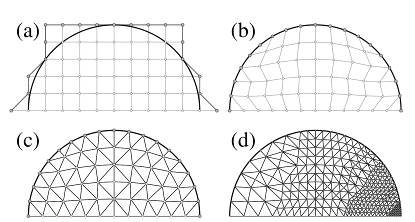
FIG. 2.: The progressive steps towards mesh generation of the problem for the domain, (a) initial choice of grid points in a square lattice, (b) deforming to grid points into the region of interest $\Omega$ and the bounding curve $\Gamma$ while keeping the square lattice topology and connectivity, (c) triangulation using the square lattice connectivity and (d) resulting mesh after adaptive mesh refinement.

and $\Delta\Gamma^{(n)}$, and at the final iterations take on values close to unity.

III Domains

It is well established that the boundary is strictly circular for a domain with a boojum texture when elastic anisotropy and line-tension anisotropy are not present, or $\gamma=b=0$ [10]. This texture-boundary combination is indeed a local minimum of Eq. (1)[16]. Thus, in order for there to be non-circular domains, it is necessary to retain terms in the expansion Eq. (3) up to at least terms going as $a_{2}$. Using the numerical algorithm described above, we have performed systematic studies of the domain textures and shapes in terms of the elastic anisotropy, the line-tension anisotropy as well as the domain size. Before we describe our observation, we note that when $\gamma=b=0$, the exact result is given by a circular boundary of radius $R_{0}$ together with a “boojum” texture with a $+2$ defect located a distance $R_{B}\equiv R_{0}\left(1+\sqrt{1+\rho_{0}^{2}}\right)/\rho_{0}$ from the center of the domain, where $\rho_{0}\equiv R_{0}a_{1}/\kappa$ is the normalized domain radius [10]. An exact equilibrium texture-boundary combination is shown in Fig. 3. The simulated image obtained using the Brewster angle microscopy (BAM) is also displayed in the background. The signature of a “boojum” in a BAM image is a set of straight constant-intensity lines emerging from a virtual defect slightly outside the domain. The light intensity in a BAM image depends on the exact experimental setup and the properties of the monolayer [17]. In the case of all simulated BAM images presented in Fig. 3 and elsewhere in this report, the Brewster angle is taken to be that of water $\Theta_{B}=53.12^{\circ}$, the angle of the analyzer $\alpha$ is equal to $90^{\circ}$, the thickness of the monolayer is assumed to be $d=0.3nm$, the tilt $\Psi$ is $30^{\circ}$, the dielectric constants of the monolayer are $\epsilon_{\perp}=2.31$, $\epsilon_{\parallel}=2.53$ and it is assumed that the wavelength of the light $\lambda=514nm$.

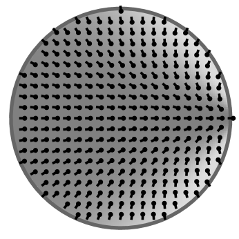
FIG. 3.: Circular domain with a “boojum” texture, $R_{0}=5$, $\sigma_{0}=4$, $a_{1}=1.6$, $a_{2}=0$, $\kappa=1$ and $b=0$. Also shown on the background is the simulated image that would be obtained by Brewster angle microscopy.

We first concentrate on the effects of $b$ and keep $\gamma=0$. When $b<0$, the texture is altered in such a way that the virtual defect appears to move closer to the boundary. This is observed as accelerated convergence of the constant-intensity lines to a point on the boundary. On the other hand, when $b>0$, the texture relaxes as if the virtual defect has moved away from the boundary. The deviation of the texture from the boojum texture is as large as $20\%$ when $|b|\approx 0.8$. The textural response is qualitatively in accord with that reported in Ref. [11]. Although there are significant textural corrections due to the presence of bulk elastic anisotropy, the resultant textures very much resemble a “boojum” as seen in a BAM image as shown in Fig. 4. This means that it is difficult to identify elastic anisotropy based on observation of the textures in the domains. The response of the boundary to elastic anisotropy that we obtain contrasts to that reported in Ref. [11]. The domain acquires an indentation when $b<0$. The indentation remains observable for a large range of domain sizes. The boundary protrudes slightly for $b>0$, as depicted in Fig. 4. The protrusion when $b=+0.8$ is subtle and does not resemble the sharp feature observed experimentally. Thus, elastic anisotropy alone is not capable of accounting for the shapes of the domains observed experimentally. Figure 5 shows domains of various sizes when (a) $b=-0.8$ and (b) $b=+0.8$.

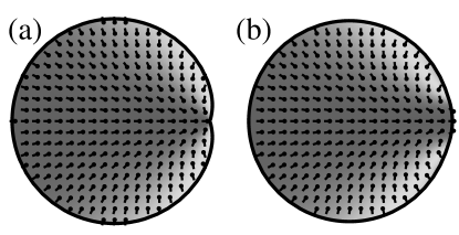
FIG. 4.: The textures and the shapes of domains with $R_{0}=5$, $\sigma_{0}=4$, $a_{1}=1.6$ and $a_{2}=0$. Their stiffness coefficients are (a)$\beta=-0.8$, (b)$\beta=0.8$.

FIG. 5.: The domain shapes computed for $a_{0}=4$, $a_{1}=1.6$ and $a_{2}=0$, and $R_{0}=0.5$, $1$, $2$, $4$, $8$. Their stiffness coefficients are (a)$\beta=-0.8$, (b)$\beta=0.8$. For ease of observation, domains are not shown to scale.

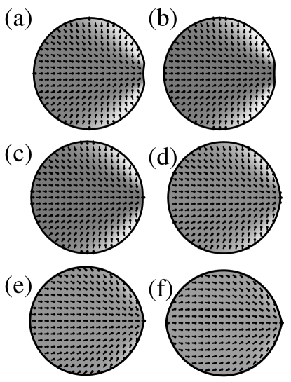
FIG. 6.: The textures and shapes of domains computed for $-0.5<a_{2}<0.5$, $R_{0}=5$, $\sigma_{0}=4$, $a_{1}=1$. (a)$a_{2}=-0.5$, (b)$a_{2}=-0.3$, (c) $a_{2}=-0.1$,( d) $a_{2}=0.1$,(e) $a_{2}=0.3$ and (f) $a_{2}=0.5$.

We now proceed to discuss the role of the line-tension anisotropy, parameterized by $\gamma$, in the textures and the boundaries of the domains. Elastic anisotropy will be eliminated ($b=0$) for simplicity. We first investigate situations when $|\gamma|\leq 1$. For very small domains where $R_{0}a_{1}/\kappa\ll 1$, the texture is almost constant and the dominant contribution to the boundary deformation comes from the $a_{2}$ contribution. The domain is elongated at both ends along the axis connecting its center and the virtual defect when $\gamma>0$ and is flattened at both ends along the same axis when $\gamma<0$. Domain shapes exhibit a 2-fold symmetry. When $R_{0}a_{1}/\kappa\geq 1$, the texture closely resembles the boojum texture and contributes significantly to the boundary distortion through the influence of $\gamma$ in the line-tension. The domain nolonger displays 2-fold symmetry and acquires a protrusion when $\gamma>0$, or an indentation when $\gamma<0$. Figure 6 shows domains of with $\gamma$ ranging from $-0.5$ to $0.5$. The numerical algorithm also allows us to examine domain shape and texture when $a_{1}=0$ and $a_{2}=1$. In this case, the domain acquires a “cigar-shape” and the texture is associated with two virtual $+1$ defects [10, 12]. The progressive changes of the texture and the shape from a system with $a_{1}=1$ and $a_{2}=0$ to one for which $a_{1}=0$ and $a_{2}=1$ are shown in Fig. 7. When both $a_{1}$ and $a_{2}$ are nonzero, the texture can be thought of a superposition of pure $a_{1}$ and pure $a_{2}$ textures. Typically at $R_{0}a_{1}/\kappa\sim 1$, the effect of the set of two $+1$ defects become observable when $\gamma=1/4$. Domains with indentation, protrusions, and the “cigar-shaped” domains, have all been observed experimentally [18].

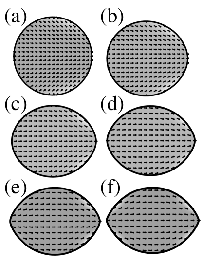
FIG. 7.: The textures and the shapes of domains with $\rho=1$ and $a_{0}=4$. Their coefficients of the anisotropy line tensions are (a)$a_{1}=1$, $a_{2}=0$, (b)$a_{1}=0.8$, $a_{2}=0.2$,(c)$a_{1}=0.6$, $a_{2}=0.4$,(d)$a_{1}=0.4$, $a_{2}=0.6$,(e)$a_{1}=0.2$, $a_{2}=0.8$ and (f)$a_{1}=0$, $a_{2}=1$.

We have already briefly discussed the issue of size dependence in the previous paragraph. To look into this matter in detail, we will examine the particular set of data reported in Ref. [7] in which the domains investigated possess protruding features sharp enough that “excluded angles”, $\Psi_{0}$, characterizing the boundaries can be identified. The definition of $\Psi_{0}$ and the experimental data are depicted in Fig. 8. The key features of this set of experimental data are: (1) $\Psi_{0}$ goes through a maximum as $R_{0}$ varies; (2) there is an abrupt onset of $\Psi_{0}$ in the small $R_{0}$ region; and (3) the intercept at the $\Psi_{0}$-axis when the curve is extrapolated implies $\displaystyle{\lim_{R_{0}\rightarrow\infty}\Psi_{0}\neq 0}$.

Before we make comparisons between theoretical results and the experimental data, we comment on the extraction of $\Psi_{0}$ from computed domain boundaries. It has been shown that within the parameter regime of our discussions, the domain boundaries are smooth and continuous. There is no cusp-like singularity on the boundary. This can be seen in the domains of various sizes shown in Fig. 9. Nevertheless, $\Psi_{0}$ can be unambiguously measured for some of these domains. The values of the parameters utilized here are $\kappa=1$, $\delta=0.4$ and $\gamma=0.5$. To determine $\Psi_{0}$ for these domains, we adopt a systematic scheme that utilizes the function $I\equiv I_{0}\mbox{exp}[-(d^{2}x/dy^{2})^{2}]$ to capture the most likely $\Psi_{0}$ for a given domain bounding curve devised in Ref. [12], where $x(y)$ parameterizes $\Gamma$ in Cartesian coordinates system. Density plots of $I$ as a function of $\Psi\equiv-2\tan^{-1}dx/dy$ and $R_{0}$ for numerical and the perturbative results are shown, respectively, in Figs. 10(a) and (c), the darker regions representing larger $I$, and highlighting the more likely values of $\Psi_{0}$. With the use of this method for the determination of $\Psi_{0}$, we have obtained reasonable agreement between the perturbative analysis and the numerical computations in the large-$R_{0}$ regime. We note here that the value at which $\gamma$ is set, 0.5, is too large for perturbative results to be dependable. However, the perturbative results resemble those obtained numerically in the sense that $\Psi_{0}$ increases as $R_{0}$ decreses from $\infty$. The abrupt onset of $\Psi_{0}$ indicated in Figs. 10(c) and (d) is not present in Figs. 10(a) and (b). It is, however, evident in Figs. 9 that $\Psi_{0}$ can be unambiguously identified for domains with $R_{0}\geq 1$ while the domains become elliptical for which $\Psi_{0}=0$ when $R_{0}<1$. Hence, there is an apparent jump in $\Psi_{0}$ near $R_{0}=1$ and beyond which $\Psi_{0}$ becomes non-zero. The jump in $\Psi_{0}$ predicted in the perturbative analysis[12] is indeed confirmed by the more reliable numerical computations reported here. For very small domains $(R_{0}<1)$, the shapes are predicted to be elliptical by our numerical analysis, in contrast to the prediction of nearly circular domains that results from the perturbative analysis. The magnitude of $\gamma$ that results in breakdown of the first order perturbative analysis is the key origin of the mismatch. In figures 10(b) and (d), the maximum $I_{max}$ of $I$ is shown as the dark line segments and the grey bands mark the regions in which $I>I_{max}/2$. They depict, respectively, numerical and perturbative results. Superimposed are the experimental data which provides a reference for the comparisons described above.

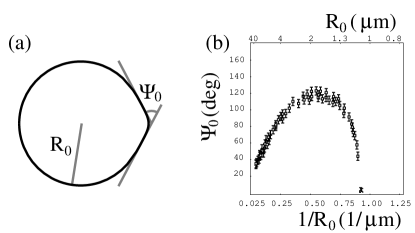
FIG. 8.: (a) The definition of the excluded angle $\Psi_{0}$. (b) Experimental measurements of the domain-size $R_{0}$ dependence of $\Psi_{0}$ observed in $L_{2}$ domains surrounded by LE phase taken from Ref. [9].

FIG. 9.: The shapes of domains of various sizes computed for $\sigma_{0}=4$, $a_{1}=1.6$ and $a_{2}=0.8$. (a)Smaller domains with $R_{0}=0.2$, $0.25$, $0.33$, $0.5$, $1$ which exhibit 2-fold symmetry. (b)Larger domains with $R_{0}=2$, $2.5$, $3.3$, $5$, $10$ which have a protrusion on one end of the boundary. Each of the sets of domains are plotted to scale.

To compare the theoretical results to the experimental data, a length scale is required. The length scale is set by the assignment $\kappa/a_{1}=4\mu m$ when the comparisons is made between the perturbative results and the experimental data [12]. Except for examining the results of more reliable computations, there is no attempt to fit the experimental data in this report for reasons to be discussed below. We first adopt the same set of parameters, with which the perturbative analysis fits the data in the large-$R_{0}$ regime, for the comparison. It is obvious from Fig. 10(b) that even at $\gamma=0.5$, the theoretical prediction for the maximum of $\Psi_{0}$ is much smaller than that observed experimentally. This superficial comparison between the maxima of $\Psi_{0}$ implies that $\gamma$ is very much larger in the system investigated. Detailed comparisons do show excellent agreement for domains larger than $10\mu m$. Experimentally observed domains with maximum $\Psi_{0}$ and small circular domains are not reproduced numerically. Attempts have been made to investigate the combined effect of elastic anisotropy $b$ and $\gamma$. However, for $\gamma$ of such a magnitude, contributions from the $b$ do not affect the qualitative behaviors discussed in this context. It is thus concluded that although the simple elastic modelis not capable of fully addressing the issue of the domain size dependence of the shapes, it has successfully produced the qualitative features in the $\Psi_{0}$ versus $R_{0}$ plot and many nontrivial domain shapes observed in various experiments[18].

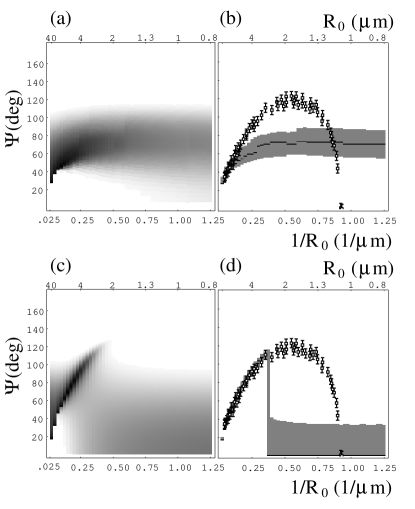
FIG. 10.: (a) Density plot of $I$ as a function of $\Psi$ and $R_{0}$ of the numerical results for the domains. (b) Plot of $I_{max}$ and the region in which $I>I_{max}/2$ as a function of $\Psi$ and $R_{0}$ of the numerical results for the domains. Superimposed are the experimental data shown in Fig. 8(b) with parameters $\kappa/a_{1}=4\mu m$, $\delta=0.4$ and $\gamma=0.5$. (c) and (d) are corresponding plots for the perturbative results.

In the large-$R_{0}$ regime ($R_{0}\gg 1$), the boundary corrections are confined in a small portion of the boundary and the domains become nearly circular. Because of the rapid texture variations in the immediate vicinity of the boundary, associated with the approach to the boundary of the virtual defect, we are unable to perform dependable numerical investigations of extremely large domains. This leaves open the question of the asymptotic behavior of $\Psi_{0}$ is the $R_{0}\rightarrow\infty$ limit.

With the numerical scheme for evaluating simultaneously ${\bf\Theta}$ and $\Gamma$. We are able to explore the simple model Eq. (1) in a much wider range of the parameter space with

confidence. Not only does the model account for the domains with various features observed in experiments, it also yields an appropriate domain size dependence of the boundary shapes. However, we are unable to perform reliable numerical investigations on extremely large domains. Despite the fact that there is an upper bound to the domain size that we are able to compute, we believe, on the basis of measurements of the defect positions [5] that the largest domains we are able to compute are not smaller than those that have been observed experimentally. The numerical algorithm appears to be capable of evaluating domain shapes for arbitrary anisotropic line-tension, with one caveat. A closer look at Eqs. (21) and (23) immediately indicates that this approach is not appropriate for situations in which $\sigma+\sigma^{\prime\prime}=0$ at some points on the boundary. An approach that is appropriate to this situation is the Wulff constructions [10].

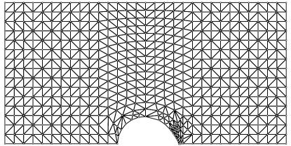
FIG. 11.: Mesh with additional external boundary used in the direct extension of the FEM algorithm for the bubbles.

IV bubbles

We now turn to the investigation of bubbles. The first task is to numerically evaluate the texture in a region, $\Omega$, that does not have an external boundary. It is possible to implement a straightforward extension of the problem of the domain by introducing an artificial external boundary far away from the inner bounding curve $\Gamma$. One must introduce a boundary condition on this added external boundary by hand. Figure  11 displays the triangulations associated with such implementation of the approach to the calculation of the property of a bubble. The method, though inefficient, produces results that are consistent with those obtained perturbatively [12].

The problem that involves an infinite $\Omega$ with internal boundary $\Gamma$ is referred to as the exterior problem. If one does not introduce an artificial external boundary, it is necessary to have at hand a complete set of exterior solutions to construct the boundary condition at $\Gamma$. For our particular case, this is possible when $b=0$, in which case the bulk extremum equation reduces to Laplace’s equation. The examination of the problem with nonzero $b$ is a major goal of this investigation, and we are not aware of the existence of an appropriate set of external solutions in this case. Noting that the order parameter tends to a fixed value ($\Theta=0$ for our case here) as $r\rightarrow\infty$, it is possible to approach the problem of the bubble using a different set of polar co-ordinates, i.e. $(r^{\prime},\varphi)\equiv(1/r,\varphi)$, that transform the bubble into a domain of area $\Omega^{\prime}$ and bounding curve $\Gamma^{\prime}$, shown in Fig. 12, with the following “elastic energy”,

$${\cal H}= \frac{\kappa}{2}\int_{\Omega^{\prime}}\left\{\Theta_{x}^{2}+\Theta_{y}^{2}+\beta\left[\left(-\Theta_{x}^{2}+\Theta_{y}^{2}\right)\cos 2(\Theta-2\varphi)\right.\right.$$ (25)

$$\left.\left.+2\Theta_{x}\Theta_{y}\sin 2(\Theta-2\varphi)\right]\right\}\,dA+\oint_{\Gamma^{\prime}}\frac{\sigma(\vartheta-\Theta)}{R^{-2}}\;ds$$

With the problem transformed, the meshing algorithm used for the domain can be applied immediately. We are then able to proceed with the investigation of the bubbles with the same efficiency and same accuracy as the studies of the domains.

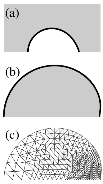
FIG. 12.: Solving the problem of the bubble by transforming it into an inverse domain problem. (a) shows the region $\Omega$ of ordered phase and the boundary $\Gamma$ for the bubble. (b) shows the transformed region $\Omega^{\prime}$ and boundary $\Gamma^{\prime}$. (c) shows the mesh that covers $\Omega^{\prime}$.

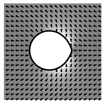
FIG. 13.: Boundaries and textures around the bubbles for $R_{0}=5$, $a_{1}=1$, $\kappa=1$ and $b=0$.

In the numerical studies that we have performed with the use of the transformation above, the results for the bubbles reported in the perturbative analysis [12, 7] that the boundaries are not circular even when $b=0$ and $a_{2}=0$, have been confirmed. Figure 13 shows the texture and the boundary of a typical bubble. In the background simulated BAM image, one notes the circular constant-intensity lines which identify the “inverse boojum”. The numerical algorithm further enables us to obtained equilibrium bubble boundaries and textures around them when elastic anisotropies are present. As can be seen in Fig. 14, the elastic anisotropy leaves the boundaries substantially unaffected while significantly changing the appearance of the textures around the bubbles. The BAM images are also shown in the same figures. In contrast to the case in which $b=0$, the constant-intensity lines become elongated perpendicular to the axis connecting the center of the bubble and the position of the virtual defect when $b<0$. These lines are elongated in the direction of the axis when $b>0$, as shown. This allows for the determination of the sign of $b$ in the Langmuir monolayer by examining the BAM images of the bubbles.

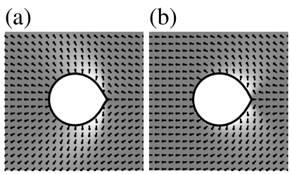
FIG. 14.: Boundaries and textures around the bubbles for $R_{0}=5$, $a_{1}=1$, $\kappa=1$, (a) with $b=-0.8$ and (b) $b=0.8$.

FIG. 15.: Boundaries of bubbles computed for $\kappa=0.16$, $\sigma_{0}=1$, $a_{1}=0.16$ and (a) $R_{0}=1$, $2$, $3$, $4$, $5$, $6$, and (b) $R_{0}=8$, $20$, $40$.

In Figs. 15, we display the size dependence of the bubble boundaries. Bubbles appear to be circular when they are small ($R_{0}<1$). For large enough bubbles ($R_{0}\geq 1$), an “excluded angle” $\Psi_{0}$ defined in Fig. 8(a) can be identified. An approach similar to the analysis of the size dependence of the boundary in the case of domains can be applied. Figures 16(a) and (c) compare the density plots of $I$ as a function of $\Psi$ versus $R_{0}$ for the numerical and the perturbative results. The two plots are in excellent agreement. When $\gamma=0$, the texture does not differ significantly from that of the inverse boojum even though the bubble is not exactly circular. This contrasts to what is seen in domains when $\gamma\neq 0$, in which case the textures can deviate significantly from the boojum texture. The $R_{0}$ dependence of $\Psi_{0}$ features that are qualitatively similar to those seen in the case of the domains, i.e. a maximum and an onset. These features have also been observed experimentally [7]. Experimental data is shown together with the numerical and perturbative results in Figs. 16(b) and (d), respectively, and all the results match reasonably well. The by-eye fit has been obtained in Ref. [7] and no further adjustment of the parameters is made in this investigation.

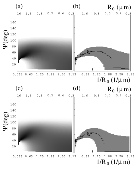
FIG. 16.: (a) Plot of $I$ as a function of $\Psi$ and $R_{0}$ of the numerical results for the bubbles. (b) Plot of $I_{max}$ and the region in which $I>I_{max}/2$ as a function of $\Psi$ and $R_{0}$ of the numerical results for the bubbles. Superimposed are the experimental observations of gaseous bubbles in $L_{2}$ phase. The experimental data have appeared in Ref. [9]. The parameters for the by-eye fit are $\kappa/a_{1}=0.4\mu m$ and $\delta=0.16$. (c) and (d) are the corresponding plots for the perturbative results.

We have thus devised a numerical method to approach the problem of the bubble that can be implemented with the same efficiency as in the problem of the domain. There is good agreement between perturbative and numerical results. We are able to investigate the effect of the elastic anisotropy, and our results point to a possible means for the determination of the relative strength of $K_{s}$ and $K_{b}$.

V conclusions

We have discussed in this report the implementation of a numerical method that leads us to the solution of simultaneous equilibrium conditions for the textures and the bounding curve of the domains. Using this numerical algorithm, we have investigated the influences on the textures and the domain shapes of the line-tension and elastic anisotropies. Our analysis of this simple model reveals that elastic anisotropy does, indeed, result in interesting domain boundaries with protrusions and indentations. The domains with indentations resemble those observed experimentally. However, the domains that we generate with protrusions are very different from those in observed in BAM images[18]. Hence, elastic anisotropy cannot qualitatively account for all experimental observations. Furthermore, our numerical results are in contrast to the claims in Ref. [11]. Dents in boundaries are due to a bend modulus that exceeds the splay modulus, i.e. $b\equiv(K_{s}-K_{b})/(K_{s}+K_{b})<0$, while protrusions are present when $b>0$. On the other hand, the second harmonic contribution to the line-tension, parameterized by $\gamma\equiv a_{2}/a_{1}$ is capable of producing nontrivial domain shapes that resemble the shapes observed experimentally. For the influence of $\gamma$ on the boundary, our results are in qualitative agreement with those presented in Ref. [11]. Comparison has also been made between perturbative results [12], the numerical computations described here and the experimental data[7]. The magnitude of $\gamma$ used in the perturbative analysis is the prime factor causing the mismatch between the perturbative and the numerical results. When $\gamma$ is large (=0.5 for our case), the first order perturbative approach is not expected to be accurate.

While the results of the perturbative analysis and the numerical study are different quantitatively, they possess similar qualitative features, namely the onset of the excluded angle $\Psi_{0}$ as the domain size $R_{0}$ increases, and then $\Psi_{0}$ reaches a maximum of and then decrease as $R_{0}$ continues to increase. These match the qualitative features that are present the experimental data [7] shown in Fig. 8(b). Experimental results is not reproduced in the numerical calculations when $R_{0}$ is small. The discrepancies between the experimental data and the numerical result imply that other interactions, neglected in the model, may be significant.

We have also extended the numerical algorithm to the problem of bubbles. It is found that the transformation $r\rightarrow r^{\prime}\equiv 1/r$ results in a new domain problem which allows us to solve the equilibrium conditions for the bubbles at the same level of efficiency and accuracy as those for the domains. Not only have we obtained results that are consistent with those in the perturbative analysis  [7, 12], we have also analyzed the effect of elastic anisotropy on the textures and the boundary of the bubbles, a task that is algebraically formidable in the perturbative analysis. The influence of elastic anisotropy on the boundary is small while it significantly modifies the textures. This provides a means for the qualitative determination of the elastic anisotropy by observing the texture around the bubbles. The agreement between the perturbative results and the numerical computation is excellent. This is not surprising as $a_{2}$ is not involved. The $R_{0}$ dependence of $\Psi_{0}$ is similar to the case of the domain, except that the maximum of $\Psi_{0}$ is much smaller. The perturbative result agrees reasonably with the experimental data as reported in Ref. [7]. The numerical results match as well.

In conclusion, we have successfully implemented a numerical algorithm that enable us to analyze unambiguously a simple model, Eq.(1), of tilted ordered media in a non-trivial geometry imposed by experimental observations. Using this numerical algorithm and its extensions, we are able to address the long-standing debate with regard to the origin on the cusp-like features observed in domains of Langmuir monolayers using an elastic model. Within the context of this simple model which addresses only the competition between the bulk elastic energy and the boundary energy, many qualitative features of the experimental observation have been captured. Discrepancies cannot be avoided, as the real system is much more complex. The model we adopted has neglected other effects and interactions that are present in real system, such as dipolar interactions and adjustments in the tilt degree of freedom. A combination of these effects may account for the discrepancies between the experimental data and the theoretical results. The apparently general numerical algorithm is, however, not capable of handling situation in which $\sigma+\sigma^{\prime\prime}=0$ at some points on the boundary. A different approach, such as the Wulff construction[10], is required. Nevertheless, our numerical algorithm is versatile and can be extended to systems containing topological defects, or with the ordered phase filled in a nonsimply connected space.

A Variational formulation of the FEM

In finite element analysis, we approximate $\Theta(x,y)$ by Eq. (10). The energy functional $H[\Theta]$ given in Eq. (1) now becomes

$$H({\bf\Theta}) = \frac{\kappa}{2}\int_{\Omega}\left\{|\nabla\Theta|^{2}+b\left[\left(-\Theta_{x}^{2}+\Theta_{y}^{2}\right)\cos 2\Theta-\right.\right.$$ (A2)

$$\left.\left.2\Theta_{x}\Theta_{y}\sin 2\Theta\right]\right\}\;dA\oint_{\Gamma}\sigma(\vartheta-\Theta)\;ds$$

where we denote ${\bf\Theta}\equiv(\Theta_{1},\Theta_{2},\cdots,\Theta_{N})^{T}$, and $\Theta=\sum\varphi_{i}\Theta_{i}$. We differentiate Eq. (A2) with respect to a $\Theta_{i}$ yields

$$\frac{\partial H({\bf\Theta})}{\partial\Theta_{i}} = \kappa\int_{\Omega}[\varphi_{ix}\varphi_{jx}(1-b\cos 2\Theta)+$$ (A7)

$$\varphi_{iy}\varphi_{jy}(1+b\cos 2\Theta)+$$

$$b(\varphi_{ix}\varphi_{jy}+\varphi_{iy}\varphi_{jx})\sin 2\Theta]dA\Theta_{j}$$

$$-\kappa b\int_{\Omega}[(-\Theta_{x}^{2}+\Theta_{y}^{2})\sin 2\Theta+$$

$$2\Theta_{x}\Theta_{y}\cos 2\Theta]\varphi_{i}dA-\oint_{\Gamma}\sigma^{\prime}(\vartheta-\Theta)\varphi_{i}ds$$

The equilibrium condition gives ${\bf A}{\bf\Theta}={\bf b}$ with ${\bf A}$ and ${\bf b}$ provided in Eqs. (16) and (19).

B Integration over a triangulation

The integrals in Eqs. (16) and (19) over $\Omega$ are broken up into sums of integration over the triangles in the triangulation of $\Omega$. Integration over the interior individual triangle can usually be carried out analytically depending on the specific forms of the basis functions $\varphi_{i}(x,y)$ and the matrix elements $A_{ij}$ and $b_{i}$. We have chosen $\varphi_{i}(x,y)$ to be a continuous, piecewise linear function in $x$ and $y$ within a triangle. The line integral $\oint_{\Gamma}ds$ in $b_{i}$ will must be evaluated numerically, because integrand depends on the polar angle $\varphi$, which is not linear in $x$ or $y$. This does not degrade the efficiency of the computation because first of all, only triangles whose perimeters coincide with $\Gamma$ contribute to the line integral and secondly it is a line integral over a short distance.

In Eq. (10), we express a function $f(x,y)$ for $(x,y)\in\Omega$ in terms of its values at the nodes of the triangulation and the corresponding basis functions $\varphi_{i}(x,y)$. Within an individual triangle $K$, we can write

$$f(x,y)=\sum_{i=1}^{3}f_{K_{i}}\varphi^{(K)}_{K_{i}}(x,y)$$ (B1)

where $K_{i}$ is the index of the $i$th vertex of the triangle $K$, $f_{K_{i}}=f(x_{K_{i}},y_{K_{i}})$, $(x_{K_{i}},y_{K_{i}})$ are respectively the functional value of $f(x,y)$ and the coordinates of the $i$th vertex. $\varphi^{(K)}_{K_{i}}(x,y)$ is the restriction of $\varphi_{K_{i}}(x,y)$ in $K$. The actual index of the $i$th vertex is $K_{i}$. It is, however, awkward to carry the $K$ in the symbol $K_{i}$ throughout the discussion. We will use $i$ to identity the vertex for simplicity from now on, i.e. $f_{K_{i}}$ is simplified as $f_{i}$. We introduce a set of natural coordinates $u$ and $v$ such that

$$f(u,v)=f_{1}+(f_{2}-f_{1})u+(f_{3}-f_{1})v,$$ (B2)

where $u\in[0,1]$, $v\in[0,1]$ and $u+v\leq 1$. Transformation between variable sets $x-y$ and $u-v$ can be obtained from Eq. (B2) by substituting $f$ with $x$ and $y$. We then have the followings relations

$$u= \frac{1}{\Delta}\left[\left(y_{3}-y_{1}\right)x-\left(x_{3}-x_{1}\right)y+x_{3}y_{1}-x_{1}y_{3}\right],$$ (B3)

$$v= \frac{1}{\Delta}\left[\left(y_{1}-y_{2}\right)x-\left(x_{1}-x_{2}\right)y+x_{1}y_{2}-x_{2}y_{1}\right],$$ (B4)

where $\Delta$ is the Jacobian determinant given by

$$\Delta=\frac{\partial(x,y)}{\partial(u,v)}=x_{1}y_{2}-y_{1}x_{2}+x_{2}y_{3}-x_{3}y_{2}+x_{3}y_{1}-x_{1}y_{3}.$$ (B.5)

Identifying Eqs. (B1) and (B2), we find $\varphi_{1}(u,v)=1-u-v$, $\varphi_{2}(u,v)=u$ and $\varphi_{3}(u,v)=v$. In terms of $x-y$, we have

$$\varphi_{1}(x,y)= \frac{1}{\Delta}\left[\left(y_{2}-y_{3}\right)x-\left(x_{2}-x_{3}\right)y+x_{2}y_{3}-x_{3}y_{2}\right],$$ (B.6)

$$\varphi_{2}(x,y)= \frac{1}{\Delta}\left[\left(y_{3}-y_{1}\right)x-\left(x_{3}-x_{1}\right)y+x_{3}y_{1}-x_{1}y_{3}\right],$$ (B.7)

$$\varphi_{3}(x,y)= \frac{1}{\Delta}\left[\left(y_{1}-y_{2}\right)x-\left(x_{1}-x_{2}\right)y+x_{1}y_{2}-x_{2}y_{1}\right].$$ (B.8)

Evaluation of the matrix element $A_{ij}$ involves of the following area integrals which can be computed analytically. The trivial one is the area of $K$, which is $\int_{K}\;dA=|\Delta|/2$ and

$$\int_{K}\cos 2\Theta\;dA= \frac{|\Delta|}{4}\left[\frac{\cos 2\Theta_{1}}{(\Theta_{1}-\Theta_{2})(\Theta_{2}-\Theta_{3})}+\frac{\cos 2\Theta_{2}}{(\Theta_{2}-\Theta_{3})(\Theta_{3}-\Theta_{1})}+\frac{\cos 2\Theta_{3}}{(\Theta_{3}-\Theta_{1})(\Theta_{1}-\Theta_{2})}\right],$$ (B.9)

$$\int_{K}\sin 2\Theta\;dA= \frac{|\Delta|}{4}\left[\frac{\sin 2\Theta_{1}}{(\Theta_{1}-\Theta_{2})(\Theta_{2}-\Theta_{3})}+\frac{\sin 2\Theta_{2}}{(\Theta_{2}-\Theta_{3})(\Theta_{3}-\Theta_{1})}+\frac{\sin 2\Theta_{3}}{(\Theta_{3}-\Theta_{1})(\Theta_{1}-\Theta_{2})}\right],$$ (B.10)

as $\varphi_{ix}$ and $\varphi_{iy}$ are constants. Evaluation of $b_{i}$ involves

$$\int_{K}\varphi_{1}\cos 2\Theta\;dA= \frac{|\Delta|}{4}\left[\frac{\cos 2\Theta_{1}}{(\Theta_{3}-\Theta_{1})(\Theta_{1}-\Theta_{2})}+\frac{\sin 2\Theta_{1}-\sin 2\Theta_{3}}{2(\Theta_{1}-\Theta_{3})^{2}(\Theta_{3}-\Theta_{2})}-\frac{\sin 2\Theta_{1}-\sin 2\Theta_{2}}{2(\Theta_{1}-\Theta_{2})^{2}(\Theta_{3}-\Theta_{2})}\right],$$ (B.11)

$$\int_{K}\varphi_{2}\cos 2\Theta\;dA= \frac{|\Delta|}{4}\left[\frac{\cos 2\Theta_{2}}{(\Theta_{1}-\Theta_{2})(\Theta_{2}-\Theta_{3})}+\frac{\sin 2\Theta_{2}-\sin 2\Theta_{3}}{2(\Theta_{2}-\Theta_{3})^{2}(\Theta_{3}-\Theta_{1})}-\frac{\sin 2\Theta_{2}-\sin 2\Theta_{1}}{2(\Theta_{1}-\Theta_{2})^{2}(\Theta_{3}-\Theta_{1})}\right],$$ (B.12)

$$\int_{K}\varphi_{3}\cos 2\Theta\;dA= \frac{|\Delta|}{4}\left[\frac{\cos 2\Theta_{3}}{(\Theta_{2}-\Theta_{3})(\Theta_{3}-\Theta_{1})}+\frac{\sin 2\Theta_{3}-\sin 2\Theta_{2}}{2(\Theta_{2}-\Theta_{3})^{2}(\Theta_{2}-\Theta_{1})}-\frac{\sin 2\Theta_{3}-\sin 2\Theta_{1}}{2(\Theta_{1}-\Theta_{3})^{2}(\Theta_{3}-\Theta_{1})}\right],$$ (B.13)

$$\int_{K}\varphi_{1}\sin 2\Theta\;dA= \frac{|\Delta|}{4}\left[\frac{\sin 2\Theta_{1}}{(\Theta_{3}-\Theta_{1})(\Theta_{1}-\Theta_{2})}-\frac{\cos 2\Theta_{1}-\cos 2\Theta_{3}}{2(\Theta_{1}-\Theta_{3})^{2}(\Theta_{3}-\Theta_{2})}+\frac{\cos 2\Theta_{1}-\cos 2\Theta_{2}}{2(\Theta_{1}-\Theta_{2})^{2}(\Theta_{3}-\Theta_{2})}\right],$$ (B.14)

$$\int_{K}\varphi_{2}\sin 2\Theta\;dA= \frac{|\Delta|}{4}\left[\frac{\sin 2\Theta_{2}}{(\Theta_{1}-\Theta_{2})(\Theta_{2}-\Theta_{3})}-\frac{\cos 2\Theta_{2}-\cos 2\Theta_{3}}{2(\Theta_{2}-\Theta_{3})^{2}(\Theta_{3}-\Theta_{1})}+\frac{\cos 2\Theta_{2}-\cos 2\Theta_{1}}{2(\Theta_{1}-\Theta_{2})^{2}(\Theta_{3}-\Theta_{1})}\right],$$ (B.15)

$$\int_{K}\varphi_{3}\sin 2\Theta\;dA= \frac{|\Delta|}{4}\left[\frac{\sin 2\Theta_{3}}{(\Theta_{2}-\Theta_{3})(\Theta_{3}-\Theta_{1})}-\frac{\cos 2\Theta_{3}-\cos 2\Theta_{2}}{2(\Theta_{2}-\Theta_{3})^{2}(\Theta_{2}-\Theta_{1})}+\frac{\cos 2\Theta_{3}-\cos 2\Theta_{1}}{2(\Theta_{1}-\Theta_{3})^{2}(\Theta_{3}-\Theta_{1})}\right].$$ (B.16)

The above formulae will work only if $\Theta_{1}\neq\Theta_{2}\neq\Theta_{3}$. Let us consider cases where the values of $\Theta=\Theta_{E}$ at 2 vertices of triangle $K$ and $\Theta=\Theta_{O}$ at the other vertex. We obtain the following for the integrals in $A_{ij}$

$$\int_{K}\cos 2\Theta\;dA = \frac{|\Delta|}{4}\left[\frac{\cos 2\Theta_{E}-\cos 2\Theta_{O}}{(\Theta_{E}-\Theta_{O})^{2}}+\frac{2\sin 2\Theta_{E}}{\Theta_{E}-\Theta_{O}}\right]$$ (B.17)

$$\int_{K}\sin 2\Theta\;dA = \frac{|\Delta|}{4}\left[\frac{\sin 2\Theta_{E}-\sin 2\Theta_{O}}{(\Theta_{E}-\Theta_{O})^{2}}-\frac{2\cos 2\Theta_{E}}{\Theta_{E}-\Theta_{O}}\right]$$ (B.18)

We denote $\varphi_{E}$ the restrictions of the basis functions at the nodes that have $\Theta=\Theta_{E}$, and $\varphi_{O}$ the restriction of the basis function at the node that has $\Theta=\Theta_{O}$. We arrive at

$$\int_{K}\varphi_{E}\cos 2\Theta\;dA = \frac{|\Delta|}{4}\left[\frac{\sin 2\Theta_{E}}{\Theta_{E}-\Theta_{O}}+\frac{\cos 2\Theta_{E}}{(\Theta_{E}-\Theta_{O})^{2}}-\frac{\sin 2\Theta_{E}-\sin 2\Theta_{O}}{2(\Theta_{E}-\Theta_{O})^{3}}\right]$$ (B.19)

$$\int_{K}\varphi_{O}\cos 2\Theta\;dA = \frac{|\Delta|}{4}\left[-\frac{\cos 2\Theta_{E}+\cos 2\Theta_{O}}{(\Theta_{E}-\Theta_{O})^{2}}+\frac{\sin 2\Theta_{E}-\sin 2\Theta_{O}}{(\Theta_{E}-\Theta_{O})^{3}}\right]$$ (B.20)

$$\int_{K}\varphi_{E}\sin 2\Theta\;dA = \frac{|\Delta|}{4}\left[-\frac{\cos 2\Theta_{E}}{\Theta_{E}-\Theta_{O}}+\frac{\sin 2\Theta_{E}}{(\Theta_{E}-\Theta_{O})^{2}}+\frac{\cos 2\Theta_{E}-\cos 2\Theta_{O}}{2(\Theta_{E}-\Theta_{O})^{3}}\right]$$ (B.21)

$$\int_{K}\varphi_{O}\sin 2\Theta\;dA = \frac{|\Delta|}{4}\left[-\frac{\sin 2\Theta_{E}+\sin 2\Theta_{O}}{(\Theta_{E}-\Theta_{O})^{2}}-\frac{\cos 2\Theta_{E}-\cos 2\Theta_{O}}{(\Theta_{E}-\Theta_{O})^{3}}\right]$$ (B.22)

for the integrals required to evaluate $b_{i}$. Finally, when $\Theta_{i}=\Theta_{E}$ for all $i$’s, one will need $\int_{K}\varphi_{E}\;dA=|\Delta|/6$.

C Derivatives on the boundary

One of the biggest benefits of the FEM is that it enables straightforward determination of the derivatives of $\Theta$ on the boundary. The tangential derivative at node $i$ as

$$\left.\frac{\partial\Theta}{\partial t}\right|_{i}=\frac{1}{2e^{k}\sqrt{1+k^{\prime 2}}}\left[\frac{\Theta_{i+1}-\Theta_{i}}{\varphi_{i+1}-\varphi_{i}}+\frac{\Theta_{i}-\Theta_{i-1}}{\varphi_{i}-\varphi_{i-1}}\right]$$ (C.1)

The normal derivative of $\Theta$ is given by Eq. (7) which reads

$$\frac{\partial\Theta}{\partial n}=\frac{e^{k}\sigma^{\prime}(\vartheta-\Theta)+\kappa b\Theta_{t}\sin 2(\Theta-\vartheta)}{\kappa[1-b\cos 2(\Theta-\vartheta)]}.$$ (C.2)

REFERENCES

- [1] C.M. Knobler and R.C. Desai, Annu. Rev. Phys. Chem. 43, 207 (1992).
- [2] J. Ruiz-Garcia, X. Qiu, M.-W. Tsao, G. Marshall, C.M. Knobler, G. A. Overbeck and D. Möbius, J. Phys. Chem 97, 6955 (1993); D.K. Schwartz, J.Ruiz-Garcia, X. Qiu, J.V. Seligner and C.M. Knobler, Physica A 204, 606 (1994);J.V. Selinger, Z.-G. Wang, R.F. Bruinsma and C.M. Knobler, Phys. Rev. Lett. 70, 1139 (1993).
- [3] X. Qiu, J. Ruiz-Garcia, K. J. Stine, C.M. Knobler, J.V. Selinger, Phys. Rev. Lett. 67 703 (1991).
- [4] T.M. Fischer, R.F. Bruinsma and C.M. Knobler, Phys. Rev. E 50, 413 (1994).
- [5] S. Rivière and J. Meunier, Phys. Rev. Lett. 74, 2495 (1995).
- [6] N.D. Mermin, in Quantum Fluids and Solids, edited by S.B. Trickey, E. Adams and J. Duffy (Plenum, New York, 1977).
- [7] J. Fang, E. Teer, C.M. Knobler, K.-K. Loh and J. Rudnick, Phys. Rev. E 56, 1859 (1997).
- [8] S.A. Langer and J.P. Sethna, Phys. Rev. A 34, 5035 (1986).
- [9] I. Kraus and R.B. Meyer, Phys. Rev. Letts 81, 3815 (1999).
- [10] J. Rudnick and R. Bruinsma, Phys. Rev. Lett. 74, 2491 (1995).
- [11] P. Galatola and J.B. Fournier, Phys. Rev. Lett. 75, 3297 (1995).
- [12] J. Rudnick and K.-K. Loh, Phys. Rev. E 60, 3045 (1999).
- [13] C. Johnson, Numerical solution of partial differential equations by the finite element method (Cambridge University Press, Cambridge, 1987).
- [14] W.H. Press, B.P. Flannery, S.A. Tuekolsky and W.T. Vetterling, Numerical Recipes in C, The Art of Scientific Computing (Cambridge University Press, Cambridge, 1991).
- [15] K.-K. Loh and J. Rudnick, Phys. Rev. Lett. 81, 4935 (1998).
- [16] D. Pettey and T.C. Lubensky, Phys. Rev. E 59, 1834 (1999).
- [17] E. Teer and C.M. Knobler, private communications; C. Lautz, T.M. Fischer, M. Weygand, M. Lösche, P.B. Howes and K. Kjaer, J. Chem. Phys. 108, 4640 (1998).
- [18] J. Fang and C.M. Knobler, unpublished.