Multiple-scattering effects on smooth neutron spectra

Abstract

Elastic and inelastic incoherent neutron scattering experiments are simulated for simple models: a rigid solid (as used for normalisation), a glass (with a smooth distribution of harmonic vibrations), and a viscous liquid (described by schematic mode-coupling equations). As long as the spectral distribution of the input scattering law does not vary with wavenumber, it is only weakly distorted by multiple scattering. The wavenumber dependence of the scattering intensity suffers much more.

I Introduction

Any neutron scattering measurement is unavoidably contaminated by multiple scattering. For intensity reasons, samples must be chosen so thick that a significant fraction of the incident neutrons is scattered. As an inevitable consequence, a significant fraction of the scattered neutrons is scattered more than once.

In crystals, single scattering gives rise to discrete peaks that can be distinguished fairly well from a smooth background caused by multiple scattering. In amorphous solids and liquids, on the other hand, the dynamic structure factor $S(q,\nu)$ itself is a smooth function of wavenumber $q$ and frequency $\nu$. In this case, the multiple-scattering background cannot be removed by routine operations, and often it presents the limiting uncertainty in the data analysis.

Multiple scattering is basically a convolution of $S(q,\nu)$ with itself, and therefore it is nonlinear in $S$, and worse: it is nonlocal in $q$ and $\nu$. For this reason, multiple-scattering corrections are much more difficult than all the other manipulations that are necessary for deriving $S(q,\nu)$ from the counts $N(2\theta,\nu)$ measured at given detector angles $2\theta$: normalisation to the incident flux, subtraction of container scattering, correction for self-absorption, calibration to an incoherent standard scatterer, correction for the energy-dependent detector efficiency, and interpolation from constant-$2\theta$ to constant-$q$ cuts.

The nonlinearity of multiple scattering means that any correction requires $S(q,\nu)$ to be known in absolute units. The nonlocality means that a multiple-scattering event registered in a channel $2\theta,\nu$ results from a succession of scattering events at other angles and frequencies $2\theta_{i},\nu_{i}$ ($i=1,2,\ldots$). Corrections are only possible if $S(q,\nu)$ is known over a wide range in $q$ and $\nu$. Some of the multiple-scattering sequences that contribute to $N(2\theta,\nu)$ involve even angles or frequencies that are not covered directly in the given experiment. Therefore, it is impossible to infer the distribution of multiple-scattering from the measured $N(2\theta,\nu)$ alone. A full treatment of multiple scattering requires an extension of the measured scattering law into a wider $q,\nu$ domain.

In a pragmatic approach, this extension is provided either by somehow extrapolating the measured data or by fitting a more or less physical model to them. Feeding the extended scattering law into a simulation one can estimate the multiple-scattering contribution, and subtract it from the measured data. After a few iterations one expects to obtain a reasonably corrected scattering law. Though such a procedure is regularly employed by a number of researchers, it never became part of the standard raw data treatment. The technical intricacies and inherent uncertainties of multiple-scattering corrections are rarely discussed in detail, and for the uninitiated it is almost impossible to assess their reliability.

The present work follows an alternative route: by performing extensive simulations on very simple model systems we shall try to identify some generic trends of multiple scattering. Ideally our results will help to assess past experiments and to plan future ones. Since we do not intend to correct data from a specific measurements, we choose the simplest sample geometry, and we do not consider scattering from the container.

We expect multiple scattering to be particularly harmful when the scattering law varies only weakly with $q$ and $\nu$, because small distortions of $S(q,\nu)$ suffice to destroy much of the information we are interested in. To investigate such situations, we consider incoherent scattering from a number of dynamic models. The scattering laws will be defined by closed mathematical expressions that cover the full $q,\nu$ plane, thereby guaranteeing correct normalisation. To keep the models in touch with reality, the choice of parameters will be inspired by actual experiments on organic glasses and liquids.

We start with simulating the vanadium or low-temperature scans needed for normalisation of the elastic scattering intensity. We then proceed with elastic and inelastic scattering from a simple harmonic system. This case has already been discussed more or less explicitely in experimental studies of amorphous solids [1, 2, 3, 4, 5].

In liquids, diffusion or slow relaxation cause the elastic part of the scattering law to broaden into a quasielastic $\alpha$ peak. Multiple-scattering effects in this regime have been studied occasionally [6, 7, 8]. More recently, interest has grown in the moderately viscous state above the cross-over temperature $T_{\rm c}$ of mode-coupling theory [9, 10] where a relatively narrow $\alpha$ peak is separated from the vibrational and relaxational high-frequency spectra by the intermediate regime of fast $\beta$ relaxation. By explicit integration of a schematic mode-coupling model we construct an $S(q,\nu)$ which can be used as input to the multiple-scattering simulation.

II Modelling $S(q,\nu)$

A Rigid model

The rigid model represents a completely frozen, perfectly incoherent scatterer

$$S(q,\nu)=\delta(\nu)\,.$$ (1)

Quantum-mechanical ground-state oscillations will be neglected. This model serves to simulate normalisation scans. The need for such simulations will become apparent in section IV A.

B Glass model

The glass model describes an isotropic assembly of harmonic oscillators. The ideal scattering law $S(q,\nu)$ is calculated by explicit Fourier transform of

$$S(q,t)={\rm e}^{-2W(q,0)}{\rm e}^{2W(q,t)}\,.$$ (2)

In the high-temperature limit the exponents are given by

$$2W(q,t)={\hbar^{2}q^{2}\over 6Mk_{\rm B}T}\int\!{\rm d}\nu\,{\rm e}^{-i2\pi\nu t}{\left({k_{\rm B}T\over h\nu}\right)}^{2}g(|\nu|)\,.$$ (3)

where $T$ is the temperature of the sample and $M$ the average mass of the atoms. Since the sharp cut-off of the Debye-model leads to overshots in the Fourier transform, it is preferable to assume a smooth density of states,

$$g(\nu)={9\nu^{2}\over{\nu_{\rm D}}^{3}}\,\exp\left({-\left({9\pi\over 16}\right)^{1/3}\left({\nu\over{\nu_{\rm D}}}\right)^{2}}\right)\,.$$ (4)

The Debye frequency $\nu_{\rm D}={\left({3n/4\pi}\right)}^{1/3}c$ depends on the atomic density $n$ and the sound velocity $c$ which has to be calculated as an average $\langle c^{-3}\rangle^{-1/3}$ over the longitudinal and transverse modes. For this model, the mean-square displacement can be calculated:

$${r_{0}}^{2}=2W(q,0)/q^{2}={\left({9\pi\over 2}\right)}^{1/3}{k_{\rm B}T\over M{(2\pi\nu_{\rm D})}^{2}}\,.$$ (5)

The parameter set

$$\begin{array}[]{@{}lcl}n&=&10^{23}\mbox{ cm}^{-3}\,,\\[6.45831pt] c&=&1.2\mbox{ km/s}\,,\\[6.45831pt] M&=&7.1\mbox{ a.m.u., and}\\[6.45831pt] T&=&150\mbox{ K}\end{array}$$ (6)

models reasonably well an organic molecular or polymeric glass; it leads to a displacement $r_{0}=0.3$ Å and to a Debye frequency $\nu_{\rm D}=3.46$ THz.

C Liquid model

The liquid model is defined by a simple mode-coupling model

$$\begin{array}[]{@{}lcl}0&=&\ddot{\phi}_{x}(t)+\eta_{x}\dot{\phi}_{x}(t)+{\Omega_{x}}^{2}\phi_{x}(t)\\[9.47217pt] &&\displaystyle+{\Omega_{x}}^{2}\int_{0}^{t}\!{\rm d}t^{\prime}\,m_{x}(\{\phi\},t-t^{\prime})\dot{\phi}_{x}(t^{\prime})\end{array}$$ (7)

where the subscript $x$ denotes either density correlations around the structure factor maximum ($x=0$), or tagged-particle correlations at different wavenumbers ($x=q$). The characteristic frequencies $\Omega_{x}$ set the time scale; the friction term $\eta_{x}\dot{\phi}_{x}$ stands for fast force fluctuations that have no influence on the long-time dynamics.

With the initial conditions

$$\phi_{x}(0)=1\,,\quad\dot{\phi}_{x}(0)=0$$ (8)

and the memory kernel of the $F_{12}$ model [9, 11],

$$m_{0}(\{\phi\},t)=v_{1}\phi_{0}(t)+v_{2}{\phi_{0}(t)}^{2}\,,$$ (9)

the collective dynamics $\phi_{0}(t)$ is fully determined by the coupling coefficients $v_{1}(T)$, $v_{2}(T)$. The tagged-particle correlators $\phi_{q}$, on the other hand, are driven by $\phi_{0}$. The simplest, bilinear coupling

$$m_{q}(\{\phi\},t)=v_{q}\phi_{0}(t)\phi_{q}(t)$$ (10)

is designated as Sjögren model [12]. The incoherent scattering law $S(q,\nu)$ is obtained by Fourier transform of $\phi_{q}(t)$.

The most striking prediction of mode-coupling theory is probably the existence of an intermediate scaling regime between $\alpha$ relaxation and microscopic vibrations, where all time correlation functions $\phi_{x}$ slow down towards a plateau $f_{x}$ [13]. Around this plateau, they factorize as

$$\phi_{x}(t)-f_{x}=h_{x}g_{\lambda}(t/t_{\sigma})\,.$$ (11)

The shape of the universal scaling function $g_{\lambda}$ depends on just one global parameter $\lambda$. Further predictions are made for the critical temperature dependence of $h_{x}$ and $t_{\sigma}$. Many neutron scattering experiments [3, 14, 15, 16, 17, 18, 19, 20, 21, 22] have been undertaken to test these predictions. However, the asymptotic law (11) holds only in a restricted frequency range, and therefore it cannot be used as input to a multiple-scattering calculation.

In the last couple of years it became possible to calculate the full evolution of $\phi_{x}(t)$ very efficiently and to arbitrarily long times by explicit integration in the time domain [23, 24]. In cases where the asymptotic regime is not reached numeric solutions of schematic mode-coupling models have been used to fit experimental data [25, 26, 27, 28]. In a most recent example data from incoherent neutron scattering [22], depolarized light scattering [22, 29] and dielectric spectroscopy [30] on glass-forming propylene carbonate have been analysed first in terms of scaling [22] and then by integration of the $F_{12}$–Sjögren model, where the different observables were all governed by one and the same density correlator $\phi_{0}(t)$ [31]. Results from these fits will now be used to construct a realistic $S(q,\nu)$ as input to a multiple-scattering simulation.

We arbitrarily select the 220 K data which could be fitted with the following set of parameters [31, 32, 33]:

$$\begin{array}[]{@{}lcl}\Omega_{0}&=&1000\mbox{ GHz}\,,\\[1.29167pt] \Omega_{q}&=&q\cdot 224\mbox{ GHz / \AA}^{-1}\,,\\[1.29167pt] \eta_{0}&=&0\,,\\[1.29167pt] \eta_{q}&=&350\mbox{ GHz}\,,\\[1.29167pt] v_{1}&=&0.83\,,\\[1.29167pt] v_{2}&=&1.66\,.\end{array}$$ (12)

Deviating from Ref. [31], the $q$-dependent vertices in the Sjögren coupling (10) are determined from

$$1/(v_{q}f_{0})=1-\exp(-{r_{0}}^{2}q^{2})$$ (13)

with $r_{0}=0.546$ Å, which satisfies the physical requirements $1\!-\!f_{q}\sim q^{2}$ and $h_{q}\sim q^{2}$ for $q\to 0$ as well as $f_{q}\to 0$ for $q\to\infty$ [34].

III Monte-Carlo simulation

A Algorithm

The multiple-scattering simulation consists essentially of a Monte-Carlo integration over many neutron trajectories. The program basically follows the well documented Mscat algorithm [35, 36, 37]. All restrictions on storage size could be lifted; the quasielastic scattering law was stored on logarithmic $q$ and $\nu$ grids with about $40\times 240$ entries. Runs with $10^{4}$ to $10^{6}$ neutrons on a medium-size workstation took between less than a minute and several hours.

Each neutron is initialized with an energy $E_{0}$ and a direction ${\bf\hat{k}}_{0}$ along the incident beam. Since we are not interested in instrumental resolution effects, the option of choosing $E_{0}$ and ${\bf\hat{k}}_{0}$ from finite distributions is not used. Next, the impact point ${\bf r}_{0}$ on the sample surface is chosen at random, and the length $l({\bf r}_{0},{\bf\hat{k}}_{0})$ of a trajectory straight across the sample is calculated. Given the total scattering cross section density $\Sigma(E_{0})$, the neutron will be scattered somewhere within the sample with a probability $p_{0}=\exp(-\Sigma(E_{0})l({\bf r}_{0},{\bf\hat{k}}_{0}))$. With a probability $1-p_{0}$, the neutron will traverse the sample without interaction; absorption shall not be considered. At this point, the algorithm forces all neutrons to be scattered within the sample, assigning them as a weight $w_{0}$ the survival probability $p_{0}$. A collision point ${\bf r}_{1}$ is chosen at a distance $l$ from ${\bf r}_{0}$ with a probability proportional to ${\rm d}\exp(-\Sigma(E_{0})l)/{\rm d}l$, and a new energy $E_{1}$ and direction ${\bf\hat{k}}_{1}$ are selected according to the ideal scattering law $S(q,\nu)$. Then, the distance $l({\bf r}_{1},{\bf\hat{k}}_{1})$ to be travelled upon leaving the sample is calculated, the neutron is assigned a new weight $w_{1}=w_{0}p_{1}$, and the whole procedure is iterated.

For each collision $i=1,2,\ldots$, the contribution of the neutron to the scattering score $S_{(i)}(2\theta,\nu)$ is evaluated for all detector angles and for all energy channels. The weight of each contribution is a product of (i) the weight $w_{i-1}$, (ii) the scattering law that brings the neutron from its previous state into the segment $q,\nu$, and (iii) the probability of reaching the detector without further collsions.

With each collision the neutron looses weight. Following its trajectory too far would make the simulation inefficient. Therefore, when the weight $w_{i}$ falls below a predefined threshold $w_{\rm c}$, the neutron’s fate is determined by a Russian roulette: with a probability $1/2$ its weight is doubled, otherwise the trajectory has come to an end.

B Setup

Samples have most often the form of a hollow cylinder (with its axis perpendicular to the scattering plane) or of a slab (with its normal vector in the scattering plane). Here we choose the cylindrical geometry which is preferred in experiments because it is easy to prepare and to seal, and at the same time it keeps self-shielding and multiple-scattering effects rather isotropic [38, 39].

In slabs flight paths become very long when neutrons are scattered into the sample plane. For scattering angles around the mounting angle of the slab so many neutrons are lost by absorption or multiple scattering that no meaningful signal is measured. Outside this region multiple-scattering effects are expected not to depend critically on the sample geometry. In particular, we expect that our low-$q$ results hold qualitatively for slabs as well as for cylindrical samples.

To proceed, our cylinder has a height of 50 mm and an outer diameter of 30 mm, and it is fully illuminated by the incident beam. The simulation does not attempt to describe resolution effects of the secondary spectrometer; therefore the detectors are placed at infinite distance from the sample.

The bound cross section density is $\Sigma_{0}=80$ barn $\times$ $5\cdot 10^{22}$ cm${}^{-3}=0.4$ mm^-1, which is a typical value for hydrogen-rich organic materials. In the low-temperature limit of a rigid scatterer, $\Sigma_{0}$ is equal to the total cross section density $\Sigma(E_{0})$; at higher temperatures, $\Sigma(E_{0})$ is a bit bigger. The absolute scattering power of the sample depends on the thickness $b$ of the tubular layer. In practice one characterises the sample thickness by the transmission of a collimated beam,

$$T_{\rm coll}=\exp(-\Sigma(E_{0})2b)\,.$$ (14)

Samples with $T_{\rm coll}\simeq 0.9$ are generally regarded as a good compromise between the conflicting requirements of high single-scattering and low multiple-scattering rates. According to often heard folklore, a sample with 90 % transmission is a 10 % scatterer, and therefore about 10 % of the scattered neutrons will undergo a second collision. As explained in Ref. [39] this is not generally true: in a tubular sample one needs a transmission of 96 % (properly measured with a collimated beam) in order to obtain a 6 % scatterer (with reference to the full beam), in which about 10 % of the scattered neutrons be scattered a second time.

For the present work, samples of different thickness have been studied. In order to highlight the effects of multiple scattering, most results will be shown for a relatively thick sample with $b=0.3$ mm, corresponding to a transmission $T_{\rm coll}=0.79$. In Fig. 3, elastic scattering will be discussed as function of $b$.

As in a real experiment, the incident neutron wavelength has been adapted to the physics under study: A wavelength $\lambda_{0}=5.0$ Å has been chosen for the scattering from phonons in the glass model, and a longer wavelength $\lambda_{0}=8.5$ Å for the investigation of fast relaxation in the liquid model. Fig. 1 shows the dynamic windows that are accessible under these conditions.

On output, the simulation yields the scattering contributions at constant detector positions $2\theta$. Just as experimental data, these $S_{(i)}(2\theta,\nu)$ must be interpolated to constant wavenumbers $q$ before they can be physically interpreted. The interpolation $q\to 2\theta\to q$ is also performed on the ideal scattering law which therefore may slightly deviate from the model law $S(q,\nu)$ used as input to the simulation.

IV Results

A Elastic scattering and normalisation

Results from selected simulations are presented in Figures 2–11. The analysis starts with Fig. 2 which shows the elastic scattering from the rigid and the glass model. As in most of the following figures, the ideal scattering law of the model is compared to the total scattering registered in the simulated experiment. Additionally, Fig. 2 shows which part of the total scattering is due to single scattering.

For the rigid model the single-scattering intensity $I_{(1)}(q)$ is equal to the self-shielding coefficient $A(2\theta(q))$. This presents an important test of the Monte-Carlo code (and actually led to discovering an error in the determination of $A(2\theta)$ [39]). In the glass model, the possibility of inelastic scattering augments the cross-section density $\Sigma(E_{0})>\Sigma_{0}$, and therefore $I_{(1)}(q)$ is somewhat smaller than the product of $A(2\theta(q))$ and the ideal elastic intensity $I_{\rm ideal}(q)=\exp(-{r_{0}}^{2}q^{2})$.

The multiple-scattering contribution is almost isotropic. For a rigid scatterer in our relatively thick standard geometry (with $T_{\rm coll}=0.79$) it varies by only $\pm 2$ % around the average value $I_{\rm multi}=0.20$. In the glass the elastic multiple scattering sinks by about one half to $I_{\rm multi}=0.10$ with a wavenumber-dependent variations still of the order of $\pm 2$ %. The total scattering, obtained as the sum of single and multiple scattering, remains for all wavenumbers below $I_{\rm ideal}(q)$. Even in the limit $q\to 0$, where the incoherent scattering law necessarily goes to $I_{\rm ideal}(q)\to 1$ the simulated signal remains smaller than 1. This intensity defect has been observed in many experiments (clearly shown e.g. in [40, 41, 42, 43]), and simulations [6] have confirmed multiple scattering as its likely cause.

Multiple-scattering effects in the rigid model bring us to the problem of normalisation: while Monte-Carlo simulations are able to produce $S_{\rm total}(q,\nu)$ in absolute units, experiments are not. In experiments, the scattering law is always measured relative to that of a well-known incoherent standard scatterer. Usually, this standard scatterer is vanadium. If the sample to be studied is itself an incoherent scatterer, a better choice is normalisation to its own low-temperature elastic response. In both cases, the normalisation scan is well represented by our rigid model.

As Fig. 2 demonstrates normalisation of the glass to the rigid model reduces the $q\to 0$ intensity defect by about a factor 2. Thus, multiple-scattering simulations will never become quantitatively useful without simulating the normalisation scan as well. Consequently, all simulated data presented in the remainder of this paper are normalized to the rigid model simulation.

Fig. 3 shows normalized elastic intensities of the glass model for samples of different thickness $b$. In the common representation $\ln I(q)$ vs. $q^{2}$, Gaussians

$$I(q)=I_{0}\exp(-{r_{0}}^{2}q^{2})$$ (15)

appear as straight lines. The ideal scattering law is Gaussian by construction, with $I_{0}=1$ and $r_{0}=0.30$ Å. As anticipated, the simulations yield intersections $I_{0}<1$. The question is [42] whether in this situation fits with Eq. (15) can still be used to extract a meaningful displacement $r_{0}$. The inset of Fig. 3 gives an affirmative answer: for samples with $T_{\rm coll}\gtrsim 0.8$, $r_{0}$ will be underestimated by less than 10%.

B Phonons

The inelastic scattering from the glass model is quite weak. Very long runs are necessary before the simulated scattering law can be analysed. Figure 4 shows results from simulations with $10^{6}$ neutrons. In the upper frame simulated data are plotted as obtained at constant detector angles; in the lower frame they have been interpolated to constant wavenumbers.

At small angles the interrelation between $2\theta$, $q$ and $\nu$ causes the small-angle scattering law $S(2\theta,\nu)$ to attain a maximum at between 2 and 3 THz whereas $S(q,\nu)$ decreases monotonically for any given $q$. Similar anomalies affect also the multiple scattering. Therefore, observations in this part of the dynamic window are likely to depend on the incident neutron wavelength [44].

The present work will concentrate on the more generic effects of multiple scattering at lower frequencies where a given scattering angle corresponds to an almost constant wavenumber. In this region the inelastic scattering from the glass model is essentially constant, $S(q,\nu)=J_{q}$. Since the simulations have been performed on a logarithmic frequency grid, best accuracy is achieved by calculating $J_{q}$ as a logarithmic average

$$J_{q}=\int_{\nu_{1}}^{\nu_{2}}\!{\rm d}\ln\nu\,S(q,\nu)/\int_{\nu_{1}}^{\nu_{2}}\!{\rm d}\ln\nu\,.$$ (16)

With $\nu_{1}=10$ GHz to $\nu_{2}=100$ GHz we concentrate on a range where the curves $q(2\theta,\nu)$ vs $\nu$ are essentially flat [Fig. 1].

The $q$ dependence of $J_{q}$ is shown in Figure 5. In the $\nu\to 0$ limit

$$J_{q}=\int\!{\rm d}t\,[S(q,t)-S(q,\infty)]$$ (17)

one can develop Eqs. (2) and (3) into

$$J_{q}=\left({3\over 4\pi}\right)^{1/3}{{r_{0}}^{2}\over\nu_{\rm D}}q^{2}+{\cal O}(q^{4})\,.$$ (18)

This motivates fits of the simulated intensity with a polynomial in $q^{2}$,

$$J_{q}\simeq A+Bq^{2}+Cq^{4}\,.$$ (19)

For the ideal scattering law, one has $A=0$, and the coefficient $B$ agrees within 2 % with the expectation from Eq. (18). For the simulated scattering law, we find a considerable base line $A_{\rm tot}$, and a coefficient $B_{\rm tot}\simeq 0.75B$.

Sometimes a frequency-dependent version of Eq. (19) is used for data analysis [2, 45]. While multiple scattering is made responsible for $A_{\rm tot}(\nu)$ and $C_{\rm tot}(\nu)q^{4}$ is attributed to multi-phonon processes, the $B_{\rm tot}(\nu)q^{2}$ is taken as an approximation to the $q\to 0$ limit of the ideal scattering law. As we have seen, for our model (with $T_{\rm coll}=0.79$) this ansatz underestimates $B(\nu)$ by about 25 %. One can however expect that this error affects more the absolute intensity scale than the frequency dependence of $S(q,\nu)/q^{2}$.

C Quasielastic spectra

The nontrivial features of quasielastic spectra are visualized best after converting them to susceptibilities

$$\chi^{\prime\prime}_{q}(\nu)=S(q,\nu)/n(\nu)$$ (20)

with the Bose factor $n(\nu)={(\exp(h\nu/k_{\rm B}T)-1)}^{-1}$. Figure 6 shows the ideal and the simulated susceptibility of the liquid model at different wavenumbers. We see a wavenumber-dependent $\alpha$ peak at low frequencies, the scaling region of fast relaxation around the minimum at 60 GHz, and a vibrational peak a bit below the model’s fundamental frequency $\Omega_{0}=1$ THz.

At large wavenumbers, this scenario is qualitatively reproduced in the simulated experiment, although the spectral distribution is significantly distorted by multiple scattering. The simulated susceptibilities even cross the input curves: in the phonon range, more neutrons arrive than expected from the ideal scattering law, similar to what was found for the glass model [Fig. 4].

At small wavenumbers, multiple scattering changes the susceptibilities even qualitatively: in addition to the $\alpha$ peak of the ideal scattering law the simulated small-angle data possess another peak, which is entirely due to multiple large-angle scattering. Around this peak, multiple scattering is up to two orders of magnitude stronger than single scattering. Such anomalies can arise as soon as the ideal scattering law has a pronounced wavenumber dependence.

For a quantitative analysis, the $\alpha$ peaks have been fitted with the Fourier transform [46, 47] of the Kohlrausch stretched exponential

$$\Phi_{q}(t)=A_{q}\exp(-(t/\tau_{q})^{\beta_{q}})\,.$$ (21)

The wavenumber-dependent fit parameters are reported in Fig. 7. Instead of $\tau_{q}$, the mean relaxation time

$$\langle\tau_{q}\rangle=\int_{0}^{\infty}\!{\rm d}t\,{\Phi_{q}(t)\over\Phi_{q}(0)}={\tau_{q}\over\beta}\Gamma({1\over\beta})$$ (22)

is shown because it couples less strongly to $\beta_{q}$. The representation as $q^{2}\langle\tau_{q}\rangle$ anticipates an overall wavenumber dependence $\langle\tau_{q}\rangle\propto q^{-2}$, which is well fulfilled in the small-$q$ limit where tagged-particle motion can be described as simple diffusion [7, 48]. Even for the ideal scattering law the fit parameters show random fluctuations, which are due to trivial inaccuracies in interpolating from $q$ to $2\theta$ and back. The fluctuations are particularly strong in $\beta_{q}$ because only the very beginning ($\nu\!<\!2.5\,\nu_{\rm p}$) of the high-frequency wing was fitted.

Nevertheless we can read off with certainty that multiple scattering affects the line shape and the time constant much less than the amplitude. Multiple-scattering effects are most pronounced at intermediate wavenumbers: at small wavenumbers the spurious $\alpha$ peak from multiple scattering is so far away that it distorts no longer the top of the single-scattering $\alpha$ peak.

In Figures 8–10 we shall analyse the scaling behaviour of the fast relaxation. Around the minimum of $\chi^{\prime\prime}(q,\nu)$ the factorisation property (11) implies that all susceptibilities can be rescaled onto a master curve

$$\hat{\chi}_{q}^{\prime\prime}(\nu)=\chi^{\prime\prime}(q,\nu)/h_{q}\,.$$ (23)

The amplitudes are determined from the simulated $\chi^{\prime\prime}(q,\nu)$ by a least-squares match of neighbouring $q$ cuts, just as one would do in the analysis of experimental data [3, 21, 22].

Figure 8 shows the $\hat{\chi}_{q}^{\prime\prime}(\nu)$. Around and above the susceptibility minimum, the simulated data fall quite well onto each other. At lower frequencies, the cross-over towards the $\alpha$ peak leads to wavenumber-dependent multiple-scattering effects that cause small but systematic violations of the factorisation. Here again, multiple-scattering effects are least at large angles.

Therefore, in Fig. 9 the analysis is restricted to wavenumbers above $1.0$ Å^-1. In this range ideal and simulated susceptibilities are $q$ independent over a frequency range of more than a decade around the minimum. The average ${\langle{\hat{\chi}_{q}^{\prime\prime}(\nu)}\rangle}_{q}$ are fitted by the scaling function $g_{\lambda}(\hat{\nu})$ [49]. As in many real experiments the fits work only for frequencies below the minimum. The ideal scattering law is described by $\lambda=0.73$. This value differs considerably from the parameter 0.775 used as input to the model construction [Eq. (12)], which is not unexpected in a physical situation in which the asymptotic regime described by Eq. (11) is not fully reached. Nevertheless, as discussed in Ref. [31], the asymptotic formulæ give an adequate qualitative description of the experimentally accessible dynamics. A fortiori, fits with $g_{\lambda}(\hat{\nu})$ remain useful for communicating experimental results and for comparing results from different sources [22].

In this sense, the simulated data in Fig. 9b shall also be fitted with the asymptotic scaling function. One finds almost exactly the same $\lambda$ as from the fit to the ideal susceptibility. Although this accord may be to some degree coincidental, it shows that large-angle susceptibilities in the fast relaxation regime are not easily distorted by multiple scattering. On the other hand, the minimum position $\nu_{\sigma}$ is shifted from 63 to 50 GHz.

Figure 10 shows the amplitude $h_{q}$. For the ideal scattering law $h_{q}$ is proportional to $1-f_{q}$, with a Gaussian $f_{q}$, as expected from the model’s construction. For the simulated data, the wavenumber dependence of $h_{q}$ is smeared out considerably. The small-wavenumber limit $h_{q}\propto q^{2}$ sits now on top of a huge constant term. Towards larger wavenumbers, the $h_{q}$ increase less than in the ideal case. In the range $0.8$ Å${}^{-1}\lesssim 1.6$ Å^-1 this leads to a nearly perfect though physically meaningless linear behaviour $h_{q}\propto q$ (similarly, one could draw a line $J_{q}\propto q$ through the phonon data of Fig. 5). Such a linearity has been observed in several experimental studies [50, 51] — most recently in exactly the same wavenumber range for propylene carbonate [22]. It has been suspected from the beginning that this behaviour and in particular the deviations from the physical small-$q$ limit $h_{q}\sim q^{2}$ are due to multiple scattering. The present results show that this explanation is consistent and plausible.

D Scattering angles

The Monte-Carlo simulation not only yields the total scattering law $S(2\theta,\nu)$ and its partials $S_{(i)}(2\theta,\nu)$ — with simple extensions the code can also be used to generate additional information that is not accessible in experiments. For instance it is possible to score conditional probabilities that describe which single-scattering events $\{2\theta_{i},\nu_{i}\}$ contribute to the multiple-scattering counts registered in a given channel $2\theta,\nu$. Here we shall consider the simplest case: elastic double-scattering from the rigid model. Given a double-scattered neutron that arrives at a detector angle $2\theta$, we ask for the probabilities $f_{i}(2\theta_{i}|2\theta)$ that in the $i$-th collision ($i=1,2$) the neutron has been scattered by an angle $2\theta_{i}$.

A simulation with some $10^{4}$ neutrons confirms $f_{1}=f_{2}$. This was expected from symmetry and allows us to improve the statistics by calculating an average $f=(f_{1}+f_{2})/2$. Figure 11 shows $f(2\theta^{\prime}|2\theta)$ as function of the single-scattering angle $2\theta^{\prime}$. Surprisingly, this function shows no siginificant dependence on the total scattering angle $2\theta$. For any $2\theta$, it is an almost triangular function of $2\theta^{\prime}$, except around the maximum at $2\theta^{\prime}=90^{\circ}$ where it is even somewhat sharper. This is the joined effect of two causes: The solid angle accessible for a given interval in $2\theta^{\prime}$ is proportional to $\sin 2\theta^{\prime}$. And for scattering angles around $90^{\circ}$ there is a chance that the flight path between the two collisions is about perpendicular to the scattering plane, and thus parallel to the symmetry axis of the tubular sample. In this case, neutrons have to travel a very long path before leaving the sample, and therefore they will almost certainly be available for a second scattering process, thereby enhancing their contribution to $f(2\theta^{\prime}|2\theta)$.

V Conclusion

Starting with elastic scattering, we have reconfirmed that multiple scattering leads to a pronounced intensity defect in $I(q\!\to\!0)$, as regularly observed in back-scattering measurements. The strong effects of multiple scattering in the rigid model make clear that any correction of experimental data must start with correcting the normalisation scan.

With increasing temperature (passing to the glass model) part of the neutrons goes in inelastic channels; the elastic scattering probability $I_{\rm ideal}(q)$ becomes $q$ dependent and diminishes on average. This leads to a strong decrease of the elastic-elastic multiple-scattering but does not change its angular distribution which remains almost isotropic. Even for a rather thick scatterer the $q$ dependence of the total elastic intensity remains close to the input Gaussian. This can be seen as support for the optimistic view [8] according to which it is not impossible, after appropriate corrections, to extract additional information from subtle features of a non-Gaussian elastic intensity.

Passing to inelastic scattering, it has been known for long that multiple scattering distorts more the wavenumber dependence of $S(q,\nu)$ than its frequency dependence. The reason is quite simple: in a typical solid, as represented by our glass model, and for typical neutron wavelengths, as chosen in a time-of-flight experiment, the Debye-Waller factor is not too different from 1, which means that most scattering events are elastic. Under this condition, a double-scattering event registered in an inelastic channel is much more likely to stem from an elastic-inelastic or inelastic-elastic history than from a sequence of two inelastic collisions. Since the amplitude initially goes with $J_{q}\propto q^{2}$ it follows that multiple scattering has its worst effects on small-angle measurements. These insights are fully confirmed by the present simulation. It is shown that multiple scattering can lead to an appealling yet unphysical $J_{q}\propto q$ dependence. It is emphasized that high frequencies give rise to additional difficulties because constant-angle detectors measure at frequency-dependent wavenumbers $q(2\theta,\nu)$.

Taking advantage of recent progress in handling mode-coupling equations it was possible to construct a liquid model, which not only describes relaxational dynamics but comprises at least schematically also the vibrational spectrum so that it is defined in the entire $q,\nu$ plane. Simulations on this model show at least one bizarre effect — the shadow $\alpha$ peak in Fig. 6 — but as a whole they are reassuring: as in the glass, multiple scattering distorts much more the wavenumber dependence than the frequency dependence of $S(q,\nu)$. The elastic line is quasielastically broadened, but one can still argue that (almost elastic)-(not so elastic) histories are much more probable than (not so elastic)-(not so elastic) sequences. As in the glass, the frequency distribution suffers least at the largest scattering angles. At these angles the line shape of the $\alpha$ peak can be determined with good precision; around the susceptibility minimum the line shape of fast $\beta$ relaxation is not at all distorted by multiple scattering. The position of the minimum is shifted by a small amount which however is not completely negligible when compared to the degree of agreement reached between neutron scattering and fundamentally different experimental techniques (Fig. 14 of Ref. [22]). The amplitude $h_{q}$ of the susceptibility minimum behaves very similar to the phonon intensity $J_{q}$: the asymptotic $q^{2}$ dependence sits on top of an isotropic multiple-scattering contribution, leading to an apparent $h_{q}\propto q$ behaviour in the experimentally relevant wavenumber range. This is a central result of the present work because it answers a question that had been pending for many years [50] and still remained open in the extensive data analysis of Refs. [22, 31].

On a technical level, the present work illustrates that the main effort in studying multiple-scattering goes into the formulation of dynamic models that are physical, tractable and complete (covering a wide $q,\nu$ region, thereby also guaranteeing correct normalisation). The simulation itself is a routine operation, once one has adapted the Monte-Carlo code to one’s personal needs. In this situation, the results of the angular scoring [Sect. IV D, Fig. 11] open a new perspective: Only very few multiple-scattering sequences involve extreme scattering angles that are not covered in a multi-detector experiment. A vast majority of all multiple-scattering events depends only on the scattering law at intermediate angles. Therefore, it seems possible to construct a sufficiently complete dynamic model from the measured data alone. This supports the “pragmatic approach” mentioned in the introduction.

The present results are expected to apply qualitatively for any noncrystalline system. Whenever $S(q,\nu)$ factorises into a $q$-dependent amplitude and an essentially $q$-independent function of frequency, the frequency distribution will suffer much less from multiple scattering than the amplitude. On the other hand, when the scattering law has $q$-dependent maxima multiple scattering may be lead to spurious peaks, especially at small angles. In such situations, simulations of more specific models must be undertaken.

FIG. 1.: Dynamic window for inelastic neutron scattering with the two incident wavelengths $\lambda_{0}=5.0$ Å and $\lambda_{0}=8.5$ Å used in this study. The lines show $q(2\theta,\nu)$ for scattering angles from $2\theta=0^{\circ}$ (bottom) to $180^{\circ}$ (top) in steps of $10^{\circ}$.

FIG. 2.: Elastic intensity $I(q)$ from simulated scattering experiments. The incident neutrons have a wavelength $\lambda_{0}=5.0$ Å; the sample is tubular with a transmission $T_{\rm coll}=0.79$, as described in Sect. III B. The ideal scattering law, used on input, is given by the rigid model (Sect. II A) and the glass model (Sect. II B). The thick lines show the amplitude of the elastic part of the ideal scattering law; open symbols represent single scattering, and full symbols stand for the sum of single and multiple scattering. The thin lines have been calculated as product of the ideal scattering law with the self-shielding coefficient $A(q)$ for elastic scattering.

FIG. 3.: Elastic intensity of the glass model, normalized to the rigid model, shown as $\ln I(q)$ vs. $q^{2}$, samples of different thickness (from top to bottom: $b=0.02$, 0.075, 0.2, 0.48 mm, corresponding to transmissions from $T_{\rm coll}=0.984$ to $0.68$). The thick line shows the Gaussian elastic intensity given on input; the thin lines are Gaussian fits $I(q)=I_{0}\exp(-{r_{0}}^{2}q^{2})$ to an intermediate-$q$ region. The insets shows the so-obtained parameters $\ln I_{0}$ and ${r_{0}}^{2}$ as function of $b$. For thin samples, they converge quite slowly towards the ideal values $I_{0}=1$ and ${r_{0}}^{2}=0.09$ Å² (arrows).

FIG. 4.: Inelastic scattering from the glass model, shown at constant detector angles $2\theta$ (upper frame) and interpolated to constant wavenumbers $q$ (lower frame). The symbols show the simulated total scattering law; the lines represent the ideal scattering law (at the same $2\theta$ or $q$ and in the same order as the symbols).

FIG. 5.: Inelastic intensity from the glass model, calculated as logarithmic average [Eq. (16)] over the low-frequency region 10–100 GHz. The full symbols show the normalized total scattering, The plus signs represent the ideal scattering law. Full lines are fits with a quadratic function in $q^{2}$; dotted lines show the same fits without $q^{4}$ contribution. Above 1 Å^-1, the total scattering could be described by a simple $J_{q}\propto q$ dependence for which however there is no physical basis.

FIG. 6.: Dynamic susceptibility of the liquid model, simulated with an incident neutron wavelength $\lambda_{0}=8.5$ Å. Intensities are normalized to the rigid model. Lines show the ideal scattering law, symbols the simulated total scattering intensity.

FIG. 7.: Amplitude, stretching exponent and time constant from Kohlrausch fits of the $\alpha$ peak. The different symbols refer to the ideal ($+$) and simulated total ($\blacklozenge$) susceptibilities. The time constants $\langle\tau_{q}\rangle$ have been multiplied with $q^{2}$. Note that realistic experiments will only cover wavenumbers above about 0.1 Å^-1.

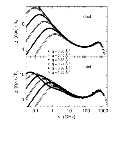
FIG. 8.: Dynamic susceptibility as in Fig. 6, rescaled with a $q$-dependent amplitude $h_{q}$ according to the factorisation (23). At small wavenumbers multiple scattering distorts in particular the intensity ratio of $\alpha$ relaxation vs fast relaxation. This can also be seen by comparing the amplitudes $A_{q}$ [Fig. 7] and $h_{q}$ [Fig. 10].

FIG. 9.: Rescaled susceptibility $\chi^{\prime\prime}(q,\nu)/h_{q}$ as in Fig. 8, but only for the largest wavenumbers $q=1.0\ldots 1.4$ Å^-1. The full curves are fits with the asymptotic scaling function $g_{\lambda}(\nu/\nu_{\sigma})$. Multiple-scattering causes a shift of the minimum position but has almost no influence on the line shape.

FIG. 10.: Amplitudes $h_{q}$ as used for the rescaling in Figs. 8 and 9. The wavenumber dependence is almost the same as for the low-frequency inelastic intensity in the glass model [Fig. 5]. The line indicates the transient linear $q$ dependence observed in several real experiments.

FIG. 11.: Distribution $f(2\theta^{\prime}|2\theta)$ of single-scattering angles $2\theta^{\prime}$ contributing to the elastic double-scattering for three different detector angles $2\theta$. From a simulation of the rigid model. The enhanced probability of $90^{\circ}$ scattering events is attributed to the sample geometry which admits long flight paths perpendicular to the scattering plane.

REFERENCES

- [1] U. Buchenau, N. Nücker and A. J. Dianoux, Phys. Rev. Lett. 53, 2316 (1984).
- [2] S. Cusack and W. Doster, Biophys. J. 58, 243 (1990).
- [3] J. Wuttke et al., Z. Phys. B 91, 357 (1993).
- [4] U. Buchenau, C. Pecharroman, R. Zorn and B. Frick, Phys. Rev. Lett. 77, 659 (1996).
- [5] M. Settles and W. Doster, in Biological Macromolecular Dynamics, edited by S. Cusack et al. (Proceedings of a Workshop on Inelastic and Quasielastic Neutron Scattering in Biology, Grenoble 1996), Adenine Press: Schenectady (1997).
- [6] M. Bée, Quasielastic Neutron Scattering, Hilger: Bristol (1988).
- [7] J. Wuttke et al., Phys. Rev. E 54, 5364 (1996).
- [8] R. Zorn, Phys. Rev. B 55, 6249 (1997).
- [9] W. Götze, in Liquids, Freezing and the Glass Transition, edited by J. P. Hansen, D. Levesque and D. Zinn-Justin (Les Houches, session LI), North Holland: Amsterdam (1991).
- [10] W. Götze and L. Sjögren, Rep. Progr. Phys. 55, 241 (1992).
- [11] W. Götze, Z. Phys. B 56, 139 (1984).
- [12] L. Sjögren, Phys. Rev. A 33, 1254 (1986).
- [13] Throughout this paper denotes the temperature-independent value .
- [14] W. Knaak, F. Mezei and B. Farago, Europhys. Lett. 7, 527 (1988).
- [15] W. Doster, S. Cusack and W. Petry, Phys. Rev. Lett. 65, 1080 (1990).
- [16] B. Frick, R. Zorn, D. Richter and B. Farago, J. Non-Cryst. Solids 131–133, 169 (1991).
- [17] J. Wuttke et al., Phys. Rev. Lett. 72, 3052 (1994).
- [18] J. Toulouse, R. Pick and C. Dreyfus, Mat. Res. Soc. Symp. Proc. 407, 161 (1996).
- [19] B. Rufflé et al., Phys. Rev. B 56, 11546 (1997).
- [20] A. Meyer et al., Phys. Rev. Lett. 80, 4454 (1998).
- [21] J. Wuttke et al., Eur. Phys. J. B 1, 169 (1998).
- [22] J. Wuttke et al., Phys. Rev. E 61, 2730 (2000).
- [23] A. P. Singh, Diplomarbeit, Technische Universität München (1995).
- [24] W. Götze, J. Stat. Phys. 83, 1183 (1996).
- [25] C. Alba-Simionescu and M. Krauzman, J. Chem. Phys. 102, 6574 (1995).
- [26] V. Krakoviack, C. Alba-Simionescu and M. Krauzman, J. Chem. Phys. 107, 3417 (1997).
- [27] T. Franosch, W. Götze, M. Mayr and A. P. Singh, Phys. Rev. E 55, 3183 (1997).
- [28] B. Rufflé, C. Ecolivet and B. Toudic, Europhys. Lett. 45, 591 (1999).
- [29] W. M. Du et al., Phys. Rev. E 49, 2192 (1994).
- [30] U. Schneider, P. Lunkenheimer, R. Brand and A. Loidl, Phys. Rev. E 59, 6924 (1999).
- [31] W. Götze and T. Voigtmann, Phys. Rev. E 61, 4133 (2000).
- [32] Parameter table kindly provided by T. Voigtmann.
- [33] For consistency with lower temperatures, the original fits of Ref. [31] also comprise a hopping term. With a strength hopping does not influence the dynamics at 220 K and will therefore be neglected.
- [34] It is an inherent weakness of the Sjögren model that the fourth condition for cannot be satisfied simultaneously.
- [35] F. G. Bischoff, M. L. Yeater and W. E. Moore, Nucl. Sci. Eng. 48, 266 (1972).
- [36] J. R. D. Copley, Comput. Phys. Comm. 7, 289 (1974).
- [37] J. R. D. Copley, P. Verkerk, A. A. van Well and A. Frederikze, Comput. Phys. Comm. 40, 337 (1986).
- [38] J. Wuttke, Physica B 266, 112 (1999).
- [39] J. Wuttke, Physica B (in press).
- [40] B. Frick, D. Richter, W. Petry and U. Buchenau, Z. Phys. B 70, 73 (1988).
- [41] M. Ferrand, A. J. Dianoux, W. Petry and G. Zaccai, Proc. Natl. Acad. Sci. USA 90, 9668 (1993).
- [42] B. Frick and D. Richter, Phys. Rev. B 47, 14795 (1993).
- [43] A. Mermet et al., Europhys. Lett. 38, 515 (1997).
- [44] This may explain (at least partially) the discrepancies shown in Fig. 2b of Ref. [22] where time-of-flight measurements with different incident wavelengths are compared.
- [45] M. Settles and W. Doster, Faraday Discuss. 103, 269 (1996).
- [46] M. Dishon, G. H. Weiss and J. T. Bendler, J. Res. N. B. S. 90, 27 (1985).
- [47] S. H. Chung and J. R. Stevens, Am. J. Phys. 59, 1024 (1991).
- [48] J. P. Boon and S. Yip, Molecular Hydrodynamics, McGraw Hill: New York (1980).
- [49] W. Götze, J. Phys. Condens. Matter 2, 8485 (1990).
- [50] M. Kiebel et al., Phys. Rev. B 45, 10301 (1992).
- [51] M. Goldammer and J. Wuttke, unpublished data on n-butyl-benzene and toluene.