Nature of phase transitions in a probabilistic cellular automaton with two absorbing states

Abstract

We present a probabilistic cellular automaton with two absorbing states, which can be considered a natural extension of the Domany-Kinzel model. Despite its simplicity, it shows a very rich phase diagram, with two second-order and one first-order transition lines that meet at a bicritical point. We study the phase transitions and the critical behavior of the model using mean field approximations, direct numerical simulations and field theory. The second-order critical curves and the kink critical dynamics are found to be in the directed percolation and parity conservation universality classes, respectively. The first order phase transition is put in evidence by examining the hysteresis cycle. We also study the “chaotic” phase, in which two replicas evolving with the same noise diverge, using mean field and numerical techniques. Finally, we show how the shape of the potential of the field-theoretic formulation of the problem can be obtained by direct numerical simulations.

1 Introduction

Probabilistic cellular automata (PCA) have been widely used to model a variety of systems with local interactions in physics, chemistry, biology and social sciences [1, 2, 3, 4, 5]. Moreover, PCA are simple and interesting models that can be used to investigate fundamental problems in statistical mechanics. Many classical equilibrium spin models can be reformulated as PCA, for example the kinetic Ising model with parallel heat-bath dynamics is strictly equivalent to a PCA with local parallel dynamics [6, 7]. On the other hand, PCA can be mapped to spin models [8] by expressing the transition probabilities as exponentials of a local energy. PCA can be used to investigate nonequilibrium phenomena, and in particular the problem of phase transitions in the presence of absorbing states. An absorbing state is represented by a set of configurations from which the system cannot escape, equivalent to an infinite energy well in the language of statistical mechanics. A global absorbing state can be originated by one or more local transition probabilities which take the value zero or one, corresponding to some infinite coupling in the local energy [8].

The Domany-Kinzel (DK) model is a boolean PCA on a tilted square lattice that has been extensively studied [9, 10]. Let us denote the two possible states of each site with the terms “empty” and “occupied”. In this model a site at time $t$ is connected to two sites at time $t-1$, constituting its neighborhood. The control parameters of the model are the local transition probabilities that give the probability of having an occupied site at a certain position once given the state of its neighborhood. The transition probabilities are symmetric for all permutations of the neighborhood, and this property is equivalent to saying that they depend on the sum of “occupied” sites in the neighborhood, whence the term “totalistic” used to denote this class of automata.

In the DK model the transition probability from an empty neighborhood to an occupied state is zero, thus the empty configuration is an absorbing state. For small values of the other transition probabilities, any initial configuration will evolve to the absorbing state. For larger values, a phase transition to an active phase, represented by an ensemble of partially occupied configurations, is found. The order parameter of this transition is the asymptotic average fraction of occupied sites, which we call the density. The critical properties of this phase transition belong to the directed percolation (DP) universality class (except for one extreme point) [11], and the DK model is often considered the prototype of such a class.

The evolution of this kind of models is the discrete equivalent of the trajectory of a stochastic dynamical system. One can determine the sensitivity with respect to a perturbation, by studying the trajectories originating by two initially different configurations (replicas) evolving with the same realization of the stochasticity, e.g. using the same sequence of random numbers. The order parameter here is the asymptotic difference between the two replicas, which we call the damage. It turns out that, inside the active phase, there is a “chaotic” phase in which the trajectories depend on the initial configurations and the damage is different from zero, and a non chaotic one in which all trajectories eventually synchronize with the vanishing of the damage. In simple models like the DK one, this transition does not depend on the choice of the initial configurations (provided they are different from the absorbing state) and the initial damage [12].

It has been conjectured that all second-order phase transitions from an “active” phase to a non degenerate, quiescent phase (generally represented by an absorbing state) belong to the DP universality class if the order parameter is a scalar and there are no extra symmetries or conservation laws [14, 15]. This has been verified in a wide class of models, even multi-component, and in the presence of several asymmetric absorbing states [16]. Also the damage phase transition has a similar structure. Once synchronized, the two replicas cannot separate, and thus the synchronized state is absorbing. Indeed, numerical simulations shows that it is in the DP universality class [13]. Moreover, in the DK model, the damage phase transition can be mapped onto the density one [7].

On the other hand, some models with conserved quantities [17, 18] or symmetric absorbing states belong to a different universality class called parity conservation (PC) or directed Ising [19, 20]. This universality class appears to be less robust since it is strictly related to the symmetry of the absorbing states; a slight asymmetry is sufficient to bring the model to the usual DP class [19, 20].

An interesting question concerns the simplest, one-dimensional PCA model with short range interactions exhibiting a first order phase transition. Dickman and Tomé [21, 22] proposed a contact process with spontaneous annihilation, auto catalytic creation by trimers and hopping. They found a first order transition for high hopping probability, i.e., in the region more similar to mean field (weaker spatial correlations).

Bassler and Browne discussed a model whose phase diagram also presents first and second-order phase transitions [30]. In it, monomers of three different chemical species can be adsorbed on a one-dimensional surface and neighboring monomers belonging to different species annihilate instantaneously. The control parameters of the model are the absorption rates of the monomers. The transition from a saturate to a reactive phase belongs to the DP universality class, while the transition between two saturated phases is discontinuous. The point at which three phase transition lines join does belong to the PC universality class.

Scaling and fluctuations near first order phase transitions are also an interesting subject of study [23, 24, 25, 26], which can profit from the existence of simple models.

In this paper we study a one-dimensional, one-component, totalistic PCA with two absorbing states. It can be considered as a natural extension of the DK model to a lattice in which the neighborhood of a site at time $t$ contains the site itself and its two nearest neighbors at time $t-1$. This space-time lattice arises naturally in the discretization of one-dimensional reaction-diffusion systems. In our model, the transition probabilities from an empty neighborhood is zero, and that from a completely occupied neighborhood is one. The model has two absorbing states: the completely empty and the completely occupied configurations. The order parameter is again the density; it is zero or one in the two quiescent phases, and assumes other values in the active phase. The system presents a line of symmetry in the phase diagram, over which the two absorbing phases have the same importance. A more detailed illustration of the model can be found in Section 2.

This model can arise as a particular case of a nonequilibrium wetting of a surface. In this framework, only a single layer of particles can be absorbed on the surface. If we assume that particles can be absorbed or desorbed only near the boundaries of a patch of already absorbed particles (when the neighborhood is not homogeneous), then the completely empty and occupied configurations are absorbing states.

This totalistic PCA can also be interpreted as a simple model of opinion formation. It assumes that an individual may change his mind according to himself and his two nearest neighbors. The role of social pressure is twofold. If there is homogeneity of opinions, individuals cannot disagree (absorbing states), otherwise they can agree or disagree with the majority with a certain probability.

The density phase diagram shows two second order phase transition curves separating the quiescent phases from the active one, and a first order transition line between the two quiescent phases, as discussed in Section 3. These curves meet on the line of symmetry in a bicritical point. We use both mean field approximations and direct numerical simulations. The former simple approximation gives a qualitatively correct phase diagram. The numerical experiments are partially based on the fragment method [31]. This is a parallel algorithm that implements directly the evolution rule for different values of the control parameters on the bits of one or more computer words.

In Section 4, we investigate numerically the second order phase transitions and find they belong to the DP universality class. Along the line of symmetry of the model the two absorbing phases are equivalent. In Appendix B we show that on this line one can reformulate the problem in terms of the dynamics of kinks between patches of empty and occupied sites. Since the kinks are created and annihilated in pairs, the dynamics conserves the initial number of kinks modulo two. In this way we can present an exact mapping between a model with symmetric absorbing phases and one with parity conservation. We find that the critical kink dynamics at the bicritical point belongs to the PC universality class.

In Section 5 we study the chaotic phase, using dynamic mean field techniques (reported in Appendix  A) and direct numerical simulations. The location of this phase is similar to that of the DK model: it joins the second-order critical curves at the boundary of the phase diagram.

Our model exhibits a first-order phase transition along the line of symmetry in the upper part of the phase diagram. A first-order transition is usually associated to an hysteresis cycle. It is possible to observe such a phenomena by adding a small perturbing field to the absorbing states, as discussed in Section 6.

The DP universality class is equivalent to the Reggeon field theory [27], which in $d=0$ corresponds to a quadratic potential with a logarithmic divergence at the origin. The Langevin description for systems in the PC class yields a similar potential, except for irrelevant terms [18]. It has been shown [28] that one can reconstruct the potential from the numerical integration of the Langevin equation, which, however, requires special techniques in the presence of absorbing states [29]. In Section 7 we show how the potential is reconstructed from actual simulations of a phenomenological model, such as our original cellular automata or the kink dynamics. In this way we obtain the shape of the potential for a system in the parity conservation universality class.

2 The model

We describe here a one-dimensional, totalistic, probabilistic cellular automaton with three inputs. The state of the model at time $t$ is given by $\boldsymbol{x}^{t}=(x_{0}^{t},\dots,x_{L-1}^{t})$ with $x_{i}^{t}\in\{0,1\}$; $t=1,2,\dots$ and $L$ is the number of sites. All operations on spatial indices are assumed to be modulo $L$ (periodic boundary conditions). For simplicity of notation, we write $x=x_{i}^{t}$, $x_{-}=x_{i-1}^{t}$, $x_{+}=x_{i+1}^{t}$ and $x^{\prime}=x_{i}^{t+1}$. We shall indicate by $\sigma=x_{-}+x+x_{+}$ number of occupied cells in the neighborhood. The most general three-input totalistic PCA is defined by the quantities $p_{s}$, which are the conditional probabilities that $x^{\prime}=1$ if $\sigma=s$. The microscopic dynamics of the model is completely specified by

$$x^{\prime}=\sum_{s=0}^{3}R_{s}\delta_{\sigma,s}.$$ (1)

In this expression $R_{s}$ is a stochastic binary variable that takes the value 1 with probability $p_{s}$ and 0 with probability $1-p_{s}$, and $\delta$ is the Kronecker delta. In practice, we implement $R_{s}$ by extracting a random number $r_{s}$ uniformly distributed between 0 and 1, and setting $R_{s}$ equal to 1 if $r_{s}<p_{s}$ and 0 otherwise. Eq. (1) implies the use of four random numbers $r_{s}$ for each site. The evolution of a single trajectory is not affected by the eventual correlations among the $r_{s}$, since only one $\delta_{\sigma,s}$ is different from zero. This is not true when computing the simultaneous evolution of two or more replicas using the same noise. If not otherwise stated, we use only one random number for all the $r_{s}$. More discussions about the choice of random numbers can be found in Section 5 and in Appendix B.

With $p_{0}=0$ and $p_{3}=1$ the model presents two quiescent phases: the phase 0 corresponding to the configuration $x=(0,\dots,0)$ and the phase 1 corresponding to the configuration $x=(1,\dots,1)$. In this case there are two control parameters, $p_{1}$ and $p_{2}$, and the model is symmetric under the changes $p_{1}\to 1-p_{2}$, $p_{2}\to 1-p_{1}$ and $x\to x\oplus 1$ where $\oplus$ is the exclusive disjunction (or the sum modulo 2).

3 Phase diagram

Figure 1: Mean-field phase diagram for the density $c$ of active sites. The white (black) region corresponds to the phase 0 (phase 1). The levels of grey indicate different values of the asymptotic density $c$ (active phase), the lightest corresponds to $0<c<1/4$, and the next ones to $1/4<c<1/2$, $1/2<c<3/4$ and $3/4<c<1$. The two quiescent phases coexist in the hatched region.

In order to have a qualitative idea of the behavior of the model, we first study the mean-field approximation. If $c$ and $c^{\prime}$ denote the density of occupied sites at times $t$ and $t+1$ respectively,

$$\begin{split}c^{\prime}&=3p_{1}c\left(1-c\right)^{2}+3p_{2}c^{2}\left(1-c\right)+c^{3}.\end{split}$$ (2)

This map has three fixed points, $c_{0}$, $c_{1}$, and $c_{2}$ given by

$$c_{0}=0,\quad c_{1}=\frac{3p_{1}-1}{1+3p_{1}-3p_{2}},\quad\hbox{and}\quad c_{2}=1.$$

The asymptotic density will assume one of the latter values according to the values of the control parameters and the initial state as we show in Fig. 1. In the square $1/3<p_{1}\leq 1$, $0\leq p_{2}<2/3$, the only stable fixed point is $c_{1}$. Inside this square, on the segments $p_{2}-2/3=m(p_{1}-1/3)$ with $m<0$, $c_{1}=1/(1-m)$.The first fixed point $c_{0}$ is stable when $p_{1}<1/3$ and $c_{2}$ is stable when $p_{2}>2/3$. There is a continuous second-order transition from the quiescent phase 0 to the active phase on the segment $p_{1}=1/3$, $0\leq p_{2}<2/3$ and another continuous transition from the active to the quiescent phase 1 on the segment $1/3<p_{1}\leq 1,p_{2}=2/3$.

In the hatched region of Fig. 1 $c_{0}$ and $c_{2}$ are both stable. Their basins of attraction are, respectively, the semi-open intervals $[0,c_{1})$ and $(c_{1},1]$. Starting from a uniformly distributed random value of $c$, as time $t$ goes to infinity, $c$ tends to $c_{0}$ with probability $c_{1}$, and to $c_{2}$ with probability $1-c_{1}$. Since, for $p_{1}+p_{2}=1$, $c_{1}=1/2$, the segment $p_{1}+p_{2}=1$, with $0\leq p_{1}<1/3$ and $2/3<p_{2}\leq 1$, is similar to a first-order transition line between the phase 0 and the phase 1.

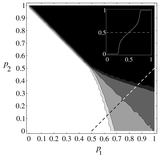
Figure 2: Phase diagram for the density of active sites $c$ by numerical experiments. One run was performed with $L=10000$ and $T=10000$. The graph shows $64\times 64$ values of $p_{1}$ and $p_{2}$. The color code is the same as in Fig. 1. The inset represents the density profile along the dashed line. Two critical phase transitions are evident.

In Fig. 2 we show the phase diagram of the model obtained numerically starting from a random initial state with half of the cells occupied. The scenario is qualitatively the same as predicted by the mean-field analysis. In the vicinity of the point $(p_{1},p_{2})=(0,1)$ we observe a discontinuous transition from $c=0$ to $c=1$. The two second-order phase-transition curves from the active phase to the quiescent phases are symmetric, and the critical behavior of the order parameter, $c$ for the lower curve and $1-c$ for the upper one, is the same.

Due to the symmetry of the model the two second-order phase transition curves meet at a bicritical point $(p_{t},1-p_{t})$ where the first-order phase transition line $p_{1}+p_{2}=1$, $p_{1}<p_{t}$ ends. Crossing the second-order phase boundaries on a line parallel to the diagonal $p_{1}=p_{2}$, the density $c$ exhibits two critical transitions, as shown in the inset of Fig. 2. Approaching the bicritical point the critical region becomes smaller, and corrections to scaling increase. Finally, at the transition point the two transitions coalesce into a single discontinuous one.

4 Critical dynamics and universality classes

We performed standard dynamic Monte Carlo simulations starting from a single site in the origin out of the nearest absorbing state, and measured the average number of active sites $N(t)$, the survival probability $P(t)$ and the average square distance from origin $R^{2}(t)$ (averaged over surviving runs) defined as

$$\begin{split}N(t)&=\dfrac{1}{K}\sum_{k=1}^{K}\sum_{i}\omega_{i}^{t}(k),\\ P(t)&=\dfrac{1}{K}\sum_{k=1}^{K}\theta\left(\sum_{i}\omega_{i}^{t}(k)\right),\\ R^{2}(t)&=\dfrac{1}{KN(t)}\sum_{k=1}^{K}\sum_{i}\omega_{i}^{t}(k)i^{2}.\end{split}$$ (3)

In these expressions, $k$ labels the different runs and $K$ is the total number of runs. The quantity $\omega_{i}$ is $x_{i}$ if the nearest absorbing state is $\boldsymbol{0}$ and $1-x_{i}$ otherwise; $\theta$ is the Heaviside step function, that assumes the value 1 if its argument is greater than 0, and the value 0 if it is smaller than 0.

At the critical point one has

$$N(t)\sim t^{\eta},\quad P(t)\sim t^{-\delta},\quad R^{2}(t)\sim t^{z}.$$

At the transition point $(p^{*}_{1}=0.6625(3),p_{2}=0)$, we get $\eta=0.308(5)$, $\delta=0.160(2)$ and $z=1.265(5)$, in agreement with the best known values for the directed percolation universality class [32].

Near the bicritical point, on the line $p_{1}+p_{2}=1$, the two absorbing states have symmetrical weight. We define a kink $y_{i}$ as $y_{i}=x_{i}\oplus x_{i+1}$. For the computation of the critical properties of the kink dynamics, one has to replace $\omega_{i}$ with $y_{i}$ in Eq. (3). The evolution equation is derived in Appendix B. In the kink dynamics there is only one absorbing state (the empty state), corresponding to one of the two absorbing states $\boldsymbol{0}$ or $\boldsymbol{1}$. For $p_{1}<p_{t}$ the asymptotic value of the density of kinks is zero and it starts to grow for $p_{1}>p_{t}$. In models with multiple absorbing states, dynamical exponents may vary with initial conditions. Quantities computed only on survival runs ($R^{2}(t)$) appear to be universal, while others (namely $P(t)$ and $N(t)$) are not [33].

We performed dynamic Monte Carlo simulations starting either from one and two kinks. In both cases $p_{t}=0.460(2)$, but the exponents were found to be different. Due to the conservation of the number of kinks modulo two, starting from a single site one cannot observe the relaxation to the absorbing state, and thus $\delta=0$. In this case $\eta=0.292(5)$, $z=1.153(5)$. On the other hand, starting with two neighboring kinks, we find $\eta=0.00(2)$, $\delta=0.285(5)$, and $z=1.18(2)$. These results are consistent with those found by other authors [17, 18, 19].

5 The chaotic phase

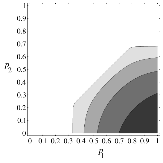
Figure 3: Mean-field damage-spreading phase diagram. The diagram has been obtained numerically iterating Eq. (A.1). The lightest level of grey corresponds to $0<h<1/8$, the next ones to $1/8<h<1/4$, $1/4<h<3/8$ and $3/8<h<1/2$ respectively.

Let us now turn to the sensitivity of the model to a variation in the initial configuration, i.e. to the study of damage spreading or, equivalently, to the location of the chaotic phase.

Given two replicas $x$ and $y$, we define the difference $w$ as $w=x\oplus y$. The damage $h$ is defined as the fraction of sites in which $w=1$, i.e. as the Hamming distance between the configurations $x$ and $y$.

The precise location of this phase transition depends on the particular implementation of the stochasticity. Since the sum of occupied cells in the neighborhood of $x$ is in general different from that of $y$, the evolution equation (1) for the two replicas uses different random numbers $r_{s}$. The correlations among these random numbers affect the location of the chaotic phase boundary [34].

We limit our investigation to the case of maximal correlations by using just one random number per site, i.e. all $r_{s}$ are the same for all $s$ at the same site. This gives the smallest possible chaotic region. Notice that we have to extract a random number for all sites, even if in one or both replicas have a neighborhood configuration for which the evolution rule is deterministic (if $\sigma=0$ or $\sigma=3$).

One can write the mean field equation for the damage by taking into account all the possible local configurations of two lattices. The evolution equation for the damage depends on the correlations among sites but in the simplest case we can assume that $h(t+1)$ depends only on $h(t)$ and $c(t)$, the density of occupied sites. In Appendix A we find the evolution equation for the damage in the mean-field approximation. In Fig. 3 we show the phase diagram of the chaotic phase in this approximation. There is a qualitative agreement with the mean field phase diagram found for the DK model [35].

Figure 4: Phase diagram for the damage spreading from direct numerical simulations. The color code is that of Fig. 3 Traces of the second order phase transitions are present; they join to the first-order ($c_{0}=0.5$) phase boundary.

In Fig. 4 we show the phase diagram for the damage found numerically by considering the evolution starting from uncorrelated configurations with initial density equal to 0.5. The damage region is shown in shades of grey. Outside this region there appear small damaged domains on the other phase boundaries. This is due either to the divergence of the relaxation time (second-order transitions) or to the fact that a small difference in the initial configuration can drive the system to a different absorbing state (first-order transitions). The chaotic domain near the point $(p_{1},p_{2})=(1,0)$ is stable regardless of the initial density. On the line $p_{2}=0$ the critical points of the density and the damage coincide at $p^{*}_{1}$.

6 First-order phase transition and hysteresis cycle

First-order phase transitions are usually associated to a hysteresis cycle due to the coexistence of two phases. In the absence of absorbing states, the coexistence of two stable phases for the same values of the parameters is a transient effect in finite systems, due to the presence of fluctuations. To find the hysteresis loop we modify the model slightly by putting $p_{0}=1-p_{3}=\varepsilon$ with $\varepsilon\ll 1$. In this way the empty and fully occupied configurations are no longer absorbing. This brings the model back into the class of equilibrium models for which there is no phase transition in one dimension but metastable states can nevertheless persist for long times. The mean field equation for the density $c$ becomes

$$\begin{split}c^{\prime}=&\varepsilon(1-c)^{3}+3p_{1}c\left(1-c\right)^{2}+\\ &3p_{2}c^{2}\left(1-c\right)+(1-\varepsilon)c^{3}.\end{split}$$ (4)

We study the asymptotic density as $p_{1}$ and $p_{2}$ move on a line with slope 1 inside the hatched region of Fig. 1. For $p_{1}$ close to zero, Eq. (4) has only one fixed point, which is stable and close to $\varepsilon$. As $p_{1}$ increases adiabatically (by taking $c$ at $t=0$ equal the previous value of the fixed point) the new asymptotic density will still assume this value even when two more fixed points appear one of which is unstable and the other stable and close to one. Eventually the first fixed point disappears, and the asymptotic density jumps to the stable fixed point close to one. Going backwards on the same line, the asymptotic density will be close to one until that fixed point disappears and it will jump back to a small value close to zero. By symmetry, the hysteresis loop is centered around the line $p_{1}+p_{2}=1$ which we identify as a first-order phase transition line inside the hatched region.

Figure 5: Profile of the hysteresis region for several values of the noise $\varepsilon$ and relaxation time $T$ according to the local structure approximation with $l=6$. The curves represent the intersections of the hysteresis cycle with $c=0.5$ (horizontal dashed line in the inset). The curves join smoothly at $p_{1}=0$, $p_{2}=1$ (not represented). Starting from the out most curve, these correspond to $T=500$, $\varepsilon=0.0001$; $T=1000$, $\varepsilon=0.0001$, and $T=500$, $\varepsilon=0.001$. The dashed lines represent the mean-field hysteresis region. The inset represents the cycle along a line parallel to the diagonal $p_{1}=p_{2}$.

The hysteresis region is found by two methods, the dynamical mean field, which extends the mean field approximation to blocks of $l$ sites [36], and direct numerical experiments. As stated before it is necessary to introduce a small perturbation $\varepsilon=p_{0}=1-p_{3}$. We consider lines parallel to the diagonal $p_{1}=p_{2}$ in the parameter space and increase the value of $p_{1}$ and $p_{2}$ after a given relaxation time $t_{r}$ up to $p_{2}=1$; afterwards the scanning is reverted down to $p_{1}=0$. The hysteresis region for various values of parameters are reported Fig. 5. In numerical simulations, one can estimate the size of the hysteresis region by starting with configurations $\boldsymbol{0}$ and $\boldsymbol{1}$, and measuring the size $d$ of the region in which the two simulations disagree.

7 Reconstruction of the potential

Figure 6: Reconstruction of potential $V(c)$ for $p_{2}=0$. We performed $10^{4}$ runs over a system of 500 sites and computed the probability distribution $P(n)$ averaging over 500 time steps after discarding 1000 time steps. We limited to small times in order to be able to see the divergence at the origin (the absorbing state) together with the other local minimum (the active state).

Figure 7: Reconstruction of potential $V(c)$ for the kink dynamics on the line $p_{2}=1-p_{1}$. The simulations were carried out as described in the previous figure caption.

An important point in the study of systems exhibiting absorbing states is the formulation of a coarse-grained description using a Langevin equation. It is generally accepted that DP universal behavior is represented by

$$\dfrac{\partial c(x,t)}{\partial t}=ac(x,t)-bc^{2}(x,t)+\nabla^{2}c(x,t)+\sqrt{c(x,t)}\alpha(x,t),$$ (5)

where $c$ is the density field, $a$ and $b$ are control parameters and $\alpha$ is a Gaussian noise with correlations $\langle\alpha(x,t)\alpha(x^{\prime},t^{\prime})\rangle=\delta_{x,x^{\prime}}\delta_{t,t^{\prime}}$. The diffusion coefficient has been absorbed into the parameters $a$ and $b$ and the time scale. This equation can be obtained by a mean-field approximation of the evolution equation keeping only the relevant terms. The state $c(x,t)=0$ is clearly stationary, but its absorbing character is given by the balance between fluctuations, which are of order of the field itself, and the “potential” part $ac-bc^{2}$ (See also Ref. [28]).

The role of the absorbing state can be illustrated by taking a sequence of equilibrium models whose energy landscape exhibits the coexistence of an infinitely deep well (the absorbing state) and another broad local minimum (corresponding to the “active”, disordered state), separated by an energy barrier. There is no true stationary active state for such a system (with a finite energy barrier), since there is always a probability of jumping into the absorbing state. However, the system can survive in a metastable active state for time intervals of the order of the inverse of the heigth of the energy barrier. The parameters controlling the height of the energy barrier are the size of the lattice and the length of the simulation: the equilibrium systems are two-dimensional with asymmetric interactions in the time direction [8]. In the limiting case of an infinite system, the height of the energy barrier is finite below the transition point, and infinite above, when the only physically relevant state is the disordered one.

It is possible to introduce a zero-dimensional approximation to the model by averaging over the time and the space, assuming that the system has entered the metastable state. In this approximation, the size of the original systems enters through the renormalized coefficients $\overline{a}$, $\overline{b}$,

$$\dfrac{\partial c(x,t)}{\partial t}=\overline{a}c(x,t)-\overline{b}c^{2}(x,t)+\sqrt{c(x,t)}\alpha(x,t),$$

where also the time scale has been renormalized.

The associated Fokker-Planck equation is

$$\dfrac{\partial P(c,t)}{\partial t}=-\dfrac{\partial}{\partial c}(\overline{a}c-\overline{b}c^{2})P(c,t)+\dfrac{1}{2}\dfrac{\partial^{2}}{\partial c^{2}}cP(c,t),$$

where $P(c,t)$ is the probability of observing a density $c$ at time $t$. One possible solution is a $\delta$-peak centered at the origin, corresponding to the absorbing state.

By considering only those trajectories that do not enter the absorbing state during the observation time, one can impose a detailed balance condition, whose effective agreement with the actual probability distribution has to be checked a posteriori.

A stationary distribution $P(c)=\exp(-V(c))$ corresponds to an effective potential $V(c)$ of the form

$$V(c)=\log(c)-2\overline{a}c+\overline{b}c^{2}.$$

Note that this distribution is not normalizable. One can impose a cutoff for low $c$, making $P(c)$ normalizable. For finite systems the only stationary solution is the absorbing state. However, by increasing the size of the system, one approximates the limit in which the energy barrier is infinitely hight, the absorbing state unreachable and $P(c)$ is the observable distribution.

In order to find the form of the effective potential for spatially extended systems, Muñoz [28] numerically integrated Eq. (5), using the procedure described by Dickman [29]. It is however possible to obtain the shape of the effective potential from the actual simulations, simply by plotting $V(c)=-\log(P(c))$ versus $c$, where $c$ is the density of the configuration.

In Fig. 6 we show the profile of the reconstructed potential $V$ for some values of $p$ around the critical value or the infinite system $p^{*}_{1}$ on the line $q=0$. We used rather small systems and followed the evolution for a limited amount of time in order to balance the weight of the $\delta$-peak with respect to $P(c)$ (which is only metastable). For larger systems the absorbing state is not visible above the transition and dominates below it.

On the line $q=0$ the model belongs to the DP universality class. One can observe that the curve becomes broader in the vicinity of the critical point, in correspondence of the divergence of critical fluctuations $\chi\sim|p-p_{c}|^{-\gamma^{\prime}}$, $\gamma^{\prime}=0.54$ [32]. By repeating the same type of simulations for the kink dynamics (random initial condition), we obtain slightly different curves, as shown in Fig. 7. We notice that all curves have roughly the same width. Indeed, the exponent $\gamma^{\prime}$ for systems in the PC universality class is believed to be exactly 0 [33], as given by the scaling relation [32] $\gamma^{\prime}=d\nu_{\perp}-2\beta$. Clearly, much more informations can be obtained from the knowledge of $P(c)$, either by direct numerical simulations or dynamical mean field trough finite scale analysis, as shown for instance in Ref. [37].

8 Discussions and conclusions

We have studied a probabilistic cellular automata with two absorbing states and two control parameters. This is a simple and natural extension of the Domany-Kinzel (DK) model. Despite its simplicity it has a rich phase diagram with two symmetric second-order phase curves that join a first-order line at a bicritical point. The phase diagram and the critical properties of the model were found using several mean field approximations and numerical simulations. The second-order phase transitions belong to the directed percolation universality class except for the bicritical point, which belongs to the parity conservation (PC) universality class. The first-order phase transition line was put in evidence by a modification of the model that allows one to find the hysteresis cycles. The model also presents a chaotic phase analogous to the one present in the DK model. This phase was studied using direct numerical simulations and dynamical mean field.

On the line of symmetry of the model the relevant behavior is given by kink dynamics. We found a closed expression for the kink evolution rule and studied its critical properties, which belong to the PC universality class. The effective potential governing the coarse-grained evolution for the DP and the PC phase was found through direct simulations, confirming that critical fluctuations diverge at most logarithmically in the PC class.

The phase diagram of our model is qualitatively similar to Bassler and Browne’s (BB) one [30]. In both models two critical lines in the DP universality class meet at a bicritical point in the PC universality class, and give origin to a first-order transition line. This suggests that the observed behavior has a certain degree of universality.

An interesting feature of the BB model is that the absorbing states at the bicritical point are indeed symmetric, but the model does not show any conserved quantities. We have shown that the bicritical dynamics of our model can be exactly formulated either in terms of symmetric states or of kinks dynamics, providing an exact correspondence between the presence of conserved quantities and the symmetry of absorbing states.

Furthermore, in order to obtain a qualitatively correct mean-field phase diagram of the BB model, one has to include correlations between triplets, while the mean-field phase diagram of our model is already correct at first approximation. This suggests that we have described a simpler model, which can be used as prototype for multi-critical systems.

Appendix A Damage spreading in the mean field approximation

The minimum damage spreading occurs when the two replicas $\boldsymbol{x}$ and $\boldsymbol{y}$ evolve using maximally correlated random numbers, i.e. when all $r_{s}$ in Eq. (1) are the same. [34]. Let $w=x\oplus y$ be the damage at a site $i$ and time $t$. It is also possible to consider $w$ as an independent variable and write $y=x\oplus w$. We denote $s=x_{-}+x+x_{+}$, $s^{\prime}=y_{-}+y+y+=(x_{-}\oplus w_{-})+(x\oplus w)+(x_{+}\oplus w_{+})$ and $s^{\prime\prime}=w_{-}+w+w_{+}$. The evolution equation for $h$, the density of damaged sites $w$ at time $t$, is obtained by considering all the local configurations $x_{-}xx_{+}$ and $w_{-}ww_{+}$ of one replica and of the damage

$$h^{\prime}=\sum_{\begin{subarray}{c}{x_{-}xx_{+}}\\ {w_{-}ww_{+}}\end{subarray}}\pi(c,s,3)\pi(h,s^{\prime\prime},3)\big{|}p_{s}-p_{s^{\prime}}\big{|},$$ (A.1)

where

$$\pi(\alpha,n,m)=\alpha^{n}(1-\alpha)^{n-m}.$$

In this equation all the sums run from zero to one. The value of $c$ is given by Eq. (2). The term $|p_{s}-p_{s^{\prime}}|$ is the probability that $R_{s}\oplus R_{s^{\prime}}$ is one using only one random number for the $r_{s}$. The argument of the sum is the probability that $x^{\prime}\neq y^{\prime}$. It is possible to rewrite Eq.(A.1) in a different form

$$h^{\prime}=\sum_{ss^{\prime}\ell}\binom{m}{s}\binom{m-s}{\ell}\binom{m-s}{s^{\prime}-\ell}\pi(c,s,m)\pi(\eta,s+s^{\prime}-2\ell,m)\lvert p_{s}-p_{s^{\prime}}\rvert,$$ (A.2)

where $s$ and $s^{\prime}$ are the same as above, and $\ell$ is the overlap between $x$ and $y$, i.e. $\ell=(x_{-}\wedge y_{-})+(x\wedge y)+(x_{+}\wedge y_{+})$ ($\wedge$ is the AND operation). Assuming that $\binom{a}{b}=0$ if $b>a$, $a<0$ or $b<0$, the sum of (A.2) can run over all positive integers. This expression is valid for all totalistic rules with a neighborhood of size $m$ (here $m=3$).

The stationary state of Eq. (A.1) (or Eq. (A.2)) can be found analytically using a symbolic manipulation program. The chaotic transition line is

$$p_{2}=p_{1}-\dfrac{1}{9},$$

with $1/3<p_{1}<1$,$0<p_{2}<2/3$.

Appendix B Kink dynamics

On the segment $p_{1}+p_{2}=1$, $p_{1}<p_{t}$ the order parameter is the number of kinks. The dynamics of the kinks $y_{i}=x_{i}\oplus x_{i+1}$ (that for the ease of notation we write $y=x\oplus x_{+}$) is obtained by taking the exclusive disjunction of $x^{\prime}=x_{i}^{t+1}$ and $x^{\prime}_{+}=x_{i+1}^{t+1}$ given by Eq. (1). In order to obtain a closed expression for the $y$, a little of Boolean algebra is needed.

The totalistic functions $\delta_{\sigma,s}$ where $s=x_{-}+x+x_{+}$ can be expressed in terms of the symmetric polynomials $\xi^{(j)}$ of degree $j$ [38]. These are

$$\begin{split}\xi^{(1)}&=x_{-}\oplus x\oplus x_{+},\\ \xi^{(2)}&=x_{-}x\oplus x_{-}x_{+}\oplus xx_{+},\\ \xi^{(3)}&=\xi^{(1)}\xi^{(2)}=x_{-}xx_{+}.\end{split}$$

The totalistic functions are given by

$$\begin{split}\delta_{\sigma,1}&=\xi^{(1)}\oplus\xi^{(3)},\\ \delta_{\sigma,2}&=\xi^{(2)}\oplus\xi^{(3)},\\ \delta_{\sigma,3}&=\xi^{(3)}.\end{split}$$

In the evolution equation (1), one has $R_{1}=1$ if $r_{1}<p_{1}$, and $R_{2}=1$ if $r_{2}<p_{2}$. On the line $p_{1}+p_{2}=1$ (i.e. $p_{2}=1-p_{1}$), $R_{2}$ takes the value 1 if $1-r_{2}>p_{1}$. Choosing $1-r_{2}=r_{1}$ (this choice does not affect the dynamics of a single replica) we have $R_{2}=R_{1}\oplus 1$ and Eq. (1) becomes, after some manipulations,

$$x^{\prime}=R(\xi^{(1)}\oplus\xi^{(2)})\oplus\xi^{(2)},$$

where $R=R_{1}$. One can easily check that

$$\xi^{(1)}=y_{-}\oplus y\oplus x,$$

and

$$\xi^{(2)}=y_{-}y\oplus x.$$

Finally, we obtain the evolution equation for the $y$

$$\begin{split}y^{\prime}&=x^{\prime}\oplus x^{\prime}_{+}\\ &=R(y_{-}\oplus y\oplus y_{-}y)\oplus R_{+}(y\oplus y_{+}\oplus yy_{+})\oplus y_{-}y\oplus yy_{+}\oplus y\\ &=R(y_{-}\vee y)\oplus R_{+}(y\vee y_{+})\oplus y_{-}y\oplus yy_{+}\oplus y,\end{split}$$ (B.3)

In this expression $\vee$ denotes the disjunction operation (OR). The sum modulo 2 (XOR) of all $y_{i}$ over the lattice is invariant with time, since all repeated terms cancel out ($a\oplus a=0$). Note that the kink dynamics uses correlated noise between neighboring sites.

References

- [1] D. Farmer, T. Toffoli, and S. Wolfram, editors, Cellular Automata, (Los Alamos Interdisciplinary Workshop), North Holland, Amsterdam, 1984.
- [2] S. Wolfram, editor, Theory and Applications of Cellular Automata, World Scientific, Singapore, 1987.
- [3] P. Manneville, N. Boccara, G. Vichniac, and R. Bidaux, editors, Cellular Automata and Modeling of Complex Physical Systems, (Les Houches Workshop), Springer, Heidelberg, 1989.
- [4] H. Gutowitz, editor, Cellular Automata: Theory and Experiments, (Los Alamos Workshop), North-Holland, Amsterdam, 1990.
- [5] N. Boccara, E. Goles, S. Martínez, and P. Picco, editors, Cellular Automata and Cooperative Phenomena, (Les Houches Workshop), Kluwer, 1993.
- [6] F. Bagnoli, R. Rechtman and S. Ruffo, J. Comp. Phys 101 763 (1991).
- [7] F. Bagnoli, J. Stat. Phys. 85, 151 (1996).
- [8] A. Georges and P. Le Doussal, J. Stat. Phys. 54, 1011 (1989).
- [9] E. Kinzel and W. Domany, Phys. Rev. Lett. 53 (1984).
- [10] W. Kinzel, Z. Phys. B 58 (1985).
- [11] W. Kinzel, in Percolation Structures and Processes, G. Deutsch, R. Zallen and J. Adler, editors (Adam Hilger, Bristol, 1983).
- [12] M. L. Martins, H. F. Verona de Resende, C. Tsallis, A. C. N. de Magalhães, Phys. Rev. Lett. 66, 2045 (1991).
- [13] P. GRassberger, J. Stat. Phys. 79, 13 (1985).
- [14] H. K. Janssen, Z. Phys. B 42, 152 (1981).
- [15] P. Grassberger, Z. Phys. B 47, 365 (1982).
- [16] See references in [19].
- [17] P. Grassberger, F. K. F, and T. von der Twer, J. Phys. A: Math. Gen. 17, L105 (1984).
- [18] P. Grassberger, J. Phys. A: Math. Gen. 22, L1103 (1989).
- [19] H. Hinrichsen, Phys. Rev. E 55, 219 (1997); cond-mat/9608065 (1996).
- [20] W. Hwang, A. Kwon, H. Park and H. Park, Phys. Rev. E 57, 6438 (1998).
- [21] R. Dickman and T. Tomé, Phys. Rev. A 44 4833 (1991).
- [22] R. Dickman and J. Marro, Nonequilibrium phase transitions in lattice models (Cambridge University Press, Cambridge, 1999).
- [23] M. Ehsasi et al., J. Chem. Phys. 91, 4949 (1989).
- [24] J. W. Evans and M. S. Miesch, Phys. Rev. Lett. 66, 833 (1991) and Surf. Sci. 245, 401 (1991); J. W. Evans and T. R. Ray, Phys. Rev. E., 50, 4302 (1994).
- [25] R.A. Monetti, A. Rozenfeld and E.V. Albano, First-order phase transitions in nonequilibrium systems: New perspectives, cond-mat/9911040 (1999).
- [26] H. Hinrichsen, R. Livi, D. Mukamel and A. Politi, First-order phase transition in a -dimensional nonequilibrium wetting phase, cond-mat/9906039 (1999)
- [27] J. L. Cardy, R. L. Sugar, J. Phys. A 13, L423, (1980).
- [28] M.A. Muñoz, Phys. Rev. E 57, 1377 (1998).
- [29] R. Dickman, Phys. Rev. E 50, 4404 (1994).
- [30] K.E. Bassler and D.A. Browne, Phys. Rev. Lett. 77, 4094 (1996).
- [31] F. Bagnoli, P. Palmerini, R. Rechtman, Phys. Rev. E 55, 3970 (1997).
- [32] M.A. Muñoz, R. Dickman, A. Vespignani and S. Zapperi, Phys. Rev. E 59, 6175 (1999).
- [33] I. Jensen, Phys. Rev. E 50, 3263, (1994).
- [34] H. Hinrichsen, J.S. Weitz, and E. Domany, J. Stat. Phys. 88, 617 (1997); cond-mat/9611085 (1996).
- [35] T. Tomé, Physica A 212, 99 (1994).
- [36] H. A. Gutowitz, J. D. Viktor, and B. W. Knight, Physica 28, 18 (1987).
- [37] I. Jensen and R. Dickman, Phys. Rev. E 48, 1710 (1993).
- [38] F. Bagnoli, Int. Journ. Mod. Phys. C 3, 307 (1992).