Competing neural networks:
Finding a strategy for the game of matching pennies

Abstract

The ability of a deterministic, plastic system to learn to imitate stochastic behavior is analyzed. Two neural networks –actually, two perceptrons– are put to play a zero-sum game one against the other. The competition, by acting as a kind of mutually supervised learning, drives the networks to produce an approximation to the optimal strategy, that is to say, a random signal.

]

I Introduction

Since the connection between disordered spin systems and symmetric binary neural networks was drawn [1] intensive theoretical, numerical and experimental research has been devoted to this field within physics, and in the boundary of physics with biology and information theory, among others [2, 3]. From the viewpoint of the study of dynamical systems, neural networks are a special kind of distributed active systems [4], which in their most impressive realization –the brain– are able to display extremely sophisticated collective behavior. Actual models have of course much more modest scopes but, in spite of their simplicity, they have been able to imitate some basic features of cognitive processes. These models have also been extended to perform specific tasks, such as for instance process control and forecasting [5].

A basic capability of a wide class of neural-network models is that of learning, i.e. the possibility of modifying the internal architecture of the network to adapt its dynamics to an expected response. This process can take a variety of forms, to be chosen according to the aims of the model. Pattern storing and recognition –the so-called associative memory– is perhaps the best known [6]. Another well known instance is learning by generalization. In this case, the network is exposed to some input information and the output is compared with the expected response. Errors are usually backpropagated to modify the network dynamics through a change in its architecture. The network thus learns from experience. It is expected that after a certain learning transient the network is able to produce the correct output even from inputs not included in the learning sample. This kind of learning can be carried on under supervision, or the system can be designed to learn in an unsupervised manner, by means of a selforganization mechanism [2, 3, 4].

In this paper, we explore a neural-network model of the learning that takes place during a competitive game. Competitive games have recently attracted a great deal of attention among physicists as simple models of adaptive evolution and selforganization in biological, social, and economical systems [7]. Neural networks have been designed and trained to play some highly complex games such as chess and backgammon [8]. The complexity of these games, however, does not allow a systematic analysis of the learning process or a statistical evaluation of the performance accomplished. On the other hand, too simple games –such as those that admit a pure optimal strategy [9]– should be readily solved by a suitably designed neural network. In fact, finding a pure strategy can be associated with a maximization problem.

Here, we focus the attention at an intermediate level, choosing a competitive zero-sum game with very simple rules but lacking a pure optimal strategy, v.g. the game of matching pennies. Two neural networks are left to repeatedly play the game against each other. The successive game results are used on-line to feed the learning mechanism of the two players. As in the case of human players, each network tries to guess the strategy of its opponent and, thus, competition becomes a kind of mutual supervision. The optimal strategy for the game of matching pennies is a purely stochastic one. Thus, the challenge for the networks, whose dynamics is fully deterministic, consists in approximating as close as possible a random evolution. Our analysis of the time series generated during the game shows that even small networks with simple architectures do quite well –probably better than any human being (not using a randomizing device) [10].

In the next section we describe in detail the game of matching pennies, and specify the architecture and learning dynamics of the competing neural networks. Section III is devoted to the study of the model as a time-discrete dynamical system –a mapping– with emphasis in its phase-space evolution. In Sect. IV, we analyze statistical properties of the dynamics during the game, evaluating the performance of the networks within an information-theory approach. Finally, we discuss our results and consider some possible extensions.

II The game and the players

In the game of matching pennies, player I chooses among two possible instances, say “heads” or “tails.” Player II, not knowing player I’s choice, also chooses either “heads” or “tails.” Then, the two choices are disclosed –for example, each player showing a penny– and, if they are the same, player I pays one cent to player II. If, on the contrary, the choices have been different, II pays one cent to I. The procedure is then repeated a large number of rounds, which has for instance been defined by a previous agreement between the players. In a less symmetric but very well-known realization of the same game, player II must guess in which hand has player I hidden a coin or any other small object. The pay-off rules are the same as for the game of matching pennies. Since at each round player I’s loss (or gain) equals player II’s gain (or loss), this is a zero-sum game. In game theory, a two-player zero-sum game is said to be a “strictly competitive” game [9].

As the game proceeds, we expect the two players trying to outguess each other, keeping their own strategies secret. Due to the high symmetry of the game of matching pennies, however, there is no optimal pure strategy for either player. Of course, it would be a most poor strategy for any player to choose the same instance at every time step. But, moreover, any deterministic way of deciding which instance should be chosen at a given time step could be disclosed by the opponent in the long run. On the other hand, trying to guess the opponent’s strategy could lead an unsolvable, infinitely involved problem. As illustrated in [9], we may picture player I as thinking: “People usually choose heads; hence II will expect me to choose heads and choose heads himself, and so I should choose tails. But perhaps II is reasoning along the same line: he’ll expect me to choose tails, and so I’d better choose heads. But perhaps that is II’s reasoning, so…” In this way, it becomes impossible to determine a strategy in which either player could be confident. It follows that it is necessary for both players to introduce a mixed stochastic strategy where, at each time step, each player chooses an instance at random, with a certain probability distribution. The symmetry of the present game indicates clearly that the best strategy for both players is to choose heads or tails with equal probability. In the long run, this insures a zero average gain, whereas any other strategy implies a net gain for the opponent.

Our aim here is to study, as a dynamical system, a pair of competing neural networks playing the game of matching pennies. In particular, we are interested at analyzing whether the dynamics implies learning of an efficient strategy “on-line,” i.e. as the game proceeds. Since the network dynamics and the learning algorithm considered in the following are deterministic, it cannot be expected that the networks will find the optimal (stochastic) strategy. However, it could be possible that the networks were able to approximate it by means of a complex deterministic dynamics over a sufficiently long period. The basic idea in the learning process is that the playing strategy of each network should emerge from trying to guess the opponent’s strategy. This is in fact the mechanism expected to drive the game between human players: though a general analysis of the game shows that the best way of playing is at random, each player tries to outguess the other assuming a deterministic strategy, at least, in the short term. The way of playing derives therefore from a (somewhat paradoxical) cooperative mechanism during the contest, where each player “supervises” the learning of the other.

As for the architecture of each neural network, we take the simplest model, namely, the perceptron, introduced in [11, 12] and reviewed in standard books on neural networks (see, for example, [2, 3, 13]). It consists of a collection of $N$ inputs $s_{i}(t)$ and of $N$ synaptic weights $w_{i}(t)$ ($i=1,\dots,N$) which define, at each time step, a single output $\sigma(t)$ as

$$\sigma(t)=S\left[\sum_{i}w_{i}(t)s_{i}(t)\right].$$ (1)

Here $S$ is a step-shaped function, that we choose to be $S(x)=\mbox{sign}(x)$. Thus, $\sigma=\pm 1$. We associate each of this two possible values of the output with the instance chosen by the network at a given time step, say, $\sigma(t)=+1$ for heads and $\sigma(t)=-1$ for tails.

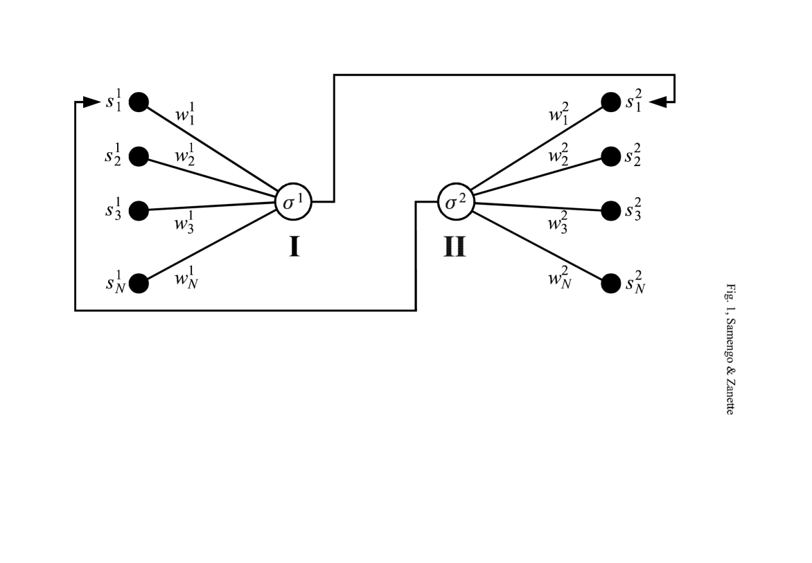
FIG. 1.: Two competing perceptrons.

We consider now two of these perceptrons (see Fig. 1), both with $N$ inputs. At each time step, the output of one of the perceptrons should be determined by the outputs of the other at the precedent steps. Indeed, this is the information available to each player on the strategy of the opponent. We associate therefore the inputs $s_{i}^{1}$ of perceptron I with the previous outputs $\sigma^{2}$ of perceptron II and vice versa, as

$$s_{i}^{1,2}(t)=\sigma^{2,1}(t-i),$$ (2)

$i=1,\dots,N$. Time steps are of unitary length.

Learning is a consequence of the comparison of the outputs of the two perceptrons at each time. If the outputs are identical perceptron II wins, and the synaptic weights $w_{i}^{1}$ of perceptron I are modified to produce a better prediction of the opponent’s output at the next round. Meanwhile, the synaptic weights $w_{i}^{2}$ of perceptron II can be left invariant, as they have led this perceptron to win the round. If, on the other hand, the outputs have been different, $w_{i}^{2}$ are modified and $w_{i}^{1}$ are maintained. A suitable algorithm for implementing this mechanism is the standard perceptron learning rule [2, 3, 13], which in our case implies

$$w_{i}^{1}(t+1)=w_{i}^{1}(t)-\eta\Theta[\sigma^{1}(t)\sigma^{2}(t)]s_{i}^{1}(t)\sigma^{2}(t)$$ (3)

and

$$w_{i}^{2}(t+1)=w_{i}^{2}(t)+\eta\Theta[-\sigma^{1}(t)\sigma^{2}(t)]\sigma^{1}(t)s_{i}^{2}(t),$$ (4)

with $i=1,\dots,N$ and $\eta=(1+N)^{-1}$. The Heaviside function $\Theta$ –where $\Theta(x)=1$ for $x\geq 0$ and $\Theta(x)=0$ for $x<0$– acts here as a mask, by selecting the perceptron whose synaptic weights are to be modified.

Suppose that the successive outputs of perceptron I are replaced by a periodic series of $\pm 1$ [14]. From the viewpoint of perceptron II, this is interpreted as the opponent’s choice of a trivial strategy. As a matter of fact, the perceptron convergence theorem [2, 11, 15] insures that if $N$ is large enough, i.e. if perceptron II’s memory is sufficiently long-ranged, the learning procedure stops and, from then on, perceptron II wins all rounds. When the period of the output series of perceptron I is lower than $N$, in fact, it can be straightforwardly shown that there is at least one set of synaptic weights $w^{2}_{i}$ that make perceptron II able to win at every round. The number of steps needed to compute these synaptic weights is of order $N^{3}$ [13], and can be tested numerically in our system. It is therefore not expected that when two large perceptrons are left to play freely one of them will adopt a short-period strategy.

III The system as a mapping: phase-space dynamics

Equations (1) to (4) define the dynamics of our system. They can be resumed in a $4N$-dimensional recursive mapping for the perceptron inputs and the synaptic weights only. The recursion equations are

$$\begin{array}[]{rl}s_{1}^{1,2}(t+1)=&S[\sum_{i}w_{i}^{2,1}(t)s_{i}^{2,1}(t)],\\ s_{i}^{1,2}(t+1)=&s_{i-1}^{1,2}(t)\ \ \ (i=2,\dots,N),\\ w_{i}^{1}(t+1)=&w_{i}^{1}(t)-\eta\Theta[s_{1}^{1}(t+1)s_{1}^{2}(t+1)]\\ &\times s_{1}^{1}(t+1)s_{i}^{1}(t)\ \ \ (i=1,\dots,N),\\ w_{i}^{2}(t+1)=&w_{i}^{2}(t)+\eta\Theta[-s_{1}^{1}(t+1)s_{1}^{2}(t+1)]\\ &\times s_{1}^{2}(t+1)s_{i}^{2}(t)\ \ \ (i=1,\dots,N).\end{array}$$ (5)

The phase space corresponding to this mapping is discrete. In fact, the inputs $s_{i}^{1,2}$ can adopt the two values $\pm 1$ only. Moreover, $w_{i}^{1,2}$ can have real values but they vary on a discrete set, since according to Eqs. (3) and (4) the variation of the synaptic weights has always the same modulus, $\left|\Delta w^{1,2}\right|=\eta$. Once the initial synaptic weights have been fixed, the discrete set of their possible future values is completely determined.

During the evolution, the synaptic weights can in principle run over an infinite set. However, though the synaptic weights are not expected to converge to fixed values but to continuously evolve as the game proceeds, it is reasonable to conjecture that they will not perform arbitrarily long excursions in phase space. To prove this conjecture, let us consider in detail the evolution of the synaptic weights, given by the two last equations in (5) or, equivalently, by Eqs. (3) and (4). These two equations can be written, respectively, as

$$\left\{\begin{array}[]{ll}w_{i}^{1}(t+1)=w_{i}^{1}(t)-\eta\sigma^{1}(t)s_{i}^{1}(t)&\mbox{if $\sigma^{1}(t)=\sigma^{2}(t)$}\\ w_{i}^{1}(t+1)=w_{i}^{1}(t)&\mbox{if $\sigma^{1}(t)=-\sigma^{2}(t)$},\\ \end{array}\right.$$ (6)

and

$$\left\{\begin{array}[]{ll}w_{i}^{2}(t+1)=w_{i}^{2}(t)-\eta\sigma^{2}(t)s_{i}^{2}(t)&\mbox{if $\sigma^{1}(t)=-\sigma^{2}(t)$}\\ w_{i}^{2}(t+1)=w_{i}^{2}(t)&\mbox{if $\sigma^{1}(t)=\sigma^{2}(t)$}.\\ \end{array}\right.$$ (7)

We now select one of the perceptrons and restrict the dynamics of its synaptic weights to the time steps where they are effectively modified, by simply ignoring the steps where no changes occur. The evolution equations can be written in vectorial form as

$${\bf w}(t+1)={\bf w}(t)-\eta S[{\bf w}(t)\cdot{\bf s}(t)]{\bf s}(t),$$ (8)

where the components of ${\bf w}$ and ${\bf s}$ are the synaptic weights and the inputs of the selected perceptron, respectively. We recall that $S(x)$ is the sign function. The scalar product ${\bf w}\cdot{\bf s}$ is defined in the usual way, cf. Eq. (1). Note that (8) holds for both perceptrons.

Let us now consider for a moment that, in Eq. (8), the vector ${\bf s}$ is independent of time. Under this assumption it is possible to reduce the system (8) to two equations for the quantities $p(t)={\bf s}\cdot{\bf w}(t)$ and $q(t)=|{\bf w}(t)|^{2}$, namely,

$$\begin{array}[]{ll}p(t+1)&=p(t)-(1-\eta)S[p(t)]\\ q(t+1)&=q(t)-2\eta|p(t)|+\eta(1-\eta).\end{array}$$ (9)

It can be easily seen from the first equation that $p(t)$ converges, after a certain transient, to a period-2 cycle. The two values of $p$ on this cycle, $p_{1}$ and $p_{2}$, satisfy the relation $p_{2}=p_{1}-1+\eta$. They depend on the initial conditions, but are always restricted to the intervals $0<p_{1}<1-\eta$ and $\eta-1<p_{2}<0$. Accordingly, $q(t)$ oscillates between two values, $q_{1}$ and $q_{2}$, defined by the initial conditions and related by $q_{2}=q_{1}-2\eta p_{1}+\eta(1-\eta)$. After the transient, the modulus of the vector ${\bf w}$ is therefore restricted to vary within the interval $[-W,W]$ with $W=\max\left\{\sqrt{q_{1}},\sqrt{q_{2}}\right\}$.

In summary, for fixed $\bf s$ the evolution given by Eq. (8) drives the synaptic weights towards a bounded domain whose size depends on the initial condition but which is always finite. We stress that this is valid for any choice of $\bf s$. Coming now back to the case of variable inputs, we note that the number of possible values for ${\bf s}(t)$ is also finite, and equals $2^{N}$. Equation (8) can therefore be thought of as the application, at each time step, of one of the $2^{N}$ transformations just studied. Since each of them contracts the space of synaptic weights towards a bounded region, after the transient ${\bf w}(t)$ will always evolve within the union of all those regions. Disregarding transient effects, the space of synaptic weights is then finite. Hence, the accessible phase space of mapping (5) is finite and discrete.

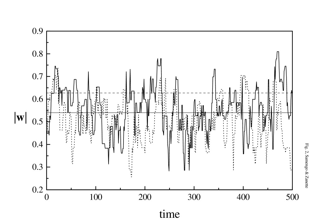
FIG. 2.: Module of the vector of synaptic weights for two competing perceptrons with $N=10$ inputs, as a function of time. Full and dotted curves correspond to $|{\bf w}^{1}|$ and $|{\bf w}^{2}|$, respectively. Full and dashed horizontal lines correspond to the analytical approximation for the average value of $|{\bf w}|$ for $N=10$ and $N\to\infty$, respectively.

As an illustration of the evolution of synaptic weights, we show in Fig. 2 the time dependence of $|{\bf w}|$ for both perceptrons. The initial weights were uniformly chosen at random in $(-0.2,0.2)$, and $N=10$. The horizontal lines in the plot stand for the theoretical values of the temporal average of $|{\bf w}|$ for $N=10$ (full line) and $N\to\infty$ (dashed line). These can be calculated by taking the square of Eq. (8), namely,

$$q(t+1)=q(t)-2\eta\sqrt{q(t)}|\widehat{\bf w}(t)\cdot{\bf s}(t)|+\eta(1-\eta)$$ (10)

with $\widehat{\bf w}={\bf w}/|{\bf w}|$. This recursion equation is analogous to the second of Eqs. (9). It can be seen that, for sufficiently large $N$, the average of $|\widehat{\bf w}(t)\cdot{\bf s}(t)|$ over time –or, equivalently, over random realizations of the vectors $\widehat{\bf w}$ and $\bf s$– becomes independent of $N$ and approaches the limit $\langle|\widehat{\bf w}\cdot{\bf s}|\rangle=\sqrt{2/\pi}\approx 0.798$. From Eq. (10), this implies that for large $N$:

$$\langle|{\bf w}|\rangle=\langle\sqrt{q}\rangle=\sqrt{\frac{\pi}{8}}\approx 0.627,$$ (11)

cf. [16]. A better approximation for finite $N$ is $\langle|{\bf w}|\rangle=\sqrt{\pi N(N-1)/8(N+1)^{2}}$. For $N=10$ this gives $\langle|{\bf w}|\rangle\approx 0.540$, which is the value plotted in Fig. 2. The average value of $|{\bf w}|$ provides an estimate for the size of the domain of phase space where the synaptic weights evolve after transients have elapsed. Note that the fact that $\langle|{\bf w}|\rangle$ approaches a constant for large $N$ implies that, in average, the synaptic weights are $w_{i}^{1,2}\sim 1/\sqrt{N}$.

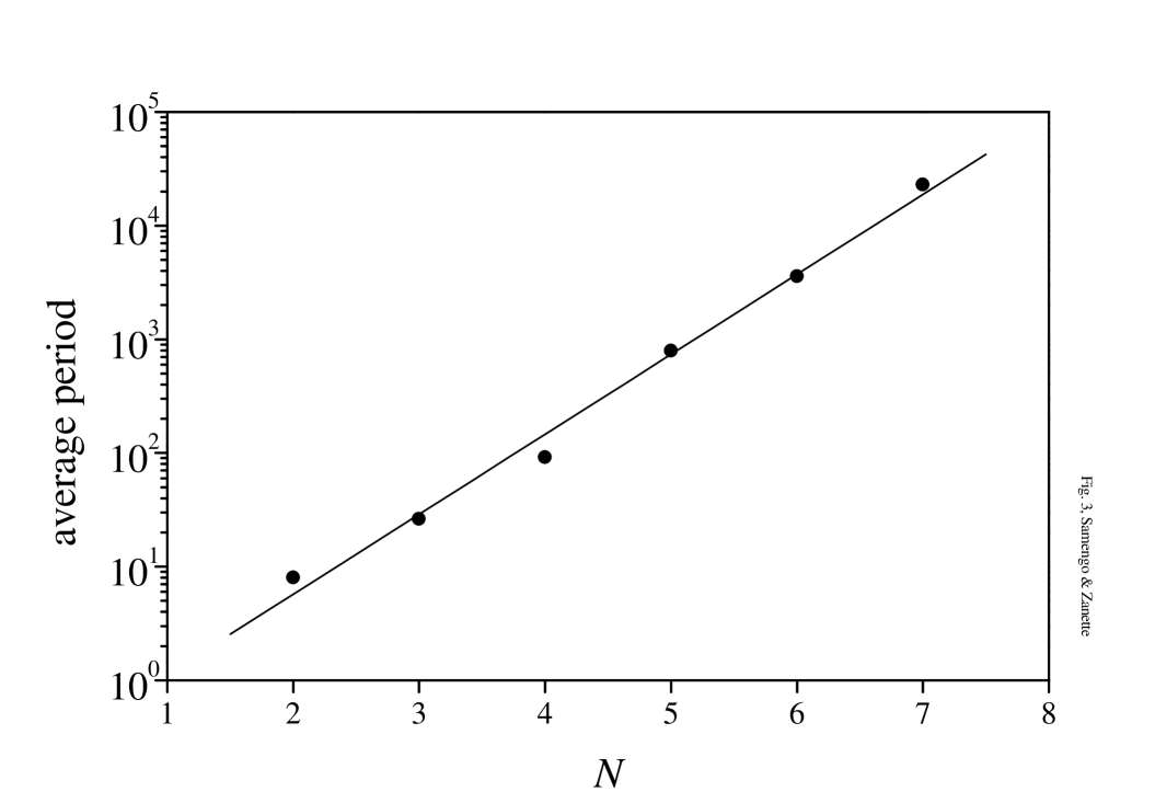
FIG. 3.: Average periods of the orbits of mapping (5), for different values of $N$. Notice the logarithmic scale in the vertical axis.

The main byproduct of the fact that for our system phase space is finite and discrete is that, after the transient has elapsed, the orbits will be periodic. It becomes therefore relevant to determine the length of the periods. In fact, if it resulted that orbits get typically trapped in short cycles, the problem would at once get uninteresting. We have measured the periods numerically, carrying out extensive series of $100$ to $1000$ realizations $6.4\times 10^{5}$ steps long, with $N$ ranging from $2$ to $10$. Initial conditions were chosen at random, with the synaptic weights uniformly distributed in $(-0.2,0.2)$. The system has always been found to reach a periodic orbit for $N<7$. For a fixed value of $N$, periods show typically a broad distribution. The average period has been found to increase exponentially with $N$, as shown in Fig. 3. For $N\geq 7$, not all the realizations displayed periodicity, indicating the occurrence of periods longer than our numerical realizations. Some test realizations for $N=10$ suggest that periods could grow beyond $10^{8}$ steps.

The system thus seems to have two well-differentiated time scales. On the one hand, there should be a time scale associated with learning, of order $N^{3}$. As stated above, in the case of a single perceptron being trained to predict a periodic series this is in fact the number of steps needed to compute all the synaptic weights. For the competing perceptrons, the length of the initial transient during which the system explores phase space to find the bounded region where it will evolve later, should be of the same order. On the other hand, we have a much longer “recursion” time scale, of order $A^{N}$ ($A\approx 5.05$, Fig. 3), associated with the periods of orbits inside that region. Though the two-perceptron dynamics is dissipative, it resembles in this aspect that of Hamiltonian systems with many degrees of freedom. Indeed, according to Poincaré’s theorem [17], Hamiltonian systems are recurrent and, at sufficiently long times, they visit an arbitrarily small neighborhood of their initial state. However, in a statistical description of their evolution, it is possible to identify much shorter time scales, related to the relaxation of fast variables [18].

At the level of recursion time scales, the dynamics of the two-perceptron system is in a sense trivial. Orbits are in fact periodic at long times, and the results of successive game rounds will be repeated ad infinitum. When, during a whole period, one of the perceptrons is able to gain even the smallest advantage over the other, this small difference will continuously accumulate producing, in the long run, an arbitrarily large bias in the result of the game. As in the case of large Hamiltonian systems, however, recursion times are far beyond the reach of our (numerical) experience as the size of the perceptrons increases. Therefore, most of the realizations of the two-perceptron game analyzed bellow will always be restricted to the transient period, previous to the appearance of periodicity. In this stage, the relevant time scale is the learning time, of order $N^{3}$. Within such times we expect the system to reach a kind of stationary playing regime where, if the learning algorithm is efficient, the outputs of the two perceptrons should imitate a random series of $\pm 1$. In the next section we study the statistical properties of these output series.

IV Statistical analysis of the game dynamics

Random properties in time series can be characterized in a variety of ways. In our case, where the relevant series are arrays of $\pm 1$, a suitable measure of time correlations is an information-like quantity [19]. As shown below, this quantity can be used to characterize the correlation between different series and, consequently, the correlation of a series with itself. It has the advantage of being additive, and is therefore appropriate when comparing numerical results. We thus begin by defining the mutual information of two time series.

Consider two dichotomic stochastic processes $S_{1}$ and $S_{2}$ that, at each time step, can adopt the values $\pm 1$ with certain probability distributions. Let $P(S_{1},S_{2})$ be the joint probability for the processes, and $P_{1}(S_{1})=\sum_{S_{2}}P(S_{1},S_{2})$ and $P_{2}(S_{2})=\sum_{S_{1}}P(S_{1},S_{2})$ their individual (marginal [20]) probabilities. A measure of the correlation between the two processes is given by the mutual information [19], defined as

$$I=\sum_{S_{1}=\pm 1}\sum_{S_{2}=\pm 1}P(S_{1},S_{2})\log_{2}\left[P(S_{1},S_{2})\over P_{1}(S_{1})P_{2}(S_{2})\right].$$ (12)

It can be shown that $I\geq 0$. For two uncorrelated processes, where $P(S_{1},S_{2})=P_{1}(S_{1})P_{2}(S_{2})$, the mutual information reaches its minimum, $I=0$. The maximal value of the mutual information is obtained for two identical stochastic processes, $S_{1}=S_{2}$, where $I=-P_{1}(+1)\log_{2}P_{1}(+1)-P_{1}(-1)\log_{2}P_{1}(-1)$. In particular, if $P_{1}(+1)=P_{1}(-1)=1/2$, we get $I=1$.

The definition of mutual information, Eq. (12), suggests immediately a way of introducing a measure of autocorrelation for a single dichotomic stochastic process $S$ at different times. In fact, associating $S_{1}(t)$ and $S_{2}(t)$ with $S(t)$ and $S(t+\tau)$, respectively, we can introduce the (two-time) autoinformation as

$$\begin{array}[]{rl}I(t,\tau)=\sum_{S(t)}\sum_{S(t+\tau)}&P[S(t),S(t+\tau)]\\ \\ &\times\log_{2}\left\{P[S(t),S(t+\tau)]\over P[S(t)]P[S(t+\tau)]\right\}.\end{array}$$ (13)

If $S$ is a stationary stochastic process [20] the autoinformation depends on the time interval $\tau$ only, $I\equiv I(\tau)$. If the successive values of $S$ are uncorrelated we have $I=0$, whereas for $\tau=0$ we get the maximal value $I(t,0)=-P(+1)\log_{2}P(+1)-P(-1)\log_{2}P(-1)$.

In practice, for a finite realization of the stochastic processes, the probabilities involved in Eqs. (12) and (13) are approximated by the corresponding frequencies, which can be computed by simple counting of the relevant occurrences. This approximation implies that in the case of uncorrelated processes the information can differ from zero, due to fluctuations in the finite sample under consideration. It can be shown that for a $T$-step realization of uncorrelated stochastic processes where the individual probabilities of the two possible values $\pm 1$ are equal, $P(+1)=P(-1)=1/2$, the probability distribution for the information to have a value $I$ is

$$p_{T}(I)=\sqrt{T\ln 2\over\pi I}\exp(-TI\ln 2),$$ (14)

for small $I$. The resulting mean value of the information is

$$\langle I\rangle=\int_{0}^{\infty}Ip_{T}(I)dI={1\over 2T\ln 2},$$ (15)

which decreases as $T^{-1}$ as the series size grows. For large $T$, $p_{T}(I)\to\delta(I)$, as expected. Thus, the distribution of values for the information computed from finite samples of size $T$ and its average are to be respectively compared with $p_{T}(I)$ and $\langle I\rangle$ in order to detect the presence of correlations.

We now consider two playing perceptrons with $N=10$, and apply the definition of autoinformation (13) to any of the two series of outputs, $S(t)\equiv\sigma^{1,2}(t)$. The outputs are recorded after the first $10^{4}$ steps have elapsed, in order to avoid nonstationary transient effects during the first stage of learning (of order $N^{3}$ [13]). The recorded series are $T=10^{4}$ steps long, and the results presented below correspond to averages over $5\times 10^{4}$ realizations.

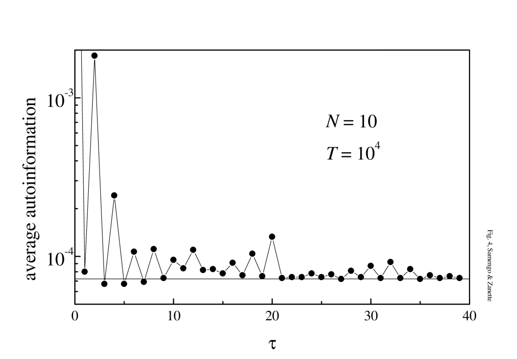
FIG. 4.: Average autoinformation for the output of one of the competing perceptrons as a function of the time interval $\tau$, measured in series of $10^{4}$ steps. Both perceptrons have $10$ inputs. The horizontal line corresponds to the average autoinformation expected for an uncorrelated series of the same length.

Figure 4 shows the measured average autoinformation as a function of $\tau$. The horizontal line corresponds to the average autoinformation (15) expected for an uncorrelated series with the present value of $T$, i.e. $\langle I\rangle\approx 7.2\times 10^{-5}$. We first note that, except for $\tau=2$ and $4$, the autoinformation of the output signal is always less that twice the value of $\langle I\rangle$ for a random series. This implies that each perceptron exhibits a quite good performance in generating a random sequence. There are however certain regular patterns that suggest the presence of small but nontrivial correlations. Indeed, the average autoinformation oscillates strongly for small $\tau$, reaching high levels for even values of $\tau$ and dropping abruptly for odd values of $\tau$. On average, these oscillations decrease as $\tau$ grows, but they reappear near $\tau=20$ and $30$. Realizations for other values of $N$ indicate that the oscillation amplitude decreases as $N$ grows, and that the “bursts” at which oscillations reappear occur when $\tau$ approaches integer multiples of $N$. The amplitude of these bursts decreases for larger multiples.

A more detailed description of the appearance of correlations in the output signals of the perceptrons is provided by the distribution of autoinformation values. Figure 5 displays the normalized frequencies of autoinformation values resulting from our sets of $5\times 10^{4}$ realizations of $10^{4}$-step series for various values of $\tau$. The curve corresponds to $p_{T}(I)$ for an uncorrelated series, Eq. (14). For $\tau=1$ practically no correlations are detected by the autoinformation. We note only a slight overpopulation for large $I$. On the other hand, for $\tau=2$, which corresponds to the largest deviation in the average autoinformation (see Fig. 4), the distribution is qualitatively different. It exhibits a maximum at a rather large value of the autoinformation ($I\approx 2\times 10^{-3}$) and, except for small values of $I$, it is systematically much larger than the distribution expected for a random series. At $\tau=10$, the distribution has a profile similar to that observed for $\tau=1$, but the overpopulation at the tail is noticeably larger. This overpopulation grows further during the bursts where oscillations reappear. The plot for $\tau=20$ shows the distribution at the first of these bursts. In contrast, for the intermediate values at which the average autoinformation plotted in Fig. 4 reaches the information of a random series, the corresponding distribution cannot be distinguished from $p_{T}(I)$.

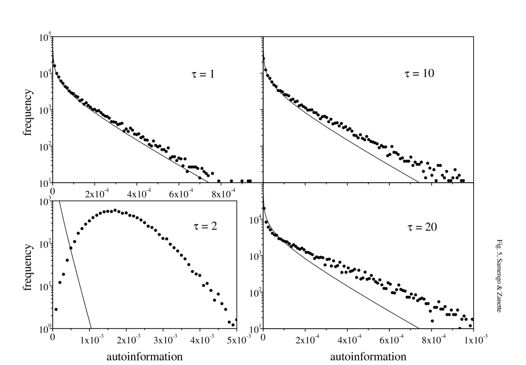
FIG. 5.: Normalized frequencies of autoinformation values obtained from $5\times 10^{4}$ series of $10^{4}$ steps, for several values of the time interval $\tau$. Both perceptrons have $10$ inputs. Curves correspond to the distribution expected for uncorrelated series of the same length, Eq. (14).

We have found that the oscillations of the average autoinformation shown in Fig. 4 are essentially a byproduct of the internal dynamics of each perceptron. In fact, if instead of using the opponent’s output, a perceptron is fed with a random series of $\pm 1$, the autoinformation of its own output oscillates as well. A detailed analysis of the output series reveals that, for even $\tau$, the product $\sigma(t)\sigma(t+\tau)$ is more frequently negative than positive. For instance, for $\tau=2$, the respective frequencies are about $0.52$ and $0.48$. We remark in passing that this small relative difference –of the order of a few percent– produces an increment larger than one order of magnitude in the autoinformation, which evidences the sensibility of this quantity as a measure of correlations. For larger values of $\tau$, the difference is even smaller. On the other hand, for odd $\tau$ no differences are detected.

In order to trace the origin of the correlations observed for even $\tau$, a careful analysis of the learning algorithm has to be carried out. We consider first the case of $\tau=2$. After two time steps, the vector of synaptic weights can be written as

$$\begin{array}[]{rl}{\bf w}(t+2)=&{\bf w}(t)-\eta\theta(t)\sigma(t){\bf s}(t)\\ &-\eta\theta(t+1)\sigma(t+1){\bf s}(t+1),\end{array}$$ (16)

where $\theta(t)=1$ if the weights have been modified at time $t$, and $\theta(t)=0$ otherwise [cf. Eq. (8)]. When the perceptron if fed with a random signal, $\theta(t)$ can be seen as a stochastic process with equal probabilities for its two values. The product of the outputs two steps apart is

$$\begin{array}[]{lll}\sigma(t)\sigma(t+2)&=&\sigma(t)S[{\bf w}(t+2)\cdot{\bf s}(t+2)]\\ &=&S[\sigma(t){\bf w}(t)\cdot{\bf s}(t+2)-\eta\theta(t){\bf s}(t)\cdot{\bf s}(t+2)\\ &&-\eta\theta(t+1)\sigma(t)\sigma(t+1){\bf s}(t+1)\cdot{\bf s}(t+2)]\end{array}$$ (17)

Numerical measurements of the right-hand side (r.h.s.) of this equation show that the first two terms in the argument of the sign function have zero mean and do not produce a net contribution to the sign of $\sigma(t)\sigma(t+2)$. The only contribution to the correlation is originated in the third term. To verify this fact analytically, we first note that

$$\begin{array}[]{l}{\bf w}(t+1)={\bf w}(t)[1+{\cal O}(1/\sqrt{N})],\\ {\bf s}(t+1)\cdot{\bf s}(t+2)={\bf s}(t)\cdot{\bf s}(t+1)[1+{\cal O}(1/\sqrt{N})].\end{array}$$ (18)

The first of these identities results from the fact that, as shown in the previous section, $w_{i}\sim 1/\sqrt{N}$ whereas, according to Eq. (5), its variation in one time step is given by $\eta\sim 1/N$. The second identity can be readily proven from the evolution of $s_{i}(t)$, also given in Eq. (5). Consequently, neglecting terms of order $1/\sqrt{N}$, the sign of the product $\sigma(t)\sigma(t+1){\bf s}(t+1)\cdot{\bf s}(t+2)$ can be approximated as follows:

$$\begin{array}[]{l}S[\sigma(t)\sigma(t+1){\bf s}(t+1)\cdot{\bf s}(t+2)]\\ \approx S\{[{\bf w}(t)\cdot{\bf s}(t)][{\bf w}(t)\cdot{\bf s}(t+1)][{\bf s}(t)\cdot{\bf s}(t+1)]\}.\end{array}$$ (19)

Note that the argument of the sign function in the r.h.s. of this equation is likely to be positive, since it is given by the product of the projections of two vectors, ${\bf s}(t)$ and ${\bf s}(t+1)$, along the direction of ${\bf w}(t)$ times their mutual scalar product. More explicitly,

$$\begin{array}[]{l}[{\bf w}(t)\cdot{\bf s}(t)][{\bf w}(t)\cdot{\bf s}(t+1)][{\bf s}(t)\cdot{\bf s}(t+1)]\\ =s_{w}^{2}(t)s_{w}^{2}(t+1)+s_{w}(t)s_{w}(t+1){\bf s}^{\prime}(t)\cdot{\bf s}^{\prime}(t+1),\end{array}$$ (20)

with $s_{w}={\bf w}\cdot{\bf s}$ and ${\bf s}^{\prime}={\bf s}-s_{w}\widehat{\bf w}$. The first term in the r.h.s. of this equation is always positive, whereas the second term is not expected to have a definite sign on average. Note moreover that the first term is of the order of unity, whereas the second term is of order $\sqrt{N}$. This implies that the relative importance of the positive contribution decreases as $N$ grows. Coming now back to Eq. (17) through Eq(19) it is clear that, when the synaptic weights are modified at time $t+1$ (i.e. $\theta(t+1)=1$), there is in average a negative contribution to $\sigma(t)\sigma(t+2)$, in agreement with numerical results. According to the above analysis, this correlation should become less important as $N$ grows. In fact, the autoinformation peak at $\tau=2$ is observed to decrease in the simulations.

For arbitrary $\tau$, the analysis can be repeated mutatis mutandis. We have

$$\begin{array}[]{rl}\sigma(t)\sigma(t+\tau)=S[&\sigma(t){\bf w}(t)\cdot{\bf s}(t+\tau)\\ &-\eta\sum_{t^{\prime}=0}^{\tau-1}\theta(t+t^{\prime})\sigma(t)\sigma(t+t^{\prime})\\ &\times{\bf s}(t+t^{\prime})\cdot{\bf s}(t+\tau)].\end{array}$$ (21)

Taking now into account that

$$\begin{array}[]{l}{\bf w}(t+t^{\prime})={\bf w}(t)[1+{\cal O}(\sqrt{t^{\prime}/N})],\\ {\bf s}(t+t^{\prime})\cdot{\bf s}(t+\tau)={\bf s}(t)\cdot{\bf s}(t+\tau-t^{\prime})[1+{\cal O}(\sqrt{t^{\prime}/N})],\end{array}$$ (22)

the sign of the product $\sigma(t)\sigma(t+t^{\prime}){\bf s}(t+t^{\prime})\cdot{\bf s}(t+\tau)$ in the sum of Eq. (21) can be approximately written as

$$\begin{array}[]{l}S[\sigma(t)\sigma(t+t^{\prime}){\bf s}(t+t^{\prime})\cdot{\bf s}(t+\tau)]\\ \approx S\{[{\bf w}(t)\cdot{\bf s}(t)][{\bf w}(t)\cdot{\bf s}(t+t^{\prime})][{\bf s}(t)\cdot{\bf s}(t+\tau-t^{\prime})]\}.\end{array}$$ (23)

The argument of the sign function in the r.h.s. of this equation has a positive contribution of the same type as in Eq. (19) when $t+t^{\prime}=t+\tau-t^{\prime}$, i.e. for $\tau=2t^{\prime}$. Therefore, in the realizations where $\theta(t+\tau/2)=1$ a negative contribution to $\sigma(t)\sigma(t+\tau)$ appears. This of course requires $\tau$ to be even. Since other contributions have no definite sign, peaks in the average autoinformation are expected for even values of $\tau$, as observed. Note moreover that the order $\sqrt{t^{\prime}/N}$ of the terms neglected in Eq. (23) increases with $t^{\prime}$, i.e. with $\tau$. This explains why the height of the peaks decreases as $\tau$ grows.

Along the same line of analysis, it is possible to explain the bursts where the autoinformation peaks reappear. Now, however, it is necessary to take into account both perceptrons. In fact, the output of a single perceptron fed with a random signal does not exhibit such bursts. They are rather a consequence of the interaction between the two perceptrons during the game. The analysis, whose details we omit here, shows that bursts are originated by a kind of bouncing effect in the transmission of information between the opponents. This bouncing effects is attenuated as $\tau$ grows, and decreases for larger perceptrons, as observed in the numerical simulations.

In summary, the statistical analysis of perceptron outputs at time scales larger than the learning stage but much shorter than the recursion times, reveals that the perceptrons are quite efficient players of the game of matching pennies. Even with a relatively small number of inputs, i.e. with a relatively short-ranged memory, their dynamics is able to generate quasi-random mixed strategies. We recall that this behavior originates spontaneously from the deterministic learning algorithm with which each player is endowed to outguess its opponent. Remaining correlations, which could in principle be exploited by a “smarter” opponent to obtain a net gain during the game, are overall small and can in fact be reduced systematically by increasing the memory range.

V Discussion

We have here considered an example of a fully deterministic learning system and explored its ability to behave stochastically. Concretely, we have coupled two deterministic perceptrons in such a way that they imitate two players of the game of matching pennies, trying to outguess each other. Since the optimal strategy for this game is a purely stochastic sequence of outputs, the learning process should lead the network dynamics to approach a random signal.

In the first place, we have observed that a perceptron producing a periodic signal can always be defeated by a sufficiently “smart” opponent, i.e. by a perceptron with a sufficiently large number of neurons. This kind of “dummy” player provides in fact a linearly separable set of examples for the learning of its opponent [2]. The learning task is thus to find a plane in the input space that separates the input states into two groups, namely those whose expected outputs are either $+1$ or $-1$. On the other hand, when the two competing perceptrons are allowed to learn the situation is pretty much different. Since both networks are looking for the best performance, they both change their strategies on line and, thus, they may well provide not only a nonlinearly separable set of examples, but also an inconsistent one. That is to say, at two different times any perceptron can give two different outputs from the same input state. This is the reason why the learning process does, in fact, not converge, and why the system is expected to spontaneously develop stochastic-like dynamics.

Our main conclusion is that, despite the fact that the overall dynamics is in the long run periodic, the perceptrons do learn to behave quasi-stochastically over moderately long time intervals. An information-theoretical statistical analysis of the output signals shows slight time correlations, to be ascribed to the deterministic coupling between the learning mechanism and the outputs themselves, which act as the inputs of the respective opponents. The effect of these correlations is observed to decrease gradually as the number of neurons in each perceptron grows. Two seemingly paradoxical aspects of this learning process deserve to be pointed out, because of their suggestive similarity with learning in humans (or other animals) entrained in a systematic activity such as a repetitive competition game. In the first place, the mutual search for regularity in the opponent’s behavior leads the whole system to develop highly irregular evolution over long times, which can hardly be distinguished from purely random dynamics. In the second place, we stress that competition can here be interpreted as a form of mutually supervised learning and, thus, results in a kind of collaboration between the opponents.

Some natural extensions of the present model are worth considering for future work. An important question to be addressed regards the case where the entangled perceptrons are not equal in size, i.e. they have different numbers of neurons. In such a situation, in fact, the above quoted correspondence of competition and collaboration could fail to hold. Preliminary results along this line (not presented in this paper) suggest however that the advantage of a larger perceptron is relatively small. Only very small networks ($N\sim 2$) are systematically defeated by larger opponents, as they typically fall in short-period cyclic orbits.

The perceptron-like structure of our networks is probably the simplest instance among a large class of possible architectures. Fully connected networks and multilayer structures have been shown to exhibit very high performance in learning tasks [2, 3, 19]. It would therefore be interesting to study how these more complex networks respond to mutually supervised learning. Finally, from the viewpoint of game theory, it would be relevant to analyze the dynamics of competing networks engaged in other games, especially, when ordinary optimization procedures do not lead to the optimal playing strategy. We mention, in particular, the iterated prisoner’s dilemma [21], which is attracting a great deal of attention as a paradigm of competition-collaboration interplay, and multiplayer minority games, recently studied by means of ensembles of globally coupled perceptrons [22]. Competing neural networks could contribute to a better understanding of the complex learning mechanisms involved in such kind of social interactions.

REFERENCES

- [1] W.A. Little, Math. Biosci. 19, 101 (1974).
- [2] J. Hertz, A. Krogh, and R. G. Palmer, Introduction to the Theory of Neural Computation (Addison Wesley, New york, 1991).
- [3] B. Müller, J. Reinhardt, and M.T. Strickland, Neural Networks (Springer, Berlin, 1995).
- [4] A.S. Mikhailov, Foundations of Synergetics I (Springer, Berlin, 1994) Chap. 6.
- [5] A.S. Lapedes and R.M. Farber, in Evolution, Learning and Cognition, edited by Y.S. Lee (World Scientific, Singapore, 1988) p. 331.
- [6] J.A. Anderson, Math. Biosci. 14, 197 (1972); J.J. Hopfield, Proc. Natl. Acad. Sci. USA 79, 2554 (1982).
- [7] Much work done by physicists on these lines has its roots and inspiration in some pioneer literature such as J. Maynard Smith, Evolution and the Theory of Games (Cambridge University Press, Cambridge, 1982).
- [8] G. Tesauro and T.J. Sejnowski, in Neural Information Processing Systems, edited by D.Z. Anderson (American Institute of Physics, New York, 1988) p. 794.
- [9] G. Owen, Game Theory (Academic Press, San Diego, 1995).
- [10] M. Gardner, Sci. Am. 217 (6), 127 (1967).
- [11] F. Rosenblatt, Principles of Neurodynamics (Spartan, New York, 1962).
- [12] B. Widrow and M.E. Hoff, Adaptive Switching Circuits, 1960 IRE WESCON Convention Record (IRE, New York, 1960); reprinted in Neurocomputing: Foundations of Research, edited by J.A. Anderson and E. Rosenfeld (MIT Press, Cambridge, 1988).
- [13] J.L. van Hemmen and R. Reimer, in Models of Neural Networks I, edited by E. Domany, J.L. van Hemmen, and K. Schulten (Springer, Berlin, 1995) Chap. 1.
- [14] M. Schröder, W. Kinzel, and I. Kanter, J. Phys. A 29, 7965 (1996).
- [15] M. Minsky ans S. Papert, Perceptrons: An Introduction to Computational Geometry (MIT Press, Cambridge, 1988).
- [16] H. Zhu and W. Kinzel, Neural Comput. 10, 2219 (1998).
- [17] V.I. Arnold, Mathematical Methods of Classical Mechanics (Springer, Berlin, 1989).
- [18] N.G. van Kampen, Phys. Rep. 124, 69 (1985).
- [19] E.T. Rolls and A. Treves, Neural Networks and Brain Function (Oxford University Press, Oxford, 1998).
- [20] N.G. van Kampen, Stochastic Processes in Physics and Chemistry (North-Holland, Amsterdam, 1992).
- [21] R. Axelrod, The Evolution of Cooperation (Basic Books, New York, 1984).
- [22] W. Kinzel, R. Metzler, and I. Kanter, cond-mat/9906058.