Computer simulation of uniformly heated granular fluids

Abstract

Direct Monte Carlo simulations of the Enskog-Boltzmann equation for a spatially uniform system of smooth inelastic spheres are performed. In order to reach a steady state, the particles are assumed to be under the action of an external driving force which does work to compensate for the collisional loss of energy. Three different types of external driving are considered: (a) a stochastic force, (b) a deterministic force proportional to the particle velocity and (c) a deterministic force parallel to the particle velocity but constant in magnitude. The Enskog-Boltzmann equation in case (b) is fully equivalent to that of the homogeneous cooling state (where the thermal velocity monotonically decreases with time) when expressed in terms of the particle velocity relative to the thermal velocity. Comparison of the simulation results for the fourth cumulant and the high energy tail with theoretical predictions derived in cases (a) and (b) [T. P. C. van Noije and M. H. Ernst, Gran. Matt. 1, 57 (1998)] shows a good agreement. In contrast to these two cases, the deviation from the Maxwell-Boltzmann distribution is not well represented by Sonine polynomials in case (c), even for low dissipation. In addition, the high energy tail exhibits an underpopulation effect in this case.

1 Introduction

Most of the recent studies of rapid granular flow C90 are based on the Enskog equation for the velocity distribution function $f(\mathbf{r},\mathbf{v},t)$ of an assembly of inelastic hard spheres BDS97 . In the special case of a spatially uniform state, the Enskog equation reads

$$\frac{\partial}{\partial t}f(\mathbf{v}_{1},t)+\mathcal{F}f(\mathbf{v}_{1},t)=\chi I[\mathbf{v}_{1}|f(t),f(t)],$$ (1)

where

$$I[\mathbf{v}_{1}|f(t),f(t)] \equiv \sigma^{d-1}\int d\mathbf{v}_{2}\int d\widehat{\boldsymbol{\sigma}}\,\Theta(\mathbf{v}_{12}\cdot\widehat{\boldsymbol{\sigma}})(\mathbf{v}_{12}\cdot\widehat{\boldsymbol{\sigma}})$$

$$\times\left[\alpha^{-2}f(\mathbf{v}_{1}^{\prime\prime},t)f(\mathbf{v}_{2}^{\prime\prime},t)-f(\mathbf{v}_{1},t)f(\mathbf{v}_{2},t)\right].$$

In Eq. (1) $\mathcal{F}$ is an operator representing the effect of an external force (if it exists), $\chi$ is the pair correlation function at contact and $I$ is the collision operator. In Eq. (1), $d$ is the dimensionality of the system, $\sigma$ is the diameter of the spheres, $\mathbf{v}_{12}\equiv\mathbf{v}_{1}-\mathbf{v}_{2}$ is the relative velocity of the colliding particles, $\widehat{\boldsymbol{\sigma}}$ is a unit vector directed along the line of centers from the sphere $1$ to the sphere $2$, $\Theta$ is the Heaviside step function and $\alpha<1$ is the coefficient of normal restitution, here assumed to be constant. In addition, $(\mathbf{v}_{1}^{\prime\prime},\mathbf{v}_{2}^{\prime\prime})$ are the precollisional velocities yielding $(\mathbf{v}_{1},\mathbf{v}_{2})$ as the postcollisional ones, i.e. $\mathbf{v}_{1,2}^{\prime\prime}=\mathbf{v}_{1,2}\mp\frac{1}{2}(1+\alpha^{-1})(\mathbf{v}_{12}\cdot\widehat{\boldsymbol{\sigma}})\widehat{\boldsymbol{\sigma}}$. Except for the presence of the factor $\chi$, which accounts for the increase of the collision frequency due to excluded volume effects, the Enskog equation for uniform states, Eq. (1), becomes identical with the Boltzmann equation.

In the case of elastic particles ($\alpha=1$) and in the absence of external forcing ($\mathcal{F}=0$), it is well known that the long-time solution of Eq. (1) is the Maxwell-Boltzmann equilibrium distribution function, $f(\mathbf{v},t)\to nv_{0}^{-d}\phi(\mathbf{v}/v_{0})$, $\phi(\mathbf{c})\equiv\pi^{-d/2}e^{-c^{2}}$, where $n$ is the number density, $v_{0}=(2\langle v^{2}\rangle/d)^{1/2}$ is the thermal velocity and $\mathbf{c}=\mathbf{v}/v_{0}$ is the reduced velocity. On the other hand, if the particles are inelastic ($\alpha<1$) and $\mathcal{F}=0$, a steady state is not possible in uniform situations since, due to the dissipation of energy through collisions, the thermal velocity $v_{0}(t)$ decreases monotonically with time. Regardless of the initial uniform state, the solution of Eq. (1) tends to the so-called homogeneous cooling state GS95 ; NE96 ; NE98 ; BMC96 , characterized by the fact that the time dependence occurs only through the thermal velocity $v_{0}(t)$: $f(\mathbf{v},t)\to nv_{0}^{-d}(t)\widetilde{f}(\mathbf{v}/v_{0}(t))$. In addition, $\widetilde{f}(\mathbf{c})$ deviates from a Maxwellian, $\widetilde{f}(\mathbf{c})\neq\phi(\mathbf{c})$, as measured by the fourth cumulant

$$a_{2}\equiv\frac{d}{d+2}\frac{\langle v^{4}\rangle}{\langle v^{2}\rangle^{2}}-1=\frac{4}{d(d+2)}\langle c^{4}\rangle-1,$$ (3)

where

$$\langle c^{p}\rangle\equiv\int d\mathbf{c}\,c^{p}\widetilde{f}(\mathbf{c}).$$ (4)

By expanding $\widetilde{f}(\mathbf{c})/\phi(\mathbf{c})$ in a set of Sonine polynomials $\{S_{p}(c^{2})\}$ and neglecting the terms beyond $p=2$, van Noije and Ernst NE96 ; NE98 have estimated the value of $a_{2}$:

$$a_{2}(\alpha)\simeq\frac{16(1-\alpha)(1-2\alpha^{2})}{9+24d-\alpha(41-8d)+30(1-\alpha)\alpha^{2}}.$$ (5)

The above expression corrects an algebraic error in a previous calculation of $a_{2}$ in the three-dimensional case GS95 . According to Eq. (5), $a_{2}$ changes sign at $\alpha=1/\sqrt{2}\simeq 0.71$. By using the same method, Garzó and Dufty GD99 have recently extended the evaluation of $a_{2}$ to a binary mixture of hard spheres. The accuracy of Eq. (5) has been quantitatively confirmed by Brey et al. BMC96 from Monte Carlo simulations of the Boltzmann equation for hard spheres ($d=3$) in the range $0.7\leq\alpha\leq 1$. As a complementary measure of the departure of $\widetilde{f}(\mathbf{c})$ from $\phi(\mathbf{c})$, Esipov and Pöschel EP97 and van Noije and Ernst NE98 have analyzed the high energy tail of the distribution function and have found an asymptotic behavior of the form

$$\log\widetilde{f}(\mathbf{c})\sim-c,$$ (6)

in contrast to $\log\phi(\mathbf{c})\sim-c^{2}$. The high energy tail (6) has been confirmed by simulations in the case of hard disks ($d=2$) BCR99 .

In order to reach a steady state, energy injection is needed to compensate for the energy dissipated through collisions. This can be achieved by vibration of vessels ER89 or in fluidized beds IH95 . The same effect can be obtained by means of external driving forces acting locally on each particle WM96 . Borrowing a terminology frequently used in nonequilibrium molecular dynamics of elastic particles EM90 , we will call this type of external forces “thermostats”. In general, the equation of motion for a particle $i$ is then

$$m\dot{\mathbf{v}}_{i}=\mathbf{F}_{i}^{\mbox{\scriptsize coll}}+\mathbf{F}_{i}^{\mbox{\scriptsize th}},$$ (7)

where $m$ is the mass of a particle, $\mathbf{F}_{i}^{\mbox{\scriptsize coll}}$ is the force due to collisions and $\mathbf{F}_{i}^{\mbox{\scriptsize th}}$ is the thermostat force. Williams and MacKintosh WM96 introduced a stochastic force assumed to have the form of a Gaussian white noise:

$$\langle\mathbf{F}_{i}^{\mbox{\scriptsize th}}(t)\rangle=\mathbf{0},\quad\langle\mathbf{F}_{i}^{\mbox{\scriptsize th}}(t)\mathbf{F}_{j}^{\mbox{\scriptsize th}}(t^{\prime})\rangle=\mathsf{I}m^{2}\xi_{0}^{2}\delta_{ij}\delta(t-t^{\prime}),$$ (8)

where $\mathsf{I}$ is the $d\times d$ unit matrix and $\xi_{0}^{2}$ represents the strength of the correlation. The corresponding operator $\mathcal{F}$ appearing in Eq. (1) has a Fokker-Planck form NE98 :

$$\mathcal{F}f(\mathbf{v}_{1})=-\frac{\xi_{0}^{2}}{2}\left(\frac{\partial}{\partial\mathbf{v}_{1}}\right)^{2}f(\mathbf{v}_{1}).$$ (9)

Van Noije and Ernst NE98 have studied the stationary solution of the uniform equation (1) with the thermostat (9). They have found for the coefficient $a_{2}$ defined by Eq. (3) the value

$$a_{2}(\alpha)\simeq\frac{16(1-\alpha)(1-2\alpha^{2})}{73+56d-3\alpha(35+8d)+30(1-\alpha)\alpha^{2}}.$$ (10)

The high energy tail is NE98

$$\log\widetilde{f}(\mathbf{c})\sim-c^{3/2}.$$ (11)

Of course, deterministic thermostats can also be used. For instance, the use of Gauss’s principle of least constraint leads to the thermostat force EM90

$$\mathbf{F}_{i}^{\mbox{\scriptsize th}}=m\zeta\mathbf{v}_{i},$$ (12)

where $\zeta$ is a positive constant. In this case,

$$\mathcal{F}f(\mathbf{v}_{1})=\zeta\frac{\partial}{\partial\mathbf{v}_{1}}\cdot\left[\mathbf{v}_{1}f(\mathbf{v}_{1})\right].$$ (13)

It is interesting pointing out that the Enskog-Boltzmann equation (1) for the above Gaussian thermostat force is formally identical with the equation for the homogeneous cooling state (i.e. with $\mathcal{F}=0$) when both equations are expressed in terms of the reduced distribution $\widetilde{f}(\mathbf{c})$ (see Sect. 2). As a consequence, the results (5) and (6) apply to this thermostatted case as well.

The differences between Eqs. (5) and (10) and between (6) and (11) illustrate the influence of the thermostat force on the departure of the steady-state distribution function from the Maxwell-Boltzmann distribution. In the case of the stochastic force, Eq. (9), $\widetilde{f}(\mathbf{c})$ is closer to $\phi(\mathbf{c})$ than in the case of the Gaussian force, Eq. (13), since in the former case $a_{2}$ and the high energy overpopulation are smaller than in the latter case. Of course, other types of thermostats are also possible. For example, a different choice for a deterministic thermostat is

$$\mathbf{F}_{i}^{\mbox{\scriptsize th}}=mg\widehat{\mathbf{v}}_{i},$$ (14)

where $\widehat{\mathbf{v}}_{i}\equiv{\mathbf{v}}_{i}/v_{i}$. While the Gaussian force, Eq. (12), is proportional to the velocity of the particle, Eq. (14) corresponds to a force that is parallel to the direction of motion but constant in magnitude. The corresponding operator $\mathcal{F}$ is

$$\mathcal{F}f(\mathbf{v}_{1})=\frac{g}{v_{1}}\left\{\frac{\partial}{\partial\mathbf{v}_{1}}\cdot\left[\mathbf{v}_{1}f(\mathbf{v}_{1})\right]-f(\mathbf{v}_{1})\right\}.$$ (15)

The aim of this paper is to present direct Monte Carlo simulations of Eq. (1) with the three choices for the thermostat, Eqs. (9), (13) and (15). In the cases of the stochastic and the Gaussian thermostats, we will confirm the tails (11) and (6) and will check the accuracy of the estimates (10) and (5). In the latter case, however, we will see that a better agreement with simulation results for $\alpha<0.5$ is obtained if an estimate slightly different from (5) is used. The simulation results corresponding to the non-Gaussian thermostat (15) show that, in contrast to what happens in the two previous cases, $a_{2}$ remains negative for all $\alpha$. This feature is qualitatively captured by an estimate derived from a Sonine approximation. In this problem, however, the Sonine polynomials do not constitute a good set for the expansion of $\widetilde{f}(\mathbf{c})/\phi(\mathbf{c})$ and, consequently, the estimate is not quantitatively good. Besides, the high energy tail is of the form $\log\widetilde{f}(\mathbf{c})\sim-c^{2}$, but with a coefficient different from that of the Maxwell-Boltzmann distribution.

The organization of this paper is as follows. The theoretical analysis is reviewed in Sect. 2. The computer simulation method employed to solve numerically the uniform Enskog-Boltzmann equation is described in Sect. 3. The results are presented and compared with the theoretical predictions in Sect. 4. The paper ends with a summary and discussion in Sect. 5.

2 Theoretical predictions

In the steady state, the Enskog-Boltzmann equation (1) can be expressed in terms of the reduced velocity distribution function $\widetilde{f}(\mathbf{c})$ as

$$\widetilde{\mathcal{F}}\widetilde{f}(\mathbf{c}_{1})=\chi\widetilde{I}[\mathbf{c}_{1}|\widetilde{f},\widetilde{f}],$$ (16)

where

$$\widetilde{I}[\mathbf{c}_{1}|\widetilde{f},\widetilde{f}] \equiv \int d\mathbf{c}_{2}\int d\widehat{\boldsymbol{\sigma}}\,\Theta(\mathbf{c}_{12}\cdot\widehat{\boldsymbol{\sigma}})(\mathbf{c}_{12}\cdot\widehat{\boldsymbol{\sigma}})$$ (17)

$$\times\left[\alpha^{-2}\widetilde{f}(\mathbf{c}_{1}^{\prime\prime})\widetilde{f}(\mathbf{c}_{2}^{\prime\prime})-\widetilde{f}(\mathbf{c}_{1})\widetilde{f}(\mathbf{c}_{2})\right].$$

The reduced operator $\widetilde{\mathcal{F}}$ for the stochastic [Eq. (9)], Gaussian [Eq. (13)] and non-Gaussian [Eq. (15)] thermostats, is

$$\widetilde{\mathcal{F}}\widetilde{f}(\mathbf{c}_{1})=-\frac{\xi_{0}^{2}}{2v_{0}^{3}n\sigma^{d-1}}c_{1}^{-(d-1)}\frac{\partial}{\partial{c}_{1}}\left[c_{1}^{d-1}\frac{\partial\widetilde{f}(\mathbf{c}_{1})}{\partial c_{1}}\right],$$ (18)

$$\widetilde{\mathcal{F}}\widetilde{f}(\mathbf{c}_{1})=\frac{\zeta}{v_{0}n\sigma^{d-1}}c_{1}^{-(d-1)}\frac{\partial}{\partial{c}_{1}}\left[c_{1}^{d}\widetilde{f}(\mathbf{c}_{1})\right],$$ (19)

$$\widetilde{\mathcal{F}}\widetilde{f}(\mathbf{c}_{1})=\frac{g}{v_{0}^{2}n\sigma^{d-1}}c_{1}^{-(d-1)}\frac{\partial}{\partial{c}_{1}}\left[c_{1}^{d-1}\widetilde{f}(\mathbf{c}_{1})\right],$$ (20)

respectively. In Eqs. (18)–(20) we have already taken into account that the distribution function must be isotropic in the steady state. Equation (16) with the term (19) is fully equivalent to Eq. (10) of Ref. NE98 , the latter being derived in the context of the homogeneous cooling state. This formal equivalence between the free evolving state and the one controlled by a Gaussian external force is also present in the case of elastic particles interacting via arbitrary power-law potentials in homogeneous situations GSB90 or via the Maxwell potential in the uniform shear flow DSBR86 .

2.1 Stochastic thermostat

For the sake of completeness, we summarize now some of the results obtained in Ref. NE98 . In order to characterize the deviation of $\widetilde{f}(\mathbf{c})$ from $\phi(\mathbf{c})$ by means of the cumulant (3), it is useful to consider the hierarchy of moment equations. Multiplying both sides of Eq. (16) by $c_{1}^{p}$ and integrating over $\mathbf{c}_{1}$, we get

$${\mu_{p}}={\mu_{2}}\frac{p(p+d-2)}{2d}\langle c^{p-2}\rangle$$ (21)

for the stochastic thermostat, where we have defined

$$\mu_{p}\equiv-\int d\mathbf{c}\,c^{p}\widetilde{I}[\mathbf{c}|\widetilde{f},\widetilde{f}].$$ (22)

In Eq. (21) we have taken into account the normalization condition $\langle c^{0}\rangle=1$, so that $\mu_{2}=d{\xi_{0}^{2}}/{v_{0}^{3}\chi n\sigma^{d-1}}$. In the special case of $p=4$, Eq. (21) becomes

$${\mu_{4}}=(d+2){\mu_{2}},$$ (23)

where we have used the fact that, by definition, $\langle c^{2}\rangle=d/2$. Equations (22) and (23) are still exact. To get an approximate expression for $a_{2}(\alpha)$, three steps will be taken NE98 . First, we assume that $\widetilde{f}$ can be well described by the simplest Sonine approximation, at least for the velocities relevant to the evaluation of $a_{2}$. Thus,

$$\widetilde{f}(\mathbf{c})\simeq\phi(\mathbf{c})\left[1+a_{2}S_{2}(c^{2})\right],$$ (24)

where

$$S_{2}(x)=\frac{1}{2}x^{2}-\frac{d+2}{2}x+\frac{d(d+2)}{8}.$$ (25)

The approximation (24) is justified by the fact that $a_{2}$ is expected to be small. The second step consists of inserting Eq. (24) into Eq. (22) and neglecting terms nonlinear in $a_{2}$. For $\mu_{2}$ and $\mu_{4}$ the results are NE98

$$\mu_{p}\simeq\mu_{p}^{(0)}+\mu_{p}^{(1)}a_{2},$$ (26)

with

$$\mu_{2}^{(0)}\equiv\frac{\pi^{(d-1)/2}}{\sqrt{2}\Gamma(d/2)}(1-\alpha^{2}),$$ (27)

$$\mu_{2}^{(1)}\equiv\frac{3}{16}\mu_{2}^{(0)},$$ (28)

$$\mu_{4}^{(0)}\equiv\left(d+\frac{3}{2}+\alpha^{2}\right)\mu_{2}^{(0)},$$ (29)

$$\mu_{4}^{(1)}\equiv\left[\frac{3}{32}\left(10d+39+10\alpha^{2}\right)+\frac{d-1}{1-\alpha}\right]\mu_{2}^{(0)}.$$ (30)

In the third step, the approximations (26) with $p=2\mbox{ and }4$ are inserted into the exact equation (23) and $a_{2}$ is obtained from the resulting linear equation:

$$a_{2}\simeq-\frac{\mu_{4}^{(0)}-(d+2)\mu_{2}^{(0)}}{\mu_{4}^{(1)}-(d+2)\mu_{2}^{(1)}}.$$ (31)

This is the result derived by van Noije and Ernst NE98 , Eq. (10). It must be pointed out that a certain degree of ambiguity is present in this last step. For instance, if Eq. (23) were written as $\mu_{4}/\mu_{2}=d+2$, we could expand the ratio $\mu_{4}/\mu_{2}$ in powers of $a_{2}$ and neglect nonlinear terms to find

$$a_{2} \simeq -\frac{\mu_{4}^{(0)}-(d+2)\mu_{2}^{(0)}}{\mu_{4}^{(1)}-\mu_{2}^{(1)}\mu_{4}^{(0)}/\mu_{2}^{(0)}}$$ (32)

$$= \frac{4(1-\alpha)(1-2\alpha^{2})}{19+14d-3\alpha(9+2d)+6(1-\alpha)\alpha^{2}}.$$

However, since $a_{2}$ is indeed small ($|a_{2}|<0.1$), Eqs. (10) and (32) give practically identical results, the maximum deviation being less than about 0.001.

Now we consider the high energy tail. In general, the collision integral can be decomposed into a gain and a loss term: $\widetilde{I}[\mathbf{c}_{1}|\widetilde{f},\widetilde{f}]=\widetilde{I}_{g}[\mathbf{c}_{1}|\widetilde{f},\widetilde{f}]-\widetilde{I}_{l}[\mathbf{c}_{1}|\widetilde{f},\widetilde{f}]$. For large $c_{1}$ the loss term can be approximated as

$$\widetilde{I}_{l}[\mathbf{c}_{1}|\widetilde{f},\widetilde{f}] = \beta_{1}\int d\mathbf{c}_{2}\,c_{12}\widetilde{f}(\mathbf{c}_{1})\widetilde{f}(\mathbf{c}_{2})$$ (33)

$$\approx \beta_{1}c_{1}\widetilde{f}(\mathbf{c}_{1}),$$

where $\beta_{1}$ is defined by Eq. (84). Let us assume that for large velocities the gain term is negligible versus the loss term, i.e.

$$\lim_{c_{1}\to\infty}\frac{\widetilde{I}_{g}[\mathbf{c}_{1}|\widetilde{f},\widetilde{f}]}{\widetilde{I}_{l}[\mathbf{c}_{1}|\widetilde{f},\widetilde{f}]}=0.$$ (34)

In that case, the Enskog-Boltzmann equation for the stochastic thermostat becomes

$$\frac{\mu_{2}}{2d}c^{-(d-1)}\frac{\partial}{\partial{c}}\left[c^{d-1}\frac{\partial\widetilde{f}(\mathbf{c})}{\partial c}\right]\approx\beta_{1}c\widetilde{f}(\mathbf{c}).$$ (35)

The solution of this equation for large $c$ is

$$\widetilde{f}(\mathbf{c})\approx K\exp\left(-Ac^{3/2}\right),\quad A\equiv\frac{2}{3}\left(\frac{2d\beta_{1}}{\mu_{2}}\right)^{1/2},$$ (36)

where $K$ is an undetermined constant. By arguments given in Ref. NE98 , it can be seen that the result (36) is indeed consistent with the assumption (34). Equation (36) shows an overpopulation with respect to the Maxwell-Boltzmann tail. On the other hand, as $\alpha\to 1$, the amplitude $A$ diverges as $(1-\alpha)^{-1/2}$, thus indicating that the overpopulation effect is restricted to larger and larger energies in the limit $\alpha\to 1$.

2.2 Gaussian thermostat

In the case of the deterministic Gaussian thermostat, Eq. (19), the moment equation is

$$\mu_{p}=\mu_{2}\frac{p}{d}\langle c^{p}\rangle,$$ (37)

where now $\mu_{2}=d{\zeta}/{v_{0}\chi n\sigma^{d-1}}$. If we set $p=4$,

$$\mu_{4}=(d+2)(1+a_{2})\mu_{2},$$ (38)

where we have made use of Eq. (3). Substituting the approximation (26) and neglecting terms nonlinear in $a_{2}$, we get

$$a_{2}\simeq-\frac{\mu_{4}^{(0)}-(d+2)\mu_{2}^{(0)}}{\mu_{4}^{(1)}-(d+2)(\mu_{2}^{(1)}+\mu_{2}^{(0)})},$$ (39)

which is the same as Eq. (5). There exists again some arbitrariness about the use of the exact equation (38) in connection with the approximation (26). If we rewrite (38) as $\mu_{4}/\mu_{2}=(d+2)(1+a_{2})$ and neglect nonlinear terms, the resulting $a_{2}$ is fairly close to Eq. (39). On the other hand, if we start from $\mu_{4}/(1+a_{2})=(d+2)\mu_{2}$, the result is

$$a_{2} \simeq -\frac{\mu_{4}^{(0)}-(d+2)\mu_{2}^{(0)}}{\mu_{4}^{(1)}-\mu_{4}^{(0)}-(d+2)\mu_{2}^{(1)}}$$ (40)

$$= \frac{16(1-\alpha)(1-2\alpha^{2})}{25+24d-\alpha(57-8d)-2(1-\alpha)\alpha^{2}}.$$

The estimates (5) and (40) practically coincide in the region $0.5<\alpha\leq 1$. However, they visibly separate for larger dissipation. In the interval $0<\alpha<0.3$, the values given by Eq. (5) are 12%–20% ($d=3$) or 18%–28% ($d=2$) larger than those given by Eq. (40). As we will see later, the simulation results indicate that Eq. (40) is a better estimate than Eq. (5).

For large $c$ the Enskog-Boltzmann equation becomes

$$\frac{\mu_{2}}{d}c^{-(d-1)}\frac{\partial}{\partial{c}}\left[c^{d}\widetilde{f}(\mathbf{c})\right]\approx-\beta_{1}c\widetilde{f}(\mathbf{c}),$$ (41)

where we have used Eqs. (33) and (34). Its solution is

$$\widetilde{f}(\mathbf{c})\approx K\exp\left(-Ac\right),\quad A\equiv\frac{d\beta_{1}}{\mu_{2}}.$$ (42)

Again, this result is seen to be consistent with (34) NE98 . Equation (42) indicates an overpopulation effect even larger than with the stochastic thermostat.

2.3 Non-Gaussian thermostat

Now we consider the deterministic non-Gaussian thermostat (14), represented by the operator (20). To the best of our knowledge, this external force has not been analyzed before. The corresponding moment equation is

$$\mu_{p}=\mu_{2}\frac{p}{2}\frac{\langle c^{p-1}\rangle}{\langle c\rangle},$$ (43)

where $\mu_{2}={2g}{\langle c\rangle}/{v_{0}^{2}\chi n\sigma^{d-1}}$. In particular,

$$\mu_{4}=2\mu_{2}\frac{\langle c^{3}\rangle}{\langle c\rangle}.$$ (44)

In contrast to the two previous cases, now the even collisional moments $\mu_{p}$ are coupled to the odd moments $\langle c^{p-1}\rangle$, and vice versa. In terms of the energy variable $\epsilon=c^{2}$, this means that the integer collisional moments are coupled to the half-integers energy moments. This is related to the fact that the force (14) is singular at $\epsilon=0$. As a consequence, while $\widetilde{f}(\mathbf{c})$ is expected to be close to the Maxwellian $\phi(\mathbf{c})$, the ratio $\widetilde{f}(\mathbf{c})/\phi(\mathbf{c})$ is singular at $\epsilon=0$ and thus it is not well represented by an expansion in $\{S_{p}(\epsilon)\}$. To be more precise, let us define the function $\Delta(c)$ by the equation

$$\widetilde{f}(\mathbf{c})=\phi(\mathbf{c})\left[1+a_{2}\Delta(c)\right].$$ (45)

Therefore,

$$\int d\mathbf{c}\,\phi(\mathbf{c})\Delta(c)=\int d\mathbf{c}\,\phi(\mathbf{c})c^{2}\Delta(c)=0,$$ (46)

$$\int d\mathbf{c}\,\phi(\mathbf{c})c^{4}\Delta(c)=\frac{d(d+2)}{4}.$$ (47)

The polynomial $S_{2}(c^{2})$ verifies the above equalities. As a matter of fact, $\Delta(c)\simeq S_{2}(c^{2})$ in the cases of the thermostats (18) and (19). This is not so, however, in the case of (20), even in the limit of low dissipation. As we will see in Sect. 4, $\left.\partial\Delta(c)/\partial c\right|_{c=0}\neq 0$, what indicates that $\Delta(c)$ is essentially different from a polynomial in $c^{2}$. All of this complicates the evaluation of $a_{2}$. Nevertheless, since $\Delta(c)$ and $S_{2}(c^{2})$ share the moments of degrees 0, 2 and 4 [cf. Eqs. (46) and (47)], we can expect to obtain a crude estimate of $a_{2}$ by assuming that in the calculation of $\langle c\rangle$, $\langle c^{3}\rangle$, $\mu_{2}$ and $\mu_{4}$ we can replace $\Delta(c)$ by $S_{2}(c^{2})$. If that were the case, $\mu_{2}$ and $\mu_{4}$ would be given by Eqs. (26)–(30) and

$$\langle c\rangle\simeq\frac{\Gamma((d+1)/2)}{\Gamma(d/2)}\left(1-\frac{1}{8}a_{2}\right),$$ (48)

$$\langle c^{3}\rangle\simeq\frac{\Gamma((d+3)/2)}{\Gamma(d/2)}\left(1+\frac{3}{8}a_{2}\right).$$ (49)

Inserting this into Eq. (44) and neglecting nonlinear terms, we get

$$a_{2} \simeq -\frac{\mu_{4}^{(0)}-(d+1)\mu_{2}^{(0)}}{\mu_{4}^{(1)}-(d+1)(\mu_{2}^{(1)}+\mu_{2}^{(0)}/2)}$$ (50)

$$= -\frac{16(1-\alpha)(1+2\alpha^{2})}{63+40d-\alpha(95+8d)+30(1-\alpha)\alpha^{2}}.$$

While in the cases of the stochastic thermostat, Eqs. (10) or (32), and the Gaussian thermostat, Eqs. (5) or (40), the cumulant $a_{2}$ changes from negative to positive values at $\alpha\simeq 0.71$, Eq. (50) indicates that $a_{2}$ remains negative in the case of the non-Gaussian thermostat. We will see in Sect. 4 that our computer simulations confirm this feature. At a quantitative level, however, the estimate (50) is about 20% too small in magnitude.

To analyze the high energy tail, let us assume for the moment the validity of (34), so that the Enskog-Boltzmann equation can be replaced by

$$\frac{\mu_{2}}{2\langle c\rangle}c^{-(d-1)}\frac{\partial}{\partial{c}}\left[c^{d-1}\widetilde{f}(\mathbf{c})\right]\approx-\beta_{1}c\widetilde{f}(\mathbf{c}),$$ (51)

whose solution for large $c$ is

$$\widetilde{f}(\mathbf{c})\approx K\exp\left(-A^{\prime}c^{2}\right),\quad A^{\prime}\equiv\frac{\beta_{1}\langle c\rangle}{\mu_{2}}.$$ (52)

According to (52), $\widetilde{f}(\mathbf{c})$ has a Maxwellian tail that is underpopulated with respect to the Maxwell-Boltzmann distribution $\phi(\mathbf{c})$, since the amplitude $A^{\prime}\simeq\sqrt{2}/(1-\alpha^{2})$ is larger than 1. But now we get an unphysical result: the underpopulation effect increases as one approaches the elastic limit, since $A^{\prime}\to\infty$ as $\alpha\to 1$. The solution to this paradox lies in the fact that the assumption (34) is not justified in this case. Let us assume instead that the gain and loss term are comparable, namely

$$\widetilde{I}_{g}[\mathbf{c}_{1}|\widetilde{f},\widetilde{f}]\approx\gamma\beta_{1}c_{1}\widetilde{f}(\mathbf{c}_{1}),$$ (53)

where $\gamma<1$ is an unknown function of $\alpha$. According to this, Eq. (52) is replaced by

$$\widetilde{f}(\mathbf{c})\approx K\exp\left(-Ac^{2}\right),\quad A\equiv A^{\prime}(1-\gamma).$$ (54)

On physical grounds we expect that $A\to 1$ when $\alpha\to 1$, which implies that $\gamma\to 1-\sqrt{2}(1-\alpha)$ in that limit. As will be shown in Sect. 4, comparison with simulation results confirms a behavior of the form (54).

3 Direct Simulation Monte Carlo method

The Direct Simulation Monte Carlo (DSMC) method devised by Bird Bird has proven to be a very efficient tool to solve numerically the Boltzmann equation. The DSMC method has been recently extended to the Enskog equation MS96 and its application to inelastic particles is straightforward BMC96 ; MGSB99 . Here we briefly describe the specific method we have used to solve the uniform Enskog-Boltzmann equation (1) in the case of a three-dimensional system ($d=3$).

The velocity distribution function is represented by the velocities $\{\mathbf{v}_{i}\}$ of $N$ “simulated” particles:

$$f(\mathbf{v},t)\to n\frac{1}{N}\sum_{i=1}^{N}\delta\left(\mathbf{v}_{i}(t)-\mathbf{v}\right).$$ (55)

At the initial state the particles are assigned velocities drawn from a Maxwell-Boltzmann probability distribution:

$$n^{-1}f(\mathbf{v},0)=\pi^{-3/2}v_{0}^{-3}(0)e^{-v^{2}/v_{0}^{2}(0)},$$ (56)

where $v_{0}(0)$ is an arbitrary initial thermal velocity. To enforce a vanishing initial total momentum, the velocity of every particle is subsequently subtracted by the amount $N^{-1}\sum_{i}\mathbf{v}_{i}(0)$.

The velocities are updated from time $t$ to time $t+h$, where the time step $h$ is much smaller than the mean free time, by following two successive stages: collisions and free streaming. In the collision stage, a sample of $\frac{1}{2}N\omega_{\mbox{\scriptsize{max}}}h$ pairs is chosen at random with equiprobability, where $\omega_{\mbox{\scriptsize{max}}}$ is an upper bound estimate of the probability that a particle collides per unit of time. For each pair $ij$ belonging to this sample, the following steps are taken: (1) a given direction $\widehat{\boldsymbol{\sigma}}_{ij}$ is chosen at random with equiprobability; (2) the collision between particles $i$ and $j$ is accepted with a probability equal to $\Theta(\mathbf{v}_{ij}\cdot\widehat{\boldsymbol{\sigma}}_{ij})\omega_{ij}/\omega_{\mbox{\scriptsize{max}}}$, where $\omega_{ij}=(4\pi\sigma^{2}\chi n)|\mathbf{v}_{ij}\cdot\widehat{\boldsymbol{\sigma}}_{ij}|$; if the collision is accepted, postcollisional velocities are assigned to both particles: $\mathbf{v}_{i,j}\to\mathbf{v}_{i,j}\mp\frac{1}{2}(1+\alpha)(\mathbf{v}_{ij}\cdot\widehat{\boldsymbol{\sigma}}_{ij})\widehat{\boldsymbol{\sigma}}_{ij}$. In the case that in one of the collisions $\omega_{ij}>\omega_{\mbox{\scriptsize{max}}}$, the estimate of $\omega_{\mbox{\scriptsize{max}}}$ is updated as $\omega_{\mbox{\scriptsize{max}}}=\omega_{ij}$.

In the free streaming stage the velocity of every particle is changed according to the thermostat force under consideration:

$$\mathbf{v}_{i}\to\mathbf{v}_{i}+\mathbf{w}_{i},$$ (57)

where

$$\mathbf{w}_{i}=\frac{1}{m}\int_{t}^{t+h}dt^{\prime}\,\mathbf{F}_{i}^{\mbox{\scriptsize{th}}}(t^{\prime}).$$ (58)

In the case of the stochastic thermostat, Eq. (8), one has

$$\langle\mathbf{w}_{i}\rangle=\mathbf{0},\quad\langle\mathbf{w}_{i}\mathbf{w}_{j}\rangle=\mathsf{I}\xi_{0}^{2}h\delta_{ij}.$$ (59)

Consequently, each vector $\mathbf{w}_{i}$ is randomly drawn from the Gaussian probability distribution

$$P(\mathbf{w})=\left(2\pi\xi_{0}^{2}h\right)^{3/2}e^{-w^{2}/2\xi_{0}^{2}h}.$$ (60)

In the case of deterministic external forces the velocity increment $\mathbf{w}_{i}$ is assigned in a more direct way. If the thermostat is the Gaussian one, Eq. (12),

$$\mathbf{w}_{i}=\left(e^{\zeta h}-1\right)\mathbf{v}_{i}.$$ (61)

In the case of the non-Gaussian thermostat defined by Eq. (14),

$$\mathbf{w}_{i}=gh\left(\widehat{\mathbf{v}}_{i}-\mathbf{k}\right),$$ (62)

where the vector $\mathbf{k}\equiv N^{-1}\sum_{i}\widehat{\mathbf{v}}_{i}$ is introduced to preserve the detailed conservation of momentum, i.e. $\sum_{i}\mathbf{w}_{i}=\mathbf{0}$.

The moments of the distribution are simply obtained as

$$\langle v^{p}\rangle=\frac{1}{N}\sum_{i=1}^{N}v_{i}^{p},\quad\langle c^{p}\rangle=\langle v^{p}\rangle/v_{0}^{p},$$ (63)

where $v_{0}=\left(2\langle v^{2}\rangle/3\right)^{1/2}$. The evaluation of the collisional moments $\mu_{p}$, $p=2\mbox{ and }4$, is more complicated. In the Appendix it is shown that

$$\mu_{p}=n^{-2}v_{0}^{-p-1}\int d\mathbf{v}_{1}\int d\mathbf{v}_{2}\,f(\mathbf{v}_{1})f(\mathbf{v}_{2})\Phi_{p}(\mathbf{v}_{1},\mathbf{v}_{2}),$$ (64)

where

$$\Phi_{2}(\mathbf{v}_{1},\mathbf{v}_{2})=\frac{\pi(1-\alpha^{2})}{8}v_{12}^{3},$$ (65)

$$\Phi_{4}(\mathbf{v}_{1},\mathbf{v}_{2}) = \frac{\pi}{4}v_{12}\left\{\frac{5(1-\alpha^{2})}{3}v_{12}^{2}V_{12}^{2}\right.$$

$$+\frac{(1-\alpha^{2})(2+\alpha^{2})}{12}v_{12}^{4}$$

$$\left.+(3-\alpha)(1+\alpha)\left[\left(\mathbf{v}_{12}\cdot\mathbf{V}_{12}\right)^{2}-\frac{1}{3}v_{12}^{2}V_{12}^{2}\right]\right\}.$$

In the above equations, $\mathbf{v}_{12}\equiv\mathbf{v}_{1}-\mathbf{v}_{2}$, $\mathbf{V}_{12}\equiv\frac{1}{2}(\mathbf{v}_{1}+\mathbf{v}_{2})$. Starting from the exact expression (64) and using (55), we arrive at the following formula for the numerical computation of $\mu_{p}$:

$$\mu_{p}=v_{0}^{-p-1}\frac{1}{N^{\prime}}{\sum_{ij}}^{\prime}\Phi_{p}(\mathbf{v}_{i},\mathbf{v}_{j}).$$ (67)

The prime in the summation means that we restrict ourselves to $N^{\prime}$ pairs $ij$ randomly chosen out of the total number $N(N-1)/2$ of pairs in the system. This allows us to compute $\langle c^{p}\rangle$ and $\mu_{p}$ with similar accuracy within reasonable computer times. Once the steady state is reached, the relevant quantities are subsequently averaged over $M$ independent instantaneous values.

In our simulations we have typically taken $N=2\times 10^{5}$, $N^{\prime}=10^{7}$ and $M=10^{3}$. Since the thermal velocity is not constant in the transient regime, we have taken a time-dependent time step $h=0.01\lambda/v_{0}(t)$, where $\lambda=(\sqrt{2}\pi\chi n\sigma^{2})^{-1}$ is the mean free path.

4 Results

By using the numerical method described in the previous section, we have computed the steady-state values of the first few moments $\langle c^{p}\rangle$ and $\mu_{p}$. We have also evaluated the reduced velocity distribution function $\widetilde{f}(\mathbf{c})$. As a test of the accuracy of the simulations and also to check that the steady state has been reached, we compare in Table 1 the values of $\mu_{4}$ obtained directly from Eq. (67) with those given by Eqs. (23), (38) or (44). The values corresponding to a Maxwell-Boltzmann distribution, $\mu_{4}^{(0)}$, are also included in the table. We can observe that the direct and indirect routes to the computation of $\mu_{4}$ disagree less than $0.1\%$ in all the cases. The difference between $\mu_{4}$ and $\mu_{4}^{(0)}$ is a measure of the departure of $\widetilde{f}(\mathbf{c})$ from $\phi(\mathbf{c})$.

Table 1: Comparison of the values of $\mu_{4}$ obtained directly with those obtained indirectly from $\mu_{2}$.

		Stochastic		Gaussian		non-Gaussian
$\alpha$	$\mu_{4}^{(0)}$	$\mu_{4}$	Eq. (23)	$\mu_{4}$	Eq. (38)	$\mu_{4}$	Eq. (44)
0.2	10.925	12.157	12.155	13.881	13.881	8.744	8.750
0.4	9.812	10.602	10.600	11.494	11.488	7.631	7.631
0.6	7.797	8.036	8.038	8.213	8.217	5.811	5.810
0.8	4.638	4.499	4.503	4.414	4.412	3.335	3.333

Now we present the results separately for each one of the three thermostats considered.

4.1 Stochastic thermostat

The basic quantity measuring the deviation of the distribution function from the Maxwell-Boltzmann distribution is the cumulant $a_{2}$, Eq. (3). Figure 1 shows the $\alpha$-dependence of the simulation values of $a_{2}$, $(\mu_{2}-\mu_{2}^{(0)})/\mu_{2}^{(1)}$, $(\mu_{4}-\mu_{4}^{(0)})/\mu_{4}^{(1)}$ and the theoretical estimate (10), first derived in Ref. NE98 . As said in Sect. 2, the estimate (32) gives practically the same results as (10) and therefore it is not plotted. The agreement between the simulation data and the theoretical prediction is excellent, thus indicating that the approximation (26) was justified.

Figure 1: Plot of the simulation values of $a_{2}$ ($\bigcirc$), $(\mu_{2}-\mu_{2}^{(0)})/\mu_{2}^{(1)}$ ($\bigtriangleup$) and $(\mu_{4}-\mu_{4}^{(0)})/\mu_{4}^{(1)}$ ($\bigtriangledown$) versus $\alpha$ in the case of the stochastic thermostat. The solid line is the theoretical estimate, Eq. (10).

The above agreement indicates that the distribution function $\widetilde{f}(\mathbf{c})$ for thermal velocities is well represented by Eq. (24). To confirm this, the function $\Delta(c)$ defined by Eq. (45) is plotted in Fig. 2 for $\alpha=0.5$. The simulation curve agrees very well with the Sonine polynomial $S_{2}(c^{2})$.

Figure 2: Plot of the simulation values of the function $\Delta(c)$ defined by Eq. (45) for $\alpha=0.5$ in the case of the stochastic thermostat. The dashed line is the Sonine polynomial $S_{2}(c^{2})$.

It is worth noting that this deviation from the Maxwell-Boltzmann distribution in the case of the stochastic thermostat could not be observed in recent two-dimensional molecular dynamics simulations PO98 because the statistical accuracy was not high enough.

The theoretical prediction for the asymptotic high energy tail, Eq. (36), is much harder to confirm in the simulations since it involves a very small fraction of particles. Equation (36) implies that

$$\lim_{c\to\infty}G(c)=K=\mbox{const},$$ (68)

where

$$G(c)\equiv e^{Ac^{3/2}}\widetilde{f}(\mathbf{c}).$$ (69)

The function $G(c)$ is plotted (in logarithmic scale) in Fig. 3 for $\alpha=0.4$ and $\alpha=0.5$. In both cases the values of $A$ have been obtained from (36) by using the simulation values of $\mu_{2}$, which yields $A\simeq 1.99$ ($\alpha=0.4$) and $A\simeq 2.11$ ($\alpha=0.5$). The figure is convincingly consistent with Eq. (68), where $K\simeq 1.3$ and $K\simeq 2.2$ for $\alpha=0.4$ and $\alpha=0.5$, respectively. Figure 3 also shows the corresponding functions $G(c)$ obtained from Eq. (69) by replacing $\widetilde{f}(\mathbf{c})$ by the Maxwell-Boltzmann distribution $\phi(\mathbf{c})$. The overpopulation phenomenon for $c>2$ is quite apparent. At $c=4$, for instance, $\widetilde{f}/\phi\simeq 8$ for $\alpha=0.4$ and $\widetilde{f}/\phi\simeq 5$ for $\alpha=0.5$.

Figure 3: Plot of the simulation values of the function $G(c)$ defined by Eq. (69) for $\alpha=0.4$ and $\alpha=0.5$ in the case of the stochastic thermostat. The dashed lines are the Maxwell-Boltzmann predictions.

4.2 Gaussian thermostat

Now we carry out a parallel analysis in the case of the deterministic Gaussian thermostat. The $\alpha$-dependence of the simulation values of $a_{2}$, $(\mu_{2}-\mu_{2}^{(0)})/\mu_{2}^{(1)}$ and $(\mu_{4}-\mu_{4}^{(0)})/\mu_{4}^{(1)}$ are shown in Figure 4. The values of $a_{2}$ are in this case generally larger than in the previous case. In addition, Eq. (26) tends to overestimate $\mu_{4}$ and underestimate $\mu_{2}$ for small $\alpha$. As a consequence, the theoretical estimate (5) gives values larger than the simulation data for $\alpha<0.5$, while the estimate (40) is fairly good in that region.

Figure 4: Plot of the simulation values of $a_{2}$ ($\bigcirc$), $(\mu_{2}-\mu_{2}^{(0)})/\mu_{2}^{(1)}$ ($\bigtriangleup$) and $(\mu_{4}-\mu_{4}^{(0)})/\mu_{4}^{(1)}$ ($\bigtriangledown$) versus $\alpha$ in the case of the Gaussian thermostat. The solid and dashed lines are the theoretical estimates (5) and (40), respectively.

For values of the coefficient of restitution for which the fourth cumulant $a_{2}$ is not small enough (say $a_{2}\simeq 0.1$), we may expect a non-negligible deviation from (24). This is confirmed in Fig. 5, where $\Delta(c)$ is plotted for $\alpha=0.4$. Here the contributions associated with higher-order Sonine polynomials are relatively important.

Figure 5: Plot of the simulation values of the function $\Delta(c)$ defined by Eq. (45) for $\alpha=0.4$ in the case of the Gaussian thermostat. The dashed line is the Sonine polynomial $S_{2}(c^{2})$.

As a quantitative measure of the difference between $\Delta(c)$ and $S_{2}(c^{2})$, we have obtained preliminary simulation results for the sixth cumulant $a_{3}$ defined as

$$a_{3} \equiv \frac{48}{d(d+2)(d+4)}\int d\mathbf{c}\,S_{3}(c^{2})\widetilde{f}(\mathbf{c})$$ (70)

$$= -\frac{8}{d(d+2)(d+4)}\langle c^{6}\rangle+1+3a_{2}.$$

This quantity is plotted in Fig. 6 for $d=3$.

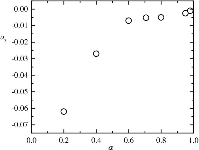
Figure 6: Plot of the simulation values of $a_{3}$ versus $\alpha$ in the case of the Gaussian thermostat.

For $\alpha\geq 0.6$ $|a_{3}|$ remains small, but for larger dissipation the values of $|a_{3}|$ increase rapidly.

The high energy tail predicted by Eq. (42) NE98 ; EP97 is tested in Fig. 7, where

$$G(c)\equiv e^{Ac}\widetilde{f}(\mathbf{c})$$ (71)

is plotted for $\alpha=0.2$ and $\alpha=0.4$. The corresponding values of $A$ are $A\simeq 3.82$ and $A\simeq 4.41$, respectively. The agreement with Eq. (68) is excellent; from the simulation data we can estimate $K\simeq 7$ for $\alpha=0.2$ and $K\simeq 31$ for $\alpha=0.4$.

Figure 7: Plot of the simulation values of the function $G(c)$ defined by Eq. (71) for $\alpha=0.2$ and $\alpha=0.4$ in the case of the Gaussian thermostat. The dashed lines are the Maxwell-Boltzmann predictions.

In this case of a Gaussian thermostat, the overpopulation effect is much more important than in the previous case. At $c=4$, $\widetilde{f}/\phi\simeq 80$ for $\alpha=0.2$ and $\widetilde{f}/\phi\simeq 34$ for $\alpha=0.4$. The results reported here for inelastic hard spheres complement those obtained by Brey et al. BCR99 , where the asymptotic behavior (42) was verified for inelastic hard disks.

Recently, Sela and Goldhirsch SG98 have obtained numerically the function $\Delta(c)$ in the low dissipation limit. In their notation, $\lim_{\alpha\to 1}\Delta(c)\equiv-8\widehat{\Phi}_{\epsilon}(c)$. From simulation results presented in Ref. BMC96 for $\alpha=0.99$ it follows that the function $\widehat{\Phi}_{\epsilon}(c)$ is well represented by the Sonine polynomial $-S_{2}(c^{2})/8$ in the range $0\leq c\leq 1$. However, this agrees only qualitatively with the function $\widehat{\Phi}_{\epsilon}(c)$ obtained numerically by Sela and Goldhirsch SG98 . For instance, from Fig. 3 of Ref. SG98 one gets $\widehat{\Phi}_{\epsilon}(0)\simeq-0.35$, while $-S_{2}(0)/8=-15/64\simeq-0.23$. Moreover, it is claimed in Ref. SG98 that $\widehat{\Phi}_{\epsilon}(c)\sim c^{2}\log c$ for large $c$, which differs from the behavior (42) that has been confirmed here and in Ref. BCR99 . It is possible that the high energy tail obtained from the perturbative approach presented in Ref. SG98 only holds for $1\ll c\ll(1-\alpha^{2})^{-1}$ and thus it is not representative of the general asymptotic behavior for arbitrary $\alpha$.

4.3 Non-Gaussian thermostat

In contrast to the two previous cases, the Sonine polynomials $\{S_{p}(c^{2})\}$ are not expected to constitute a good set for the expansion of the ratio $\widetilde{f}(\mathbf{c})/\phi(\mathbf{c})$ in the case of the non-Gaussian thermostat (15) since the latter is singular at $\mathbf{c}=\mathbf{0}$. Consequently, we do not expect the estimate (50) to be quantitatively accurate. This is confirmed in Fig. 8, where we observe that Eq. (50) gives values that are about 20% smaller in magnitude than the simulation ones.

Figure 8: Plot of the simulation values of $a_{2}$ ($\bigcirc$), $(\mu_{2}-\mu_{2}^{(0)})/\mu_{2}^{(1)}$ ($\bigtriangleup$) and $(\mu_{4}-\mu_{4}^{(0)})/\mu_{4}^{(1)}$ ($\bigtriangledown$) versus $\alpha$ in the case of the non-Gaussian thermostat. The solid and dashed lines are the estimates (50) and (76), respectively.

Also, the approximation (26) with $\mu_{2,4}^{(1)}$ given by Eqs. (28) and (30) is rather poor. It is reasonable to expect that a better approximation would be obtained if $\langle c\rangle$, $\langle c^{3}\rangle$, $\mu_{2}$ and $\mu_{4}$ were computed from the unknown function $\Delta(c)$ rather than from $S_{2}(c^{2})$. When plotting the simulation data of $(\mu_{2}-\mu_{2}^{(0)})/\mu_{2}^{(1)}$, $(\mu_{4}-\mu_{4}^{(0)})/\mu_{4}^{(1)}$, $\langle c\rangle$ and $\langle c^{3}\rangle$ versus $a_{2}$ we have observed that the points fit well in straight lines, as predicted by Eqs. (26), (48) and (49), but with different slopes. More specifically, our simulation results indicate that, instead of Eqs. (26), (48) and (49), one should have (for $d=3$)

$$\mu_{2}\simeq\mu_{2}^{(0)}+\frac{21}{20}\mu_{2}^{(1)}a_{2},$$ (72)

$$\mu_{4}\simeq\mu_{4}^{(0)}+\frac{13}{15}\mu_{4}^{(1)}a_{2},$$ (73)

$$\langle c\rangle\simeq\frac{2}{\pi^{1/2}}\left(1-\frac{3}{2}\frac{1}{8}a_{2}\right),$$ (74)

$$\langle c^{3}\rangle\simeq\frac{2\sqrt{2}}{\pi^{1/2}}\left(1+\frac{23}{20}\frac{3}{8}a_{2}\right).$$ (75)

If we insert the above expressions into Eq.  (44) and neglect terms nonlinear in $a_{2}$, we get

$$a_{2}\simeq-\frac{240(1-\alpha)(1+2\alpha^{2})}{1957-1125\alpha+390(1-\alpha)\alpha^{2}}.$$ (76)

This semi-empirical estimate exhibits a fairly good agreement with the simulation data, as shown in Fig. 8.

The limitations of a Sonine description in the case of the non-Gaussian thermostat are quite apparent in Fig. 9, where $\Delta(c)$ is plotted for $\alpha=0.4$, 0.6 and 0.95. The curves corresponding to $\alpha=0.4$ and $\alpha=0.6$ practically coincide, while the curve corresponding to $\alpha=0.95$ clearly deviates in the region of very small velocities. As a matter of fact, $\Delta(0)$ is roughly equal to $-a_{2}^{-1}$, which indicates an almost vanishing population of rest particles, i.e. $\widetilde{f}(\mathbf{0})\approx 0$, even at $\alpha=0.95$.

Figure 9: Plot of the simulation values of the function $\Delta(c)$ defined by Eq. (45) for $\alpha=0.4$, 0.6 and 0.95 in the case of the non-Gaussian thermostat. The dashed line is the Sonine polynomial $S_{2}(c^{2})$.

A key feature of Fig. 9 is the existence of a non-zero initial slope, $\left.\partial\Delta(c)/\partial c\right|_{c=0}\neq 0$, that cannot be described by any polynomial in $c^{2}$.

From the analysis made at the end of Subsect. 2.3, we expect an underpopulated high energy tail of the form (54), where the coefficient $A$ is unknown. By a fitting of the simulation results we have estimated $A\simeq 1.48$ for $\alpha=0.3$ and $A\simeq 1.51$ for $\alpha=0.4$. Figure 10 shows the function

$$G(c)\equiv e^{Ac^{2}}\widetilde{f}(\mathbf{c})$$ (77)

for $\alpha=0.3$ and $\alpha=0.4$. In both cases the value of $K$ is $K\simeq 1.7$.

Figure 10: Plot of the simulation values of the function $G(c)$ defined by Eq. (77) for $\alpha=0.3$ and $\alpha=0.4$ in the case of the non-Gaussian thermostat. The dashed lines are the Maxwell-Boltzmann predictions.

The regions of small and large velocities are highly underpopulated with respect to the Maxwell-Boltzmann distribution. At $c=3$, for instance, $\widetilde{f}/\phi\simeq 0.12$ for $\alpha=0.3$ and $\widetilde{f}/\phi\simeq 0.10$ for $\alpha=0.4$.

5 Summary and discussion

In this paper we have performed direct Monte Carlo simulations of the Enskog-Boltzmann equation for a fluid of smooth inelastic spheres in spatially uniform states. Upon describing the velocity distribution of the granular fluid by the Enskog-Boltzmann equation (1) it has been implicitly assumed the validity of the “molecular chaos” hypothesis of uncorrelated binary collisions. However, molecular dynamics simulations of hard disks have shown a non-uniform distribution of impact parameters for high enough dissipation ($\alpha<0.8$) Luding . In addition, there exist long range spatial correlations in density and flow fields which cannot be understood on the basis of the Enskog-Boltzmann equation NEBO97 . These two effects are associated with the appearance of the so-called cluster instability BM90 for systems sufficiently large. Since we have simulated directly the spatially uniform equation (1), such an instability is precluded in the simulations.

To compensate for cooling effects associated with the inelasticity of collisions, three types of “thermostatting” external driving forces have been considered. We have analyzed the deviation of the steady-state velocity distribution function from the Maxwell-Boltzmann distribution, as measured by the fourth cumulant $a_{2}$ and by the high energy tail.

A simple mechanism for thermostatting the system is to assume that the particles are subjected to random kicks WM96 , what mimics the effects of shaking or vibrating the vessel ER89 . If this stochastic force has the properties of a white noise [cf. Eq. (8)], it gives rise to a Fokker-Planck diffusion term in the Enskog-Boltzmann equation NE98 . By making a first Sonine approximation, van Noije and Ernst NE98 have obtained an approximate expression for $a_{2}$ as a function of the coefficient of normal restitution $\alpha$. Our simulation results confirm the accuracy of that expression even for large dissipation ($\alpha=0.2$). We have also confirmed a high energy tail of the form $f(\mathbf{v})\sim\exp[-A(v/v_{0})^{3/2}]$ (where $v_{0}$ is the thermal velocity) derived in Ref. NE98 . Moreover, that asymptotic behavior (which represents an overpopulation with respect to the Maxwell-Boltzmann distribution) is already practically reached for $v>4v_{0}$, at least for $\alpha=0.4\mbox{ and }0.5$.

In the absence of any external forcing, the freely evolving granular fluid reaches a homogeneous cooling state in which all the time dependence of the velocity distribution occurs through the thermal velocity $v_{0}(t)$, so that the distribution of the reduced velocity $\mathbf{c}=\mathbf{v}/v_{0}$ is stationary. When the Enskog-Boltzmann equation is written in terms of this reduced velocity, the operator $\partial/\partial t$ gives rise to an operator that coincides with the one representing the action of an external force proportional to the particle velocity [cf. Eq. (12)]. This type of “anti-drag” force can also be justified by Gauss’s principle of least constraint EM90 and has been widely used in nonequilibrium molecular dynamics simulations of molecular fluids. Thus, the homogeneous cooling state is equivalent to the steady state reached under a Gaussian thermostat. In their simulations, Brey et al. BMC96 ; BCR99 used the former point of view, while in this paper we have used the latter. Our simulations complement those of Ref. BMC96 also in that we have considered a wide range $0.2\leq\alpha\leq 1$, while Brey et al. BMC96 analyzed in detail the region $0.7\leq\alpha\leq 1$. They obtained an excellent agreement with the estimate (5) based on a Sonine approximation, first derived in Ref. NE96 . However, as $\alpha$ decreases and $a_{2}$ becomes larger, we have seen in this paper that Eq. (5) overestimates $a_{2}$. This discrepancy can be traced back to contributions associated with higher order Sonine polynomials as well as to the ambiguity involved in the approximate determination of $a_{2}$ by neglecting nonlinear terms in the exact equation (38). If Eq.  (38) is rewritten in another equivalent form (for example, by transferring a quantity from one side to the other), the same method yields a different approximation for $a_{2}$. As long as $a_{2}$ remains small (say $|a_{2}|<0.05$), all the approximations give practically undistinguishable results. On the other hand, for larger values of $a_{2}$ (i.e., for $\alpha<0.5$) the result is relatively dependent of the route followed. By starting from Eq. (38) rewritten as $\mu_{4}/(1+a_{2})=(d+2)\mu_{2}$, we have obtained the estimate (40), which is seen to agree fairly well with the simulation results for the whole range of coefficients of restitution considered. The asymptotic analysis of the kinetic equation predicts a high energy tail of the form NE98 ; EP97 $f(\mathbf{v})\sim\exp[-A(v/v_{0})]$, what represents an overpopulation phenomenon stronger than in the previous case. This behavior was already confirmed in Ref. BCR99 for $d=2$ and has now been confirmed by our simulation results for $d=3$.

In the case of the Gaussian thermostat, the heating force points in the motion direction and its magnitude is proportional to that of the particle velocity. This is a very efficient thermostat because it gives more energy to fast particles, which are the ones colliding more frequently. In contrast, the stochastic thermostat adds a velocity increment per unit of time that is random both in direction and in magnitude. This is why the high energy population is larger with the Gaussian thermostat than with the stochastic thermostat. Nevertheless, in both cases such a population is larger than in the case of elastic particles at equilibrium. One could be tempted to expect that this overpopulation is a common feature of heated granular fluids, regardless of the mechanism of heating. Our third choice of thermostat, Eq. (14), proves that this is not the case. Like in the case of the stochastic thermostat, the force is independent of the magnitude of the particle velocity; like in the case of the Gaussian thermostat, the force is deterministic and points in the motion direction. The action of this third thermostat can be graphically described by saying that, between two successive collisions, a particle feels a “pseudo-gravity” field that makes it to “fall” along its motion direction. With this choice of a non-Gaussian deterministic thermostat, the Sonine polynomials $\{S_{p}(c^{2})\}$ are not a good set to represent the ratio $\widetilde{f}(\mathbf{c})/\phi(\mathbf{c})$, even for low dissipation. As a consequence, the theoretical estimate of $a_{2}$ derived by assuming that $[\widetilde{f}(\mathbf{c})/\phi(\mathbf{c})-1]/a_{2}\equiv\Delta(c)\simeq S_{2}(c^{2})$, while being qualitatively correct, is not quantitatively accurate. We have not been able to get the functional form of $\Delta(c)$ in the limit of low dissipation. However, we have estimated its contributions to $\langle c\rangle$, $\langle c^{3}\rangle$, $\mu_{2}$ and $\mu_{4}$ from the simulation data. This has allowed us to obtain an approximate expression for $a_{2}$ that fits well the simulation results. An interesting feature of the velocity distribution function in this case is that it is highly underpopulated with respect to the Maxwell-Boltzmann distribution both for small and large velocities. Between two successive collisions, every particle experiences a constant tangential acceleration $g$. The total work done by this force is exactly compensated by the total loss of energy through collisions, which are much more frequent for fast particles than for slow ones. Therefore, the population of slow particles decreases because of the action of the external force, while that of fast particles decreases because of the effect of collisions. The high energy tail of the distribution function is of the form $\widetilde{f}(\mathbf{c})\sim\exp(-Ac^{2})$ with $A>1$. In this case the gain and loss terms of the collision integral are comparable, so that the dependence of $A$ on $\alpha$ is an open problem.

Appendix A Collisional moments

In this Appendix we derive the expressions (64)–(3). Starting from Eq. (22) and by a standard change of variables, it is easy to get NE98

$$\mu_{p}=\int d\mathbf{c}_{1}\int d\mathbf{c}_{2}\,\widetilde{f}(\mathbf{c}_{1})\widetilde{f}(\mathbf{c}_{2})\widetilde{\Phi}_{p}(\mathbf{c}_{1},\mathbf{c}_{2}),$$ (78)

where

$$\widetilde{\Phi}_{p}(\mathbf{c}_{1},\mathbf{c}_{2})=\frac{1}{2}\int d\widehat{\boldsymbol{\sigma}}\,\Theta(\mathbf{c}_{12}\cdot\widehat{\boldsymbol{\sigma}})(\mathbf{c}_{12}\cdot\widehat{\boldsymbol{\sigma}})\left[c_{1}^{p}+c_{2}^{p}-{c_{1}^{\prime}}^{p}-{c_{2}^{\prime}}^{p}\right],$$ (79)

with $\mathbf{c}_{1,2}^{\prime}=\mathbf{c}_{1,2}\mp\frac{1}{2}(1+\alpha)(\mathbf{c}_{12}\cdot\widehat{\boldsymbol{\sigma}})\widehat{\boldsymbol{\sigma}}$. In the cases $p=2$ and $p=4$ we have

$$c_{1}^{2}+c_{2}^{2}-{c_{1}^{\prime}}^{2}-{c_{2}^{\prime}}^{2}=\frac{1-\alpha^{2}}{2}(\mathbf{c}_{12}\cdot\widehat{\boldsymbol{\sigma}})^{2},$$ (80)

$$c_{1}^{4}+c_{2}^{4}-{c_{1}^{\prime}}^{4}-{c_{2}^{\prime}}^{4} = (1-\alpha^{2})(\mathbf{c}_{12}\cdot\widehat{\boldsymbol{\sigma}})^{2}\left(\frac{c_{12}^{2}}{4}+C_{12}^{2}\right)$$ (81)

$$-\frac{(1-\alpha^{2})^{2}}{8}(\mathbf{c}_{12}\cdot\widehat{\boldsymbol{\sigma}})^{4}$$

$$-2(1+\alpha)^{2}(\mathbf{c}_{12}\cdot\widehat{\boldsymbol{\sigma}})^{2}(\mathbf{C}_{12}\cdot\widehat{\boldsymbol{\sigma}})^{2}$$

$$+4(1+\alpha)(\mathbf{c}_{12}\cdot\widehat{\boldsymbol{\sigma}})(\mathbf{C}_{12}\cdot\widehat{\boldsymbol{\sigma}})$$

$$\times(\mathbf{c}_{12}\cdot\mathbf{C}_{12}),$$

where $\mathbf{c}_{12}=\mathbf{c}_{1}-\mathbf{c}_{2}$, $\mathbf{C}_{12}=\frac{1}{2}(\mathbf{c}_{1}+\mathbf{c}_{2})$. Consequently,

$$\widetilde{\Phi}_{2}(\mathbf{c}_{1},\mathbf{c}_{2})=\frac{\beta_{3}(1-\alpha^{2})}{4}c_{12}^{3},$$ (82)

$$\widetilde{\Phi}_{4}(\mathbf{c}_{1},\mathbf{c}_{2}) = \beta_{3}c_{12}\left\{\frac{(d+2)(1-\alpha^{2})}{2d}c_{12}^{2}C_{12}^{2}\right.$$ (83)

$$+\frac{(1-\alpha^{2})(d+1+2\alpha^{2})}{8(d+3)}c_{12}^{4}$$

$$+\frac{(2d+3-3\alpha)(1+\alpha)}{d+3}$$

$$\left.\times\left[\left(\mathbf{c}_{12}\cdot\mathbf{C}_{12}\right)^{2}-\frac{1}{d}c_{12}^{2}C_{12}^{2}\right]\right\},$$

where we have taken into account that

$$\int d\widehat{\boldsymbol{\sigma}}\,\Theta(\widehat{\mathbf{c}}\cdot\widehat{\boldsymbol{\sigma}})(\widehat{\mathbf{c}}\cdot\widehat{\boldsymbol{\sigma}})^{n}=\pi^{(d-1)/2}\frac{\Gamma((n+1)/2)}{\Gamma((n+d)/2)}\equiv\beta_{n},$$ (84)

$$\int d\widehat{\boldsymbol{\sigma}}\,\Theta(\widehat{\mathbf{c}}\cdot\widehat{\boldsymbol{\sigma}})(\widehat{\mathbf{c}}\cdot\widehat{\boldsymbol{\sigma}})^{n}\widehat{\boldsymbol{\sigma}}=\beta_{n+1}\widehat{\boldsymbol{c}},$$ (85)

$$\int d\widehat{\boldsymbol{\sigma}}\,\Theta(\widehat{\mathbf{c}}\cdot\widehat{\boldsymbol{\sigma}})(\widehat{\mathbf{c}}\cdot\widehat{\boldsymbol{\sigma}})^{n}\widehat{\boldsymbol{\sigma}}\widehat{\boldsymbol{\sigma}}=\frac{\beta_{n}}{n+d}\left(n\widehat{\boldsymbol{c}}\widehat{\boldsymbol{c}}+\mathsf{I}\right).$$ (86)

In the three-dimensional case, Eqs. (78), (82) and (83) yield Eqs. (64)–(3).

References

- (1) C. S. Campbell, Ann. Rev. Fluid Mech. 22, 57 (1990).
- (2) J. J. Brey, J. W. Dufty and A. Santos, J. Stat. Phys. 87, 1051 (1997); T. P. C. van Noije, M. H. Ernst and R. Brito, Physica A 251, 266 (1998).
- (3) A. Goldshtein and M. Shapiro, J. Fluid Mech. 282, 75 (1995).
- (4) T. P. C. van Noije and M. H. Ernst, internal report, Institute for Theoretical Physics, Universiteit Utrecht, 1996.
- (5) T. P. C. van Noije and M. H. Ernst, Gran. Matt. 1, 57 (1998).
- (6) J. J. Brey, M. J. Ruiz-Montero and D. Cubero, Phys. Rev. E 54, 3664 (1996).
- (7) V. Garzó and J. W. Dufty, Phys. Rev. E 60, 5706 (1999).
- (8) S. E. Esipov and T. Pöschel, J. Stat. Phys. 86, 1385 (1997).
- (9) J. J. Brey, D. Cubero and M. J. Ruiz-Montero, Phys. Rev. E 59, 1256 (1999).
- (10) P. Evesque and J. Rajchenbach, Phys. Rev. Lett. 62, 44 (1989); Y-h. Taguchi, Phys. Rev. Lett. 69, 1367 (1992); J. A. C. Gallas, H. J. Herrmann and S. Sokołowski, Phys. Rev. Lett. 69, 1371 (1992).
- (11) K. Ichiki and H. Hayakawa, Phys. Rev. E 52, 658 (1995); 57, 1990 (1998).
- (12) D. R. M. Williams and F. C. MacKintosh, Phys. Rev. E 54, R9 (1996); D. R. M. Williams, Physica A 233, 718 (1996); M. R. Swift, M. Boamfǎ, S. J. Cornell and A. Maritan, Phys. Rev. Lett. 80, 4410 (1998).
- (13) D. J. Evans and G. P. Morriss, Statistical Mechanics of Nonequilibrium Liquids (Academic Press, London, 1990).
- (14) V. Garzó, A. Santos and J. J. Brey, Physica A 163, 651 (1990).
- (15) J. W. Dufty, A. Santos, J. J. Brey and R. F. Rodríguez, Phys. Rev. A 33, 459 (1986); A. Santos and V. Garzó, Physica A 213, 409 (1995).
- (16) G. Bird, Molecular Gas Dynamics and the Direct Simulation of Gas Flows (Clarendon Press, Oxford, 1994).
- (17) J. M. Montanero and A. Santos, Phys. Rev. E 54, 438 (1996); Phys. Fluids 9, 2057 (1997).
- (18) J. M. Montanero, V. Garzó, A. Santos and J. J. Brey, J. Fluid Mech. 389, 391 (1999).
- (19) G. Peng and T. Ohta, Phys. Rev. E 58, 4737 (1998).
- (20) N. Sela and I. Goldhirsch, J. Fluid Mech. 361, 41 (1998).
- (21) S. Luding, M. Müller and S. McNamara, “The validity of ‘molecular chaos’ in granular flows”, in: World Congress on Particle Technology (Brighton, 1998, CD: ISBN 0-85295-401-9); S. Luding, T.A.S.K. Quarterly, Scientific Bulletin of the Academic Computer Centre of the Technical University of Gdansk 2, 417 (1998), and cond-mat/9810116.
- (22) T. P. C. van Noije, M. H. Ernst, R. Brito and J. A. G. Orza, Phys. Rev. Lett. 79, 411 (1997); T. P. C. van Noije, R. Brito and M. H. Ernst, Phys. Rev. E 57, R4891 (1998); T. P. C. van Noije, M. H. Ernst, E. Trizac and I. Pagonabarraga, Phys. Rev. E 59, 4326 (1999).
- (23) B. Bernu and R. Mazighi, J. Phys. A 23, 5745 (1990); S. M. McNamara and W. R. Young, Phys. Fluids A 5, 34 (1993); Phys. Rev. E 50, R28 (1994); I. Goldhirsch and G. Zanetti, Phys. Rev. Lett. 70, 1619 (1993); N. Sela and I. Goldhirsch, Phys. Fluids 7, 507 (1995).