Conductivity of a clean one-dimensional wire

Abstract

We study the low-temperature low-frequency conductivity $\sigma$ of an interacting one dimensional electron system in the presence of a periodic potential. The conductivity is strongly influenced by conservation laws, which, we argue, need be violated by at least two non-commuting Umklapp processes to render $\sigma$ finite. The resulting dynamics of the slow modes is studied within a memory matrix approach, and we find exponential increase as the temperature is lowered, $\sigma\sim(\Delta n)^{2}e^{T_{0}/(NT)}$ close to commensurate filling $M/N$, $\Delta n=n-M/N\ll 1$, and $\sigma\sim e^{(T^{\prime}_{0}/T)^{2/3}}$ elsewhere.

The finite-temperature conductivity of a clean one-dimensional wire [1] is a fundamental and much studied question. Clearly the “bulk” conductivity of a wire in the absence of a periodic potential is infinite even at finite temperatures $T$. In this case the conductance is independent of the length of the wire and is determined by the contacts only. Surprisingly, much less is known about the conductivity in the presence of Umklapp scattering induced by a periodic potential. There is not even an agreement whether it is finite or infinite at finite temperatures for generic systems [2, 3, 4, 5, 6]. We shall show that the correct answer emerges when all relevant (weakly violated) conservation laws are taken into account. Those conservation laws are exact at the Fermi surface and are violated by Umklapp terms away from it. We shall study the associated slow modes by means of a memory matrix formalism able to keep track of their dynamics. It will allow us to calculate reliably the low temperature, low frequency conductivity.

The topology of the Fermi surface of a $1d$ metal determines its low-energy excitations. Two well defined Fermi-points exist at momenta $k=\pm k_{F}$, allowing us to define left and right moving excitations, to be described by $\Psi_{L/R,\sigma=\uparrow\downarrow}$. We shall include in the fields momentum modes extending to the edge of the Brillouin zone, usually omitted in treatments that concentrate on physics very close to the Fermi-surface.

The Hamiltonian, including high energy processes, is

$$H=H_{LL}+H_{\text{irr}}+\sum_{n,m}^{\infty}H_{n,m}^{U}.$$ (1)

$H_{LL}$ is the well-known Luttinger liquid Hamiltonian capturing the low energy behavior[1],

$$H_{LL} = v_{F}\int\left(\Psi_{L\sigma}^{\dagger}i\partial_{x}\Psi_{L\sigma}-\Psi_{R\sigma}^{\dagger}i\partial_{x}\Psi_{R\sigma}\right)+g\int\rho(x)^{2}$$ (2)

$$= \frac{1}{2}\int\frac{dx}{2\pi}\sum_{\nu=\sigma,\rho}v_{\nu}\left(K_{\nu}(\partial_{x}\theta_{\nu})^{2}+\frac{1}{K_{\nu}}(\partial_{x}\phi_{\nu})^{2}\right)$$ (3)

$v_{F}$ is the Fermi velocity, $g>0$ measures the strength of interactions, $\rho=\rho_{L}+\rho_{R}$ is the sum of the left and right moving electron densities. In the second line we wrote the bosonized[1] version of the Hamiltonian. Here $v_{\sigma}$, $v_{\rho}$ are the spin and charge velocities, and the interactions determine the Luttinger parameters $K_{\nu}$ with $v_{\nu}K_{\nu}=v_{F}$, $v_{\rho}/K_{\rho}=v_{F}+g/\pi$, $v_{\sigma}/K_{\sigma}=v_{F}-g/\pi$.

The high energy processes are captured in the subsequent terms which are formally irrelevant at low energies (we consider only systems away from a Mott transition, i.e. away from half filling). Some of them, however, determine the low-frequency behavior of the conductivity at any finite $T$, since they induce the decay of the conserved modes of $H_{LL}$ (they are “dangerously irrelevant”). We classify these irrelevant terms with the help of two operators which will play the central role in our discussion. The first one is the translation operator $P_{T}$ of the right- and left-moving fields, the second one, $J_{0}=N_{R}-N_{L}$, is the difference of the number of right- and left-moving electrons, and is up to $v_{F}$, the charge current of $H_{LL}$:

$$P_{T} = \sum_{\sigma}\int dx\left(\Psi_{R\sigma}^{\dagger}(-i\partial_{x})\Psi_{R\sigma}+\Psi_{L\sigma}^{\dagger}(-i\partial_{x})\Psi_{L\sigma}\right)$$ (4)

$$J_{0} = N_{R}-N_{L}=\sum_{\sigma}\int dx\left(\Psi_{R\sigma}^{\dagger}\Psi_{R\sigma}-\Psi_{L\sigma}^{\dagger}\Psi_{L\sigma}\right)$$ (5)

Both $P_{T}$ and $J_{0}$ are conserved by $H_{LL}$; their importance for transport properties is due to the fact that both stay approximately conserved in any one dimensional metal (away from half filling): processes which change $J_{0}$ are forbidden close to the Fermi surface by momentum conservation. The linear combination $P_{0}=P_{T}+k_{F}J_{0}$ can be identified with the total momentum of the full Hamiltonian $H$ and is therefore also approximately conserved.

We proceed to the classification of the formally irrelevant terms in the Hamiltonian. This classification allows us to select all those terms (actually few in number) that determine the current dynamics. $H_{\text{irr}}$ includes all terms in $H-H_{LL}$ which commute with both $P_{T}$ and $J_{0}$, such as corrections due to the finite band curvature, due to finite-range interactions and similar terms. We will not need their explicit form.

The Umklapp terms $H^{U}_{n,m}$ ($n,m=0,1,...$) convert $n$ right-movers to left-movers (and vice versa) picking up lattice momentum $m2\pi/a=mG$, and do not commute with either $P_{T}$ or $J_{0}$. Leading terms are of the form,

$$H^{U}_{0,m} \approx g^{U}_{0,m}\int e^{i\Delta k_{0,m}x}(\rho_{L}+\rho_{R})^{2}+h.c.$$ (6)

$$H^{U}_{1,m} \approx g^{U}_{1,m}\sum_{\sigma}\int e^{i\Delta k_{1,m}x}\Psi^{\dagger}_{R\sigma}\Psi_{L\sigma}\rho_{-\sigma}+h.c.$$ (7)

$$H^{U}_{2,m} \approx g^{U}_{2,m}\int e^{i\Delta k_{2,m}x}\Psi^{\dagger}_{R\uparrow}\Psi^{\dagger}_{R\downarrow}\Psi_{L\downarrow}\Psi_{L\uparrow}+h.c.$$ (8)

with momentum transfer $\Delta k_{n,m}=n2k_{F}-mG$. A process transfering $n>1$ electrons with total spin $n_{s}/2$ pointing in the $z$-direction can be neatly expressed as

$$H^{U}_{n,m}=\frac{g^{U}_{n,m,n_{s}}}{(2\pi\alpha)^{n}}\int e^{i\Delta k_{n,m}x}e^{i\sqrt{2}(n\phi_{\rho}+n_{s}\phi_{\sigma})}+h.c.,$$ (9)

$\alpha$ being a cut-off, of the order of the lattice spacing. In fermionic variables the integrand takes the form $\prod_{j=0}^{n/2-1}\Psi_{R\uparrow}^{\dagger}(x+j\alpha)\Psi_{R\downarrow}^{\dagger}(x+j\alpha)\Psi_{L\downarrow}(x+j\alpha)\Psi_{L\uparrow}(x+j\alpha)$ (for $n_{s}=0$ and even $n$).

Note, though, that any single term $H^{U}_{nm}$ conserves a linear combination of $J_{0}$ and $P_{T}$,

$$\left[H^{U}_{nm},\Delta k_{nm}J_{0}+2nP_{T}\right]=0.$$ (10)

Indeed, a term of the form (9) would appear in a continuum model without Umklapp scattering, but with a Fermi momentum $\tilde{k}_{F}=\Delta k_{nm}/(2n)$. In such a model, $\Delta k_{nm}J_{0}/(2n)+P_{T}$ is the total momentum of the system and therefore conserved. The importance of this simple but essential conservation law has to our knowledge not been sufficiently realized in previous calculations of the conductivity. Due to this conservation law a single Umklapp term can never induce a finite conductivity! At least two independent Umklapp terms are required to lead to a complete decay of the current. Further, two incommensurate Umklapp terms suffice to generate the rest.

To calculate the conductivity it is necessary to keep track of the nearly conserved quantities and their relation to the current. We will develop a description of the slowest variables using the Mori-Zwanzig memory functional [7, 8, 2]. Approximations within this scheme amount to short-time expansions. In general, the short time decay of a quantity carries little information on its long-time behavior; this, however, is not the case for the slowest variables in the system, where the short time and hydrodynamic behavior coincide.

To set up the formalism [7] we define a scalar product $(A|B)$ in the space of operators,

$$\left(A(t)|B\right) \equiv \frac{1}{\beta}\int_{0}^{\beta}d\lambda\left\langle A(t)^{\dagger}B(i\lambda)\right\rangle,$$ (11)

where we use the usual Heisenberg picture with $A(t)=e^{iHt}Ae^{-iHt}$. We choose a set “slow” operators $j_{1},j_{2},...j_{N}$ which includes $j_{1}=J$, the full current operator. Standard arguments [7] lead to the electric conductivity,

$$\sigma(\omega,T) = \left[\left(\hat{M}(\omega,T)-i\omega\right)^{-1}\hat{\chi}(T)\right]_{11}.$$ (12)

Here $\hat{\chi}_{pq}=\beta(j_{p}|j_{q})$ is the matrix of the static $j_{p}j_{q}$ susceptibilities (as usually defined), and $\hat{M}$ is the matrix of memory functions given by the projected correlation functions of time-derivatives of the “slow” operators,

$$\hat{M}_{pq}(\omega)=\beta\sum_{r}\left(\partial_{t}j_{q}\left|Q\frac{i}{\omega-QLQ}Q\right|\partial_{t}j_{r}\right)(\hat{\chi}^{-1})_{rp}.$$ (13)

The Liouville “super”-operator, $L$, is defined by $LA=[H,A]$ and $Q$ is the projection operator on the space perpendicular to the slowly varying variables $j_{p}$,

$$Q=1-\sum_{pq}|j_{q})\beta(\hat{\chi}^{-1})_{qp}(j_{p}|.$$ (14)

We assumed for simplicity that all $j_{p}$ have the same signature under time reversal.

The perturbative expansion of the memory matrix $\hat{M}$ is accompanied by factors $1/\omega$ guaranteeing it is always valid at short times. It is also valid for small frequencies provided the slowly evolving degrees of freedom are projected out (by the operator $Q$). Unlike the conductivity it is expected to be a smooth function of the coupling constants which can be perturbatively evaluated.

We first consider a situation where some linear combinations of the $j_{p}$ are conserved by $H$, in which case an infinite conductivity is expected. We introduce ${\cal P}_{c}$, the projection operator on the space of conserved currents, and carry out the required matrix inversion to find,

$$\sigma(\omega\to 0,T>0) = \sigma_{\text{reg}}(\omega,T)+i\frac{(\hat{\chi}\hat{\chi}_{c}^{-1}\hat{\chi})_{11}}{\omega+i0},$$ (15)

where $\hat{\chi}_{c}^{-1}={\cal P}_{c}({\cal P}_{c}\hat{\chi}{\cal P}_{c})^{-1}{\cal P}_{c}$. Within any simple (short-time) approximation, $\sigma_{\text{reg}}(\omega,T)$ as defined above, is regular (this approximation fails e.g. if some conserved current $\hat{j}$ is not included in $j_{1}...j_{N}$). Hence the Drude weight $D(T)$ is finite at finite temperatures, $\text{Re}\sigma(\omega\to 0)=2\pi D(T)\delta(\omega)=\pi(\hat{\chi}\hat{\chi}_{c}^{-1}\hat{\chi})_{11}\delta(\omega)$. It is determined by the “overlap” of the physical current operator $J$ with the conserved quantities $\chi_{1s}$, $s$ labeling the conserved currents. Remarkably, our perturbative approximation is in accord with an exact inequality [5] for the Drude weight, $D(T)\geq\frac{1}{2}(\hat{\chi}\hat{\chi}_{c}^{-1}\hat{\chi})_{11}$. Note that $\hat{\chi}$ can be calculated to an arbitrary degree of precision around a Luttinger liquid and that the lower bound can be improved by including more conserved quantities [5].

Now consider the more realistic situation where the previously conserved currents decay slowly (via Umklapp processes), in which case a finite conductivity is expected. We restrict ourselves to the two-dimensional space spanned by $v_{F}J_{0}$ and $P_{T}$, which we argue have the longest decay rate and dominate the transport. Here we approximate $J\approx v_{F}J_{0}$ to keep the presentation simple. This affects only the high frequency behavior of the conductivity [3]. There is a large number of other nearly conserved quantities. For example $H_{LL}+H^{U}_{21}$, the relevant low-energy model close to half filling, is integrable and therefore is characterized by an infinite number of conservation laws. We can, however, neglect them at low $T$ if our initial model is not integrable, expecting that practically all conservation laws are destroyed by (formally irrelevant) terms close to the Fermi surface leading to decay rates proportional to some power of $T$. This is to be compared to $J_{0}$ and $P_{T}$ which commute with all scattering processes at the Fermi surface, leading to exponentially large lifetimes.

We now proceed to calculate the Memory matrix. To leading order in the perturbations we can replace $L$ in (13) by $L_{LL}=[H_{LL},.]$ [9], since $\partial_{t}v_{F}J_{0}$ and $\partial_{t}P_{T}$ are already linear in $g^{U}_{n,m}$. As $L_{LL}P_{T}=L_{LL}J_{0}=0$, there is no contribution from the projection operator $Q$. The memory matrix takes the form,

$$\hat{M} \approx \sum_{nm}M_{nm}(\omega,T)\left(\begin{array}[]{cc}v_{F}^{2}(2n)^{2}&-2nv_{F}\Delta k_{nm}\\ -2nv_{F}\Delta k_{nm}&(\Delta k_{nm})^{2}\end{array}\right)\hat{\chi}^{-1}$$ (18)

where,

$$\hat{\chi} \approx \left(\begin{array}[]{cc}2v_{F}/\pi&0\\ 0&\frac{\pi T^{2}}{3}\left(\frac{1}{v_{\rho}^{3}}+\frac{1}{v_{\sigma}^{3}}\right)\end{array}\right)$$ (21)

$$M_{nm} \equiv (g^{U}_{nm})^{2}M_{n}(\Delta k_{n,m},\omega)\equiv\frac{\langle F;F\rangle^{0}_{\omega}-\langle F;F\rangle^{0}_{\omega=0}}{i\omega}.$$ (22)

Here $F=[J_{0},H^{U}_{nm}]/(2n)$ (for simplicity we drop the indices $n,m$ on F), and $\langle F;F\rangle^{0}_{\omega}$ is the retarded correlation function of $F$ calculated with respect to $H_{LL}$.

The memory function $M_{2}$ of the $4k_{F}-Q$ process $H^{U}_{21}$ was calculated by Giamarchi [2], (not considering the matrix structure of $\hat{M}$ required by the conservation laws.) Higher Umklapps are considered in [3]. For $n_{s}=0$ and even $n$ the memory function due to the term (9) can be analytically calculated,

$$M_{n}(\Delta k,\omega)= \frac{2\sin 2\pi K^{n}_{\rho}}{\pi^{4}\alpha^{2n-2}v_{\rho}}\left[\frac{2\pi\alpha T}{v_{\rho}}\right]^{4K^{n}_{\rho}-2}\frac{1}{i\omega}\times$$ (23)

$$\times[B(K^{n}_{\rho}- iS_{+},1-2K^{n}_{\rho})B(K^{n}_{\rho}-iS_{+},1-2K^{n}_{\rho})$$ (24)

$$-B(K^{n}_{\rho}- iS_{+}^{0},1-2K^{n}_{\rho})B(K^{n}_{\rho}-iS_{+}^{0},1-2K^{n}_{\rho})]$$ (26)

$$\approx\frac{\alpha^{2-2n}}{\pi^{2}\Gamma^{2}(2K^{n}_{\rho})v_{\rho}T}\left(\frac{\alpha\Delta k}{2}\right)^{4K_{\rho}^{n}-2}e^{-v_{\rho}\Delta k/(2T)}$$

where $K^{n}_{\rho}=(n/2)^{2}K_{\rho}$, $B(x,y)=\Gamma(x)\Gamma(y)/\Gamma(x+y)$ and $S_{\pm}=(\omega\pm v_{\rho}\Delta k)/(4\pi T)$, $S_{\pm}^{0}=S_{\pm}(\omega=0)$. The last line is valid for $\omega=0$ and $T\ll v_{\rho}\Delta k$.

The origin of the exponential factor is as follows: processes involving momentum transfer $\Delta k$ are associated with initial and final states of energies $v|\Delta k|/2$, which are exponentially suppressed. If only charge degrees of freedom are involved $v=v_{\rho}$, otherwise $v=\text{min}(v_{\sigma},v_{\rho})=v_{\sigma}$ [9]. For $T\ll v_{\sigma}\Delta k_{nm}$, $n_{s}>0$ and $\omega=0$, we have,

$$M_{n}(\Delta k)\sim\frac{\left(\alpha T/v_{\rho}\right)^{n^{2}K_{\rho}-1}\left(\alpha\Delta k\right)^{n_{s}^{2}K_{\sigma}-2}}{\Gamma^{2}(n_{s}^{2}K_{\sigma}/2)v_{\sigma}^{2}\alpha^{2n-3}}e^{-v_{\sigma}\Delta k/(2T)},$$ (27)

while for $T\gg v_{\rho}\Delta k_{nm}$: $M_{n}\sim T^{n^{2}K_{\rho}+n_{s}^{2}K_{\sigma}-3}$.

Using the above expressions with only one Umklapp term leads to a finite Drude weight (cf eq(15)),

$$D(T)\approx\frac{v_{\rho}K_{\rho}}{\pi}\frac{1}{1+T^{2}\frac{2\pi^{2}n^{2}K_{\rho}}{3(v_{\rho}\Delta k_{nm})^{2}}\left(1+\frac{v_{\rho}^{3}}{v_{\sigma}^{3}}\right)}.$$ (28)

in accord with the observation that one process $H^{U}_{nm}$ is not sufficient to degrade the current.

FIG. 1.: The low frequency behavior of $\sigma(\omega)$ in the presence of two Umklapp terms for two different $T$. The dashed lines are the result one obtains in conventional perturbation theory neglecting [2] the matrix structure of $\hat{M}$ and the related conservation laws. ($g_{20}=g_{21}=1$, $K_{\rho}=0.7$, $K_{\sigma}=1.3$, $\Delta k_{21}=-1.5\Delta k_{20}$, thick lines $T=0.2$, thin lines $T=0.18$, $\omega$ and $T$ measured in units of $v_{\rho}\Delta k_{20}$). Note that two time scales appear - each describing the scale on which the associated conservation law is violated. The inset displays the $T$ dependence of $\sigma(\omega=0)$.

Only in the presence of a second incommensurate process $H^{U}_{n^{\prime}m^{\prime}}$ is the dc conductivity finite,

$$\sigma(T,\omega=0)=\frac{(\Delta k_{nm})^{2}/M_{n^{\prime}m^{\prime}}+(\Delta k_{n^{\prime}m^{\prime}})^{2}/M_{nm}}{\pi^{2}(n\Delta k_{n^{\prime}m^{\prime}}-n^{\prime}\Delta k_{nm})^{2}}$$ (29)

Note that the slowest process determines the low-$T$ conductivity. The frequency and temperature dependence of the conductivity in the case of two competing Umklapp terms is shown in Fig. 1.

The commensurate situation $\Delta k_{nm}=0$ requires extra considerations. Whether the dominant scattering process $H_{nm}$ will completely relax the current $J$ depends according to (15) on the overlap $\chi_{JP_{T}}$ ($[P_{T},H_{nm}]=0$). Using the continuity equation for the charge, $\chi_{JP_{T}}$ can be related to the deviation $\Delta\rho=2\Delta n/a$ of the electron density from commensurate filling with the remarkable identity $\chi_{JP_{T}}=2\Delta n/a+O(e^{-\beta\epsilon_{F}})$. In a 3d lattice of 1d wires, $\Delta n$ is fixed by charge neutrality and is $T$ independent, in a single wire with contacts $\Delta n$ varies at low $T$ with $\Delta n(T)\sim T^{2}/(mv^{3})$, where the mass $m$ is a measure of the breaking of particle-hole symmetry, e.g. due to a band-curvature $k^{2}/2m$. In this case it is important to replace $\Delta k_{nm}=0$ in Eqn. (28) or (29) by $G\Delta n(T)$.

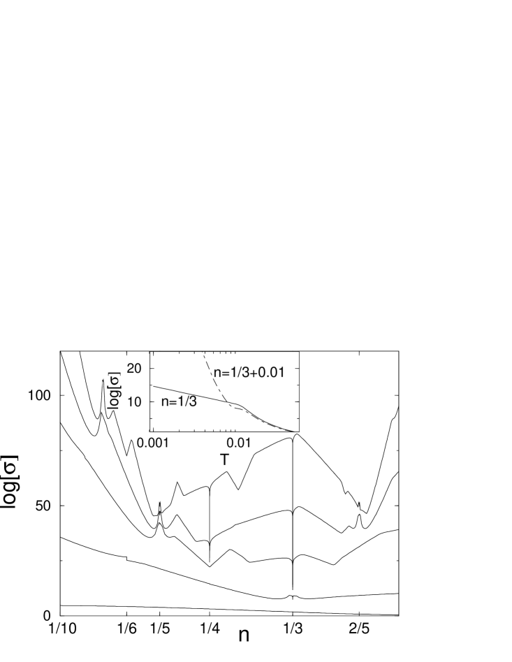
FIG. 2.: Schematic plot of $\log[\sigma]$ as a function of the filling $n=2k_{F}/G$ for various temperatures ($vG\beta=30,100,300,500,800$) based on an asymptotic (eqn.(27)) evaluation of (12). Near commensurate fillings $n_{c}$ the conductivity is strongly enhanced at low temperatures but drops at $n=n_{c}$. The inset displays the $T$-dependence of $\sigma$ for $n=1/3$ and a filling very close to $1/3$ (dashed line).

Which of the various scattering processes will eventually dominate at lowest $T$? At intermediate temperatures, certainly low-order (small $n$) scattering events win, being less suppressed by Pauli blocking. At lower temperature the exponential factors in (27) prevail and the processes with the smallest $\Delta k_{nm}$ are favored. We first analyze the situation close to a commensurate point $k_{F}\approx GM_{0}/(2N_{0})$. The two dominant processes are $H^{U}_{N_{0}M_{0}}$ with $\Delta k_{N_{0}M_{0}}\approx 0$ and $H^{U}_{N_{1}M_{1}}$ with $\Delta k_{N_{1}M_{1}}=\pm G/N_{0}$ (or $N_{1}M_{0}=\pm 1\text{ mod }N_{0}$). The integer $N_{1}$ of order $N_{0}$, $N_{1}=\gamma_{1}N_{0}$, depends strongly on the precise values of $N_{0}$ and $M_{0}$. We thus find that the d.c. conductivity at low $T$ is largest close to commensurate points with,

$$\sigma(k_{F}\approx GM_{0}/(2N_{0}))\sim(\Delta n(T))^{2}\exp[\beta vG/(2N_{0})]$$ (30)

but $\sigma\sim T^{-N_{0}^{2}K_{\rho}-(N_{0}\text{ mod }2)^{2}K_{\sigma}+3}$ if the density is exactly commensurate with $|\Delta n(T)|<e^{-\beta Gv/(4N_{0})}$.

To estimate the conductivity at a typical “incommensurate” point or at commensurate points at temperatures not too low, we have to balance algebraic and exponential suppression in (27) by minimizing $-\beta vG/(2N)+(\gamma_{1}N)^{2}K\log[T]$ in a saddle-point approximation to the sum over all Umklapp processes in ${\hat{M}}$. Up to logarithmic corrections we obtain $N_{\text{max}}^{3}\sim\beta vG/(\gamma_{1})^{2}$ and therefore for a “typical” incommensurate filling,

$$\sigma_{\text{typical}}\sim\exp[c(\beta vG)^{2/3}]$$ (31)

where $c$ is a number depending logarithmically on $T$. At present we cannot rule out that various logarithmic corrections sum up to modify the power law in the exponent. We argue, however, that due to the exponential increase (30) of $\sigma$ at commensurate fillings with exponents proportional to $1/N_{0}$, the conductivity at small $T$ at any incommensurate point is smaller than any exponential (but is larger than any power since any single process is exponentially suppressed). In Fig. 2 we show schematically the conductivity as a function of filling becoming more and more “fractal-like ” for lower $T$.

Can the effects we predict be seen experimentally? The complicated structures as a function of filling shown in Fig. 2 are not observable in practice as they occur only at exponentially large conductivities. The $T$-dependence of the conductivity at intermediate temperatures, however, should be accessible, e.g. by comparing the conductivities of clean wires of different length. Perhaps more importantly, it is straightforward to apply our method to a large number of other relevant situation, e.g. close to a Mott transition or in the presence of 3d phonons, as we will discuss in a forthcoming paper.

We thank R. Chitra, A.J. Millis, E. Orignac, A.E. Ruckenstein, S. Sachdev, and P. Wölfle for helpful discussions. Part of this work was supported by the A. v. Humboldt Foundation and NSF grant DMR9632294 (A.R.).

REFERENCES

[1] J. Sólyom, Adv. Phys. 28, 209 (1979);
V.J. Emery in Highly Conducting
One-Dimensional Solids, eds. J. Devreese et al.
(Plenum, New York, 1979), p. 247.
[2] T. Giamarchi, Phys. Rev. B 44, 2905 (1991).
[3] T. Giamarchi and A.J. Millis,
Phys. Rev. B 46, 9325 (1992).
[4]
S. Fujimoto and N. Kawakami, J. Phys. A 31, 465 (1998);
X. Zotos, Phys. Rev. Lett. 82, 1764 (1998);
H. Castella, X. Zotos, and P. Prelovek,
Phys. Rev. Lett. 74, 972 (1995).
[5] X. Zotos, F. Naef, and P. Prelovek,
Phys. Rev. B 55, 11029 (1997).
[6] S. Kirchner et al., Phys. Rev. B 59,
1825 (1999); S. Sachdev and K. Damle, Phys. Rev. Lett. 78, 943
(1997); V.V. Ponomarenko and N. Nagaosa, Phys. Rev. Lett. 79,
1714 (1997); A.A. Odintsov, Y. Tokura, S. Tarucha, Phys. Rev. B 56, 12729 (1997); M. Mori, M. Ogata, H. Fukuyama,
J. Phys. Soc. J. 66, 3363 (1997). K. Le Hur, cond-mat/0001439.
[7] D. Forster, Hydrodynamic Fluctuations, Broken
Symmetry, and Correlation Functions, (Benjamin, Massachusetts, 1975).
[8] W. Götze
and P. Wölfle, Phys. Rev. B 6, 1226 (1972).
[9] For large corrections from
like band-curvature terms are important, we neglect
them here
Their inclusion leads again to
exponential suppression in eq(27) with modified numerical factors.