Equilibrium and nonequilibrium fluctuations at the interface between two fluid phases.

Abstract

We have performed small-angle light-scattering measurements of the static structure factor of a critical binary mixture undergoing diffusive partial remixing. An uncommon scattering geometry integrates the structure factor over the sample thickness, allowing different regions of the concentration profile to be probed simultaneously. Our experiment shows the existence of interface capillary waves throughout the macroscopic evolution to an equilibrium interface, and allows to derive the time evolution of surface tension. Interfacial properties are shown to attain their equilibrium values quickly compared to the system’s macroscopic equilibration time.

PACS numbers: 68.10.-m, 68.35.Fx, 05.40.-a, 68.35.Rh.

I Introduction

The fluctuations at the interface between two fluid phases at thermodynamic equilibrium have been studied very extensively starting from the beginning of this century [1], and particular investigation has concerned those at the interfaces of critical fluids [2, 3, 4, 5]. Although the features of equilibrium interfacial fluctuations are now relatively well known, the behavior of an interface under nonequilibrium conditions is still not well understood. Many experiments have been performed to detect an effective nonequilibrium surface tension in miscible fluids [6, 7, 8, 9] but the results obtained are mainly qualitative.

In this paper we will present experimental results about the behavior of interfacial fluctuations during the diffusive remixing of partially miscible phases. In this system the interface between two fluid phases is being crossed by a macroscopic mass flow. It is well known that the fluctuations in the equilibrium states before and after the diffusive partial remixing are controlled by surface tension and gravity. It is not clear, however, what happens to the interface during the remixing: does the interface temporarily dissolve? Is there a surface tension during the transient, and how is it related to the evolving macroscopic state? We try to address these problems by means of low-angle light scattering measurements of the correlation function of fluctuations.

The sample considered is a near critical binary mixture kept below its critical temperature T_c, so that it is macroscopically separated into two bulk phases by a sharp horizontal interface. The diffusive remixing is started by raising the temperature to a value closer to T_c, but still below it.
We report data at equilibrium showing the expected interface capillary waves, and data obtained out of equilibrium during partial diffusive remixing, showing for the first time that capillary waves at the interface are still present and coexist with ”giant” nonequilibrium fluctuations in the bulk. By combining time-resolved measurements with predictions for the light scattered by the fluctuations, we are in the position to derive data for the time evolution of the nonequilibrium surface tension. These data show for the first time that during the diffusive remixing the surface tension attains almost instantaneously its final equilibrium value, and this is consistent with a fast rearrangement of the concentration profile in the neighborhood of the interface.

II Experiment

Traditionally, interfacial fluctuations have been studied by means of dynamic surface light scattering techniques [10]. These techniques allow to determine the power spectrum of the light scattered from the excitations, and have been used very extensively to characterize the equilibrium properties of interfacial fluctuations in simple fluids and binary mixtures [2, 4, 5, 11]. Surface light scattering is usually performed by sending a probe beam on the interface at the angle of total reflection, scattered light being collected around the specular reflection angle and partially recombined with the main beam, so that a heterodyne signal is obtained. However, dynamic scattering techniques are not very well suited to study time-dependent nonequilibrium processes, as the time needed to accumulate an adequate statistics of the fluctuations is often much longer than the time related to changes in the macroscopic state of the fluid. To bypass this problem we have used a unique low-angle static light scattering setup. Although the fluctuations’ timescales are not accessible with this instrument, it allows to determine in a fraction of a second the static light scattered at 31 wavevectors distributed within a two decades range, making it a very useful tool to study fluctuations around a time-dependent macroscopic state. This instrument, described in detail elsewhere [12, 13], typically investigates a wavevector range corresponding to $100cm^{-1}<q<10000cm^{-1}$.
Our setup is configured to detect the transmitted static scattered intensity, the probe beam being sent vertically at normal incidence. In this way light is scattered both at the interface and in the bulk layers above and below it. It can be easily shown that the structure factor in the transmission geometry is proportional to the usual one in reflection.

A critical binary mixture is an ideal sample to study the nonequilibrium fluctuations during diffusion at an interface. Although other partially miscible fluids could be used to perform this experiment, the use of a critical mixture allows to tune the timescale of the macroscopic diffusion process by adjusting the temperature difference from the critical point. Moreover experimental runs can be iterated simply by cycling the temperature.
The sample is a 4.5 mm thick horizontal layer of the binary mixture aniline–cyclohexane prepared at its critical consolution concentration (c=0.47 w/w aniline). Its critical temperature T_c is about 30^oC, and was determined to within $\pm$0.01^oC before each experimental run. While slowly decreasing the temperature of the single phase above T_c, T_c was taken as the temperature where a sudden increase of turbidity was observed.
The light scattering cell is a modification of the Rayleigh-Bénard one already used to investigate fluctuations in a thermal diffusion process [13], configured to keep the sample at a uniform temperature. The mixture is sandwiched between two massive sapphire windows whose temperature control, achieved with Peltier plates, is as good as 3mK over a period of one week, temperature differences between the two plates being kept to about 2mK.
A typical measurement sequence involves the following procedure. An optical background is recorded with the mixture in its one phase region at 5.5 K above T_c, where the bulk fluctuations amplitude is many orders of magnitude smaller than the one of equilibrium and nonequilibrium fluctuations in our experiment. This optical background mostly contains contributions due to dust and imperfections of the optical elements, and it is subtracted to all subsequent measurements. The system is then let phase separate at 3.5K below T_c, where the concentration difference between the two bulk phases is $\Delta c\approx 0.5$[14]. Great care is dedicated to eliminate wetting drops at the optical windows. After a few hours the intensity distribution scattered by the system at thermodynamic equilibrium is recorded, scattered light being mostly due to the capillary waves at the interface. The nonequilibrium process is then started by suddenly increasing the temperature at 0.1^oC below T_c. The concentration difference between the phases has to readjust by means of a diffusive process. The two macroscopic phases at this temperature are not completely miscible. At equilibrium they will have concentration difference of $\Delta c\approx 0.15$[14] and they will be separated by a new interface. The scattered intensity distribution is recorded during this transient, until the system reaches thermodynamic equilibrium after about 24 hours. It is well known that the interfacial fluctuations at the equilibrium states preceding and following the diffusion process are overdamped capillary waves [10], characterized by a $q^{-2}$ power spectrum which exhibits a gravitational stabilization at small wavevectors. The main problem we want to address is how the fluctuations behave during the transient between the equilibrium states.

III Discussion

The evolution of the scattered intensity distributions can be roughly divided into two stages. In the first stage, represented in Fig. 1, the intensity distribution, initially due to the equilibrium interface excitations, increases and develops a bump, which represents the appearance of a typical lengthscale. The initial data set, being the least intense, is particularly affected by the subtraction of the optical background. The time elapsed during this stage roughly corresponds to the thermal time needed to increase the temperature of the sample (about 200 s). In the second stage, represented in Fig. 2, the intensity distribution decreases, until eventually the bump disappears, and the $q^{-2}$ equilibrium power spectrum of capillary waves is recovered. Notice that light scattered at large wavevectors does not change with time during this stage. We will see that this is related to the readjustment of the concentration profile across the interface having taken place.
To analyze our data we assume that the sample may be depicted as the superposition of two thick bulk layers separated by a thin interface layer, and that these layers scatter light independently from each other. Therefore we are considering two sources of scattering, the interface fluctuations scattering $I_{int}(q)$ and the fluctuations in the bulk phases scattering $I_{bulk}(q)$, so that the total intensity distribution is:

$$I(q)=I_{int}(q)+I_{bulk}(q),$$ (1)

where, as outlined in the appendix,

$$\frac{dI_{int}({\bf q},t)}{d\Omega\,}\,=\,I_{0}\,\frac{n^{2}\,K_{0}^{4}}{(2\pi)^{2}}\,\left(\frac{\partial n}{\partial c}\right)^{2}\,\frac{1}{\rho\beta g}k_{B}T\,\frac{\Delta c_{int}}{1\,+\,\left(\frac{q}{q_{cap}}\right)^{2}}$$ (2)

and

$$\frac{dI_{bulk}({\bf q},t)}{d\Omega\,}\,=\,I_{0}\,\frac{n^{2}\,K_{0}^{4}}{(2\pi)^{2}}\,\left(\frac{\partial n}{\partial c}\right)^{2}\,\frac{1}{\rho\beta g}k_{B}T\,\frac{\Delta c_{bulk}}{1\,+\,\left(\frac{q}{q_{ro}}\right)^{4}}.$$ (3)

In Eqs. (2) and (3), $K_{0}$ is the wavevector of light in vacuum, $n$, $c$, $\rho$ are the mixture’s refraction index, weight-fraction concentration and density, respectively. $\beta$ is $\frac{1}{\rho}\frac{\partial\rho}{\partial c}$ and $g$ is the gravity acceleration.
$\Delta c_{int}$ is the concentration difference across the interface and $\Delta c_{bulk}$ is the total sample concentration difference minus $\Delta c_{int}$, that is the concentration difference that falls in the bulk phases. The rolloff wavevectors $q_{cap}$ and $q_{ro}$, given by

$$q_{cap}\,=\,\left[\frac{\Delta\rho\,g}{\sigma}\right]^{\frac{1}{2}}$$ (4)

and

$$q_{ro}\,=\,\left[\frac{\beta\,\partial_{z}c\,g}{2\,\nu\,D}\right]^{\frac{1}{4}},$$ (5)

characterize the onset of gravitational stabilization at large lengthscales of capillary and bulk fluctuations, respectively [1, 13]. In Eq. (5) $\partial_{z}c$ represents the largest concentration gradient in the bulk phases at a certain time [15].

We use Eqs. (1)-(3) to fit the experimental data shown in Figs. 1–2. In order to limit the number of fitting parameters we take advantage of the fact that the concentration difference $\Delta c$ across the whole sample does not change during the so called free-diffusive regime [15, 16], as the diffusive remixing initially involves only layers of fluid close to the interface. Therefore $\Delta c_{int}$ and $\Delta c_{bulk}$ are related by

$$\Delta c_{int}(t=0)\,=\,\Delta c_{int}(t)\,+\,\Delta c_{bulk}(t)\,\,\,\,\,\,\,\,\,\,\,\,\,\,\,\,\,t\,\ll\,\tau_{macro}$$ (6)

where $\tau_{macro}=\frac{s^{2}}{\pi^{2}\,D}$ is the time required for diffusion to occur over the sample height $s$. $\tau_{macro}$ is of the order of 7000s for our sample, by assuming D=$6\,\cdot\,10^{-7}\frac{cm^{2}}{s}$ (this is the equilibrium value at 3 K below T_c, see [15] and references therein). By imposing the reference value $\Delta c_{int}(t=0)=0.5$ [14] and by fitting the experimental data using Eqs. (1)-(3), we are able to determine three parameters: the concentration difference across the interface and the rolloff wavevectors $q_{cap}$ and $q_{ro}$.

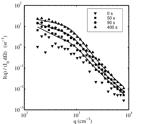
FIG. 1.: Normalized scattered intensity plotted vs. scattered wavevector $q$ at different times. The initial dataset ($\bigtriangledown$) is the intensity scattered by the initial equilibrium interface. Time is measured from the start of the partial remixing process. The figure shows the early stages of the remixing process, when the scattered intensity is increasing with time. The solid lines represent the best fit of the experimental data with Eqs. (1-3).

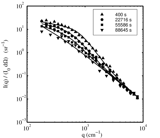
FIG. 2.: Normalized scattered intensity plotted vs. scattered wavevector $q$ after the onset the remixing process. The scattered intensity is decreasing with time. The least intense scattering ($\bigtriangledown$) is due to the final equilibrium interface. The solid lines represent the best fit of the experimental data with Eqs. (1-3).

Results for $\Delta c_{int}$ are presented in Fig. 3(a) as a function of time.

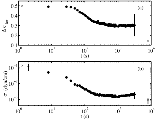
FIG. 3.: Time evolution of the concentration difference across the interface, (a), and of the interfacial surface tension, (b). Circles represent the experimental results obtained by fitting the scattered intensity distributions with Eqs. (1-3). Crosses mark the reference equilibrium values in the initial and final states. The triangle in panel (b) corresponds to the surface tension measured in the initial equilibrium state. Vertical bars on the experimental results represent the estimated fitting and sistematic errors.

Initially $\Delta c_{int}$ has its equilibrium value $\Delta c_{int}=0.5$. After about 40 seconds from the temperature increase it begins to drop, and decreases for about 300s, finally stabilizing to the constant value $\Delta c_{int}=0.3$. This is roughly a factor of two larger than the reference equilibrium value [14]. This discrepancy is due to the difficulty (both theoretical and in the fitting procedure) of clearly ascribing the measured scattered intensity to either interface or bulk phases, and an estimate of our rather large fitting and systematic error is shown with the error bars in Fig. 3. This error is such that our data cannot be considered fully quantitative, but it does not affect the features we discuss.
By combining the results for $\Delta c_{int}$ and $q_{cap}$, since from Eq.  (4)

$$\sigma\,=\,\frac{\rho\beta\Delta c_{int}g}{q_{cap}^{2}},$$ (7)

we are in the unique position to obtain the time evolution of the interfacial surface tension during the nonequilibrium process. Experimental results for the surface tension are shown in Fig. 3(b), which represents the main accomplishment of this work. The two crosses mark the value of the equilibrium surface tension at the initial and final temperature, extrapolated from the reference data from Atack and Rice [14]. The first data point represents the equilibrium surface tension measured with our light scattering setup. The agreement with the reference value is good. After the diffusion process is started the surface tension drops about two orders of magnitude, until after about 300s it stabilizes to a constant value. The asymptotic value of the surface tension is about a factor of two larger than the reference value, a good result considering the wide range of values spanned. Although these results are only partially quantitative, Fig. 3 unambiguously shows for the first time that the properties of the nonequilibrium interface rapidly attain their equilibrium values. This equilibration time is very small compared with the one associated to readjustments of the bulk phases (which corresponds to about one day), and it is comparable to the time needed to increase the temperature of the sample. Notice that the surface tension evolution does not show the initial delay seen on the $\Delta c_{int}$ evolution. This indicates that the surface tension is probably following the local temperature almost instantly, whereas $\Delta c_{int}$ does not change until diffusion has occurred over the fluctuations’ characteristic lenghtscales. With the diffusion coefficient given above this time is about 30s for the smallest wavevectors observed.

We are now in the position to comment the fast growth, shown in Fig. 1, of the scattered intensity distributions at intermediate and large wavevectors. Soon after the diffusion process is started the concentration difference across the interface decreases at its equilibrium value. According to the concentration conservation Eq. (6), a strong concentration difference $\Delta c_{bulk}$ is rapidly created in the bulk phases, and a large concentration gradient quickly grows near the interface. This gives rise to velocity-induced concentration fluctuations described by Eq. (3) [15, 16]. The growth of $\Delta c_{bulk}(t)$ during the free diffusive regime is shown by the circles in Fig. 4, and it mirrors the results for $\Delta c_{int}$ in Fig. 3(a). When enough time has passed for diffusing particles to reach the macroscopic boundaries (about 5000s as from Fig. 4), the sample enters the restricted diffusion regime, where the total concentration difference across the sample begins to change, and Eq. (6) does not hold any more. However, according to Fig. 3, we can now assume that the interfacial parameters have attained their asymptotic values. In this way we can fit the scattered intensity distributions to determine the concentration difference across the bulk phases. Results for $\Delta c_{bulk}$ obtained in this way are shown by the squares in Fig. 4.

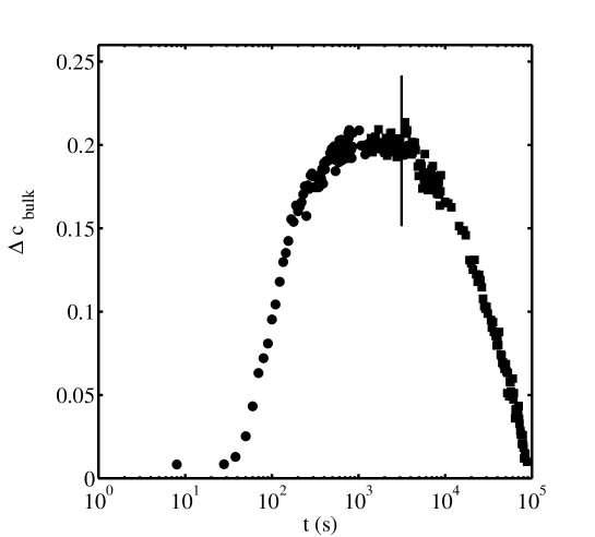
FIG. 4.: Time evolution of the concentration difference across the bulk phases. During the initial free-diffusion stage (circles) the total concentration across the sample is conserved (see Eq. (6)) and the data mirror those presented in Fig. 3(a) for the concentration difference across the interface. Later on the presence of boundaries is felt, and the sample enters the restricted-diffusion stage (squares). In agreement with the results presented in Fig. 3, we have assumed that during this stage the interfacial properties have already attained their equilibrium values.

The evolution of this process is very similar to that already observed during the free diffusion of completely miscible phases [15, 17]. From the fitting of the nonequilibrium bulk data we also determine the rolloff wavevector $q_{ro}$, which corresponds to the bump observed in the light scattering data in Figures 1-2. As outlined above and thoroughly described in Ref.[16], fluctuations at wavevectors smaller than $q_{ro}$ are stabilized by gravity, which frustrates the $q^{-4}$ divergence at small wavevectors. The rolloff wavevector is plotted in Fig. 5 as a function of time.

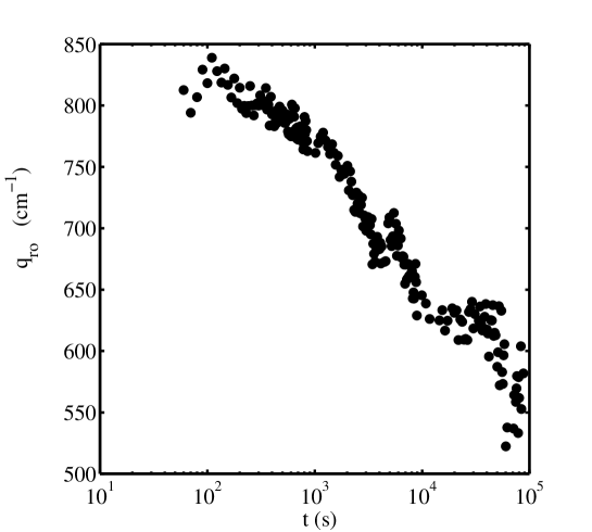
FIG. 5.: Time evolution of the rolloff wavevector $q_{ro}$.

The results displayed in Fig. 5 show that the variation of $q_{ro}$ roughly corresponds to a factor of 1.4. $q_{ro}$ is mostly determined by the layers of fluid where the concentration gradient is largest [15], that is the bulk layers close to the interface. From Eq. (5), we can estimate that the variation of the concentration gradient close to the interface is rather small, roughly corresponding to a factor four. This behavior suggests that the bulk concentration gradient is pinned to the interface concentration profile.

IV Conclusions

We have reported light-scattering measurements of the correlation function of fluctuations at the interface and in the bulk phases of a critical binary mixture undergoing diffusive partial remixing. From the intensity distributions it is clear that even during remixing a sharp interface separates the two bulk phases, and that this interface is roughened by capillary waves similar to those at equilibrium. Our data have been analyzed, yielding qualitative information on the concentration profile of the system. In particular our main results are the time evolution of the interface concentration difference and the surface tension, showing how these parameters relax to the final equilibrium values quickly compared to the system’s macroscopic equilibration time.

In this appendix we shall outline how one may derive the structure factor of fluctuations in an out of equilibrium binary mixture where a concentration gradient and a diffusive concentration flux are present. We consider a fluid described by a $z$ dependent concentration gradient $c(z)$. Layer by layer, surfaces of uniform concentration can be defined. From a macroscopic point of view these surfaces are horizontal planes. In the presence of fluctuations the surfaces are corrugated, due to the motion of parcels of fluid in the vertical direction. As customary, we will indicate by $h_{z}(x,y,t)$ the vertical displacement of the surfaces from their mean position at $z$.
In such a system light scattered with scattering vector q is proportional to the mean square amplitude of the roughness mode q, $\langle\left|h_{{\bf q}}(t)\right|^{2}\rangle$. We shall show how this quantity may be calculated for the two limiting cases of a sharp interface and a linear concentration gradient, extending the fluctuating hydrodynamics treatment applied in [16].
Throughout this paper we are dealing with small fluid velocities and overdamped motion, and equations will be approximated accordingly, see for example the discussion in [10]. We will consider the scattering of light by long-wavelength fluctuations, which scatter light mostly at small scattering angles in the forward direction.
We shall suppose fluctuations to be generated independently at different heights, and shall first consider a single fluctuation generated in a layer $dz$ at $\bar{z}$. Then, for every wavevector q, one has that $h_{z}({\bf q})$ will be maximum for $z=\bar{z}$ where the fluctuation was generated, and exponentially decreasing with distance from $\bar{z}$ like $h_{z}=h_{\bar{z}}\exp(-q|z-\bar{z}|)$. This is a consequence of the hydrodynamic equations for a viscous fluid in the case of overdamped motion [10].
The hydrodynamic equations describing motion in an incompressible viscous mixture can be linearized for small velocities [16] as:

$$div\,{\bf v}\,=\,0$$ (8)

$$\frac{\partial\,{\bf v}(x,y,z,t)}{\partial\,t}\,=\,\nu\,\nabla^{2}\,{\bf v}\,-\,\frac{1}{\rho}\,\nabla\,P(x,y,z,t)$$ (9)

$$\frac{\partial\,c}{\partial\,t}\,=\,-{\bf v}\cdot\langle\nabla c\rangle_{t}\,-\frac{1}{\rho}\,\nabla\cdot{\bf j}$$ (10)

where ${\bf v}$ is the fluctuating velocity, $c$ the fluctuating concentration, $\nu$ is the kinematic viscosity, ${P}(x,y,z,t)$ is the pressure, $\langle\nabla c\rangle_{t}$ is the concentration gradient averaged over typical fluctuations’ timescales and ${\bf j}$ is the mass diffusion flux. Equation (8) is the usual mass conservation equation for an incompressible fluid, Eq. (9) is the linearized Navier–Stokes equation, and Eq. (10) is the convection-diffusion equation. The macroscopic diffusive flux ${\bf j}$ is proportional to $\nabla\mu$, where $\mu$ is the chemical potential of the mixture; it is non–zero where $\mu$ is not constant.
Equiconcentration surfaces are corrugated by thermal velocity fluctuations in the vertical direction, and these are described by the $z$ component of Eq. (9).
We change variable from $c$ to $h$ in Eq. (10), and simplify the equation by assuming that concentration diffusion obeys Fick’s law $\frac{\partial h}{\partial t}=D\nabla^{2}h$, where $D$ is the ”mutual diffusion” coefficient.
From Eq. (10) we take the $z$ component of the velocity, $v_{z}\,=\,\frac{\partial}{\partial\,t}h\,+\,D\nabla^{2}h$, and substitute it into equation (9), obtaining, after Fourier transform in $x,y$ and $t$, an equation of motion for non-equilibrium fluctuations:

$$-i\,\omega\,\left[\,-i\,\omega\,h_{{\bf q},\omega}(z)\,+\,2D\,q^{2}\,h_{{\bf q},\omega}(z)\,\right]\, =$$ (11)

$$=\,2\,\nu\,q^{2}\,\left[\,-i\,\omega\,h_{{\bf q},\omega}(z)\,+\,2D\,q^{2}\,h_{{\bf q},\omega}(z)\,\right]\,-\,\frac{1}{\rho}\,q\,P_{{\bf q},\omega}(z)\, + \,\frac{1}{\rho}\,q\,S_{{\bf q},\omega},$$ (12)

where the continuity of tangential stresses on the fluctuating surface has been imposed and a stocastic force term $S_{\bf q}$ has been added to describe the onset of thermal spontaneous velocity fluctuations. The correlation function of this stocastic force is assumed to be (see [18]) $\langle\left|\frac{1}{\rho}{q}{S}_{{\bf q}\,\omega}\right|^{2}\rangle\,=\,k_{B}T\frac{2\,\nu\,q^{3}}{\rho\,A}$ as in equilibrium.
The pressure P in Eq. (LABEL:motointerfacciah2diff) may be exerted by the external gravity force and by internal capillary forces and is measured against the average fluid pressure. Because of Eqs. (8)-(9), in deriving Eq. (LABEL:motointerfacciah2diff) we have imposed that the pressure $P(\bar{z})$ induced by the fluctuation in layer $\bar{z}$ decays exponentially with distance from the fluctuation layer to the average pressure, like $P_{\bf q}(z)\,=\,P_{\bf q}(\bar{z})\,\exp\left({-\,q\,|z-\bar{z}|}\right)$. This pressure term depends on the local concentration profile. It can be written explicitly for fluctuations involving a ”sharp interface” profile and for those in the bulk phases, by considering the gravity and capillary forces on the fluctuations. We shall consider a fluctuation to be a sharp-interface fluctuation if $\bar{z}$ is close to the interface position $z_{i}$. Instead, if $\partial_{z}c(z)$ may be considered linear within a range of $\pm\frac{1}{q}$ around $\bar{z}$, the fluctuation will be considered a bulk fluctuation. Our treatment is approximate in that we are supposing that every fluctuation falls within one of these cases.
Interface fluctuations and bulk fluctuations give rise to different dynamics.
In the case of a sharp interface, the pressure acting on a fluid element at height $\bar{z}=z_{i}$, when a fluctuation occurs at $z_{i}$ bending the interface, is:

$$P_{\bf q}(z_{i})\,=\,\frac{1}{2}\,\left[\,\Delta\rho\,g\,h_{\bf q}(z_{i})\,+\,\sigma\,q^{2}\,h_{\bf q}(z_{i})\right].$$ (14)

Substituting this pressure in Eq. (LABEL:motointerfacciah2diff) one may, with algebra similar to that in [16], calculate the spectrum of interface fluctuations:

$$\left|h_{{\bf q}\,\omega}\right|^{2}\,=\,{\langle\left|h({\bf q})\right|^{2}\rangle}_{t}\,\frac{2\frac{\Delta\rho\,g\,q\,+\,\sigma\,q^{3}\,+\,4\,\rho\,\nu\,D\,q^{4}}{4\,\rho\,\nu\,q^{2}}}{\omega^{2}\,+\,\left(\frac{\Delta\rho\,g\,q\,+\,\sigma\,q^{3}\,+\,4\,\rho\,\nu\,D\,q^{4}}{4\,\rho\,\nu\,q^{2}}\right)^{2}},$$ (15)

where the static term is:

$${\langle\left|h({\bf q})\right|^{2}\rangle}_{t}\,=\,\frac{1}{A}\frac{k_{B}T}{\Delta\rho\,g\,+\,\sigma\,q^{2}\,+\,4\,\rho\,\nu\,D\,q^{3}}.$$ (16)

At equilibrium, when the mutual diffusion coefficient $D\,=\,0$, the spectrum linewidth is the same as that of the well-known equilibrium interface [5, 10]: gravity dominates at small wavevectors and capillary forces at large ones. However, during the nonequilibrium process, diffusion is effective in relaxing large–wavevector fluctuations. At these wavevectors the linewidth becomes the usual diffusive $Dq^{2}$ one, and this diffusive contribution is also apparent in the static structure factor where a new term proportional to $q^{3}$ is present in the denominator. With our setup it was not possible to study the structure factor at large enough wavevectors to check the result and, as far as we know, this feature has never been observed.
The other case is that of a bulk phase where the concentration gradient is approximately linear. Here the pressure opposing a fluid element at height $\bar{z}$ when a fluctuation occurs bending the layer at height $\bar{z}$ is:

$$P_{\bf q}(\bar{z})\,=\,\frac{1}{2}\,\left[\,\partial_{z}\rho\,g\,h_{\bf q}(\bar{z})\,+\,\partial_{z}\sigma\,q^{2}\,h_{\bf q}(\bar{z})\right]\,\frac{2}{q},$$ (17)

where $\partial_{z}$ stands for $\frac{\partial}{\partial\,z}$.
From mean field theories of binary systems [19, 20] it follows that $\frac{\partial\,\sigma}{\partial\,z}\,\propto\,\left(\frac{\partial\,\rho}{\partial\,z}\right)^{2}$. If the concentration gradient is small, the capillary term becomes negligible compared to the gravitational one, and we shall drop it from now on in this case. As before, from Eq. (LABEL:motointerfacciah2diff) one may calculate the correlation function of bulk fluctuations, recovering the spectrum calculated and commented in Ref. [16]:

$$\left|h_{{\bf q}\,\omega}(z)\right|^{2}\,=\,{\langle\left|h({\bf q},z)\right|^{2}\rangle}_{t}\,\frac{2\,\frac{2\,\partial_{z}\rho\,g\,+\,4\,\rho\,\nu\,D\,q^{4}}{4\,\rho\,\nu\,q^{2}}}{\omega^{2}\,+\,\left(\frac{2\,\partial_{z}\rho\,g\,+\,4\,\rho\,\nu\,D\,q^{4}}{4\,\rho\,\nu\,q^{2}}\right)^{2}},$$ (18)

where the static term is

$${\langle\left|h({\bf q},z_{i})\right|^{2}\rangle}_{t}\,=\,\frac{1}{A\,{\frac{2}{q}}}\,\frac{k_{B}T}{\partial_{z}\rho\,g\,+\,2\rho\,\nu\,D\,q^{4}}.$$ (19)

Although these bulk fluctuations have the same origin as capillary waves, namely velocity fluctuations parallel to the concentration gradient, the transition from a sharp to a diffuse interface radically modifies both the static and the dynamic structure factor of the fluctuations.
We shall now outline how one may evaluate the intensity of light scattered by these fluctuations. Suppose a plane wave having wavevector $K_{0}$ in vacuum and intensity $I_{0}$ is propagating in the vertical direction in a sample having index of refraction $n=n(z)$. The roughness of the equiconcentration surfaces due to a fluctuation at $\bar{z}$ introduces a phase dependancy on $(x,y)$. One easily sees that the resulting scattered intensity per solid angle is $\frac{dI_{{\bf q},t}}{d\Omega\,}\,=\,I_{0}\,\frac{n^{2}\,K_{0}^{4}}{(2\pi)^{2}}\,\left|\Delta\Phi({\bf q},t)\right|^{2}$, where $\Delta\Phi({\bf q},t)$ is the optical path variation induced by the fluctuation given by

$$\Delta\Phi({\bf q},t)\,=\,\frac{\partial n}{\partial c}\,\int dz\,h_{z}({\bf q},t)\,\,\partial_{z}c(z).$$ (20)

This integral is similar to that required to calculate the pressures of Eqs. (14) and (17) and, depending on the system’s local concentration profile at $\bar{z}$, it can be easily approximated in the same two limiting cases considered above, sharp interface or concentration gradient in bulk phase.

Scattering from the whole sample is given by integration over the sample thickness of the scattering due to fluctuations arising in a single layer, weighed with the probability of being in that layer and with the density of fluctuations, so that one integrates the single fluctuation intensity in $d\bar{z}\frac{q}{2}$.
If the sample comprises both bulk regions and a sharp interface having a concentration difference $\Delta c_{int}$, the total scattered light is then:

$$\frac{dI_{{\bf q},t}}{d\Omega\,}\,=\,I_{0}\,\frac{n^{2}\,K_{0}^{4}}{(2\pi)^{2}}\,\left(\frac{\partial n}{\partial c}\right)^{2}\,\left[\left(\Delta c_{int}\right)^{2}\,\left|h_{z_{i}}({\bf q},t)\right|^{2}\,+\,\int_{bulk}d\bar{z}\frac{2}{q}\left[\partial_{z}c(z)\Bigg{|}_{\bar{z}}\right]^{2}\left|h_{\bar{z}}({\bf q},t)\right|^{2}\right]$$ (21)

(22)

We have used Eq. (22) to fit our data after approximating the bulk phase integral by considering that most of the scattering is due to the layers with the greatest $\partial_{z}c(z)$.

REFERENCES

- [1] L.I.Mandelstam, Ann. der Physik 41, 609 (1913).
- [2] R.H.Katyl,and U.Ingard, Phys. Rev. Lett. 20, 248 (1968).
- [3] J.S.Huang, and W.W.Webb, Phys. Rev. Lett. 23, 160 (1969).
- [4] J.Zollweg, G.Hawkins, and G.B.Benedek, Phys. Rev. Lett. 27, 1182 (1971).
- [5] M.A.Bouchiat, and J.Meunier, J. de Physique Colloque 33, C1-141 (1972).
- [6] D.D. Joseph,Eur. J. Mech., B/Fluids 9, 565 (1990).
- [7] S.E.May, and J.V.Maher, Phys. Rev. Lett. 67, 2013 (1991).
- [8] P. Petitjeans, C. R. Acad. Sci. Paris 322, 673 (1996).
- [9] D.H.Vlad, and J.V.Maher, Phys. Rev. E 59, 476 (1999).
- [10] D.Langevin, Light scattering by liquid surfaces and complementary techniques. (Dekker, New York, 1992).
- [11] M.A.Bouchiat, and J.Meunier, J. de Physique 32, 5611 (1971).
- [12] M.Carpineti et al., Phys. Rev. A 42, 7347 (1990).
- [13] A.Vailati, and M.Giglio, Phys. Rev. Lett. 77, 1484 (1996).
- [14] D.Atack, and O.K.Rice, Discuss. Faraday Soc. 15, 210 (1953).
- [15] A.Vailati, and M.Giglio, Nature 390, 262 (1997).
- [16] A.Vailati, and M.Giglio, Phys. Rev. E 58, 4361 (1998).
- [17] D.Brogioli, A.Vailati, and M.Giglio, Phys. Rev. E 61, R1 (2000).
- [18] C.Cohen, J.W.H.Sutherland, and J.M.Deutch, Phys. Chem. Liq. 2, 213 (1971).
- [19] J.W.Cahn, and J.E.Hilliard, J. Chem. Phys. 28, 258 (1958).
- [20] S.A.Safran, Statistical thermodynamics of surfaces, interfaces and membranes. (Addison-Wesley, Reading, 1994).