Many-body CPA for the Holstein-DE model

Abstract

A many-body coherent potential approximation (CPA) previously developed for the double exchange (DE) model is extended to include coupling to local quantum phonons. The Holstein-DE model studied (equal to the Holstein model for zero Hund coupling) is considered to be a simple model for the colossal magnetoresistance manganites. We concentrate on effects due to the quantisation of the phonons, such as the formation of polaron subbands. The electronic spectrum and resistivity are investigated for a range of temperature and electron-phonon coupling strengths. Good agreement with experiment is found for the Curie temperature and resistivity with intermediate electron-phonon coupling strength, but phonon quantisation is found not to have a significant effect in this coupling regime.

I Introduction

In this paper we study the Holstein-DE (double exchange) model

$$\ H=\sum_{ij\sigma}t_{ij}^{\mbox{ }}c^{{\dagger}}_{i\sigma}c_{j\sigma}^{\mbox{ }}-J\sum_{i}{\bf{S}}_{i}^{\mbox{ }}\cdot\vec{\sigma}_{i}^{\mbox{ }}-h\sum_{i}L^{z}_{i}-g\sum_{i}n_{i}^{\mbox{ }}\left(b^{{\dagger}}_{i}+b_{i}^{\mbox{ }}\right)+\omega\sum_{i}n^{b}_{i}$$ (1)

where $i$ and $j$ are site indices, $c^{{\dagger}}_{i\sigma}$ and $b^{{\dagger}}_{i}$ ($c_{i\sigma}^{\mbox{ }}$ and $b_{i}^{\mbox{ }}$) create (annihilate) an electron of spin $\sigma$ and a phonon respectively, ${\bf{S}}_{i}$ is a local spin, $\vec{\sigma}_{i}=(1/2)\sum_{\sigma\sigma^{\prime}}c^{{\dagger}}_{i\sigma}\vec{\sigma}_{\sigma\sigma^{\prime}}^{\mbox{ }}c_{i\sigma^{\prime}}^{\mbox{ }}$ is the electron spin operator ($\vec{\sigma}_{\sigma\sigma^{\prime}}$ being the Pauli matrix), $L^{z}_{i}=S^{z}_{i}+\sigma^{z}_{i}$ is the $z$-component of angular momentum, $n_{i}^{\mbox{ }}=\sum_{\sigma}c^{{\dagger}}_{i\sigma}c_{i\sigma}^{\mbox{ }}$ and $n^{b}_{i}=b^{{\dagger}}_{i}b_{i}^{\mbox{ }}$. The parameter $t_{ij}$ is the hopping integral, $J>0$ is the Hund coupling, $h$ is the Zeeman energy, $g$ is the electron-phonon coupling strength and $\omega$ is the Einstein phonon energy. $H$ is a model for the colossal magnetoresistance (CMR) manganite compounds with the double degeneracy of the conduction band neglected and a simplified form assumed for the electron-phonon coupling and phonon dispersion. The electron-phonon coupling in Eq. (1) is of the breathing-mode form, i.e. $-g^{\prime}\sum_{i}n_{i}x_{i}$ in the classical limit (where $x_{i}$ is the phonon displacement), but we regard it as an effective Jahn-Teller coupling.

Hamiltonian (1) was first studied by Röder et al [2], who treated the Hund coupling using a mean-field approximation and the electron-phonon coupling using a variational Lang-Firsov approximation. The same authors later used a similar method to study a more realistic model for CMR systems [3]. In this paper we treat both the Hund and the electron-phonon coupling using an extension of a many-body coherent potential approximation (CPA) previously derived for the DE model [4, 5]. The CPA treats the Hund coupling better than mean-field theory and has the advantage over Lang-Firsov variational methods that the whole of the electronic spectrum can be studied, not just the coherent polaron band near the Fermi energy. In the limit of classical spins and phonons Millis et al used dynamical mean-field theory (DMFT) to study another more realistic model for CMR materials [6, 7]. Here however we concentrate on the effects of quantisation of the phonons.

Our approach has many similarities with studies of the Holstein model using DMFT, which have been carried out for the classical phonon [8] and empty-band [9] limits in which the model is a one-electron problem. Indeed the standard dynamical CPA is equivalent to DMFT for one-electron problems such as the binary alloy [10], the DE and Holstein models in the empty-band limit [9, 11, 12], and the DE model with classical local spins [5]. DMFT should be regarded as the correct extension of the CPA to many-body problems [13]. For the current many-body problem we regard our CPA as an approximate solution of DMFT, or as an extrapolation from the one-electron case. The CPA has the advantage of relative analytic simplicity, but does not treat the many-body dynamics as well as DMFT, retaining too much one-electron character.

The many-body CPA derived for the finite $S$ DE model in Ref. [4] and Ref. [5] was based on Hubbard’s scattering correction approximation for the Hubbard model [14]. Hubbard’s approximation was derived by decoupling Green function equations of motion (EOM) according to an alloy analogy in which electrons of one spin are frozen while the propagation of those of the opposite spin is considered (within the CPA). Although more modern formulations of the CPA exist Hubbard’s EOM approach was found to be particularly suitable for extension to the DE model, where the possibility of electrons exchanging (spin) angular momentum with local spins complicates the problem. The resulting many-body CPA was exact in the atomic limit $t_{ij}\rightarrow 0$ and recovered the one-electron CPA/DMFT in the empty-band and classical spin ($S\rightarrow\infty$) limits.

In Sec. II we solve the atomic limit of Hamiltonian (1), and in Sec. III we extend our many-body CPA to the Holstein-DE model. The properties of the CPA solution are discussed in Sec. IV, and the special case ($J=h=0$) of the Holstein model is considered in Sec.  V. We give a summary in Sec.  VI.

II The atomic limit

In the atomic limit $t_{ij}\rightarrow 0$ $H$ is exactly solvable using the canonical transformation $H\mapsto\tilde{H}=e^{\nu^{{\dagger}}}He^{\nu}$ where $\nu=\frac{g}{\omega}n(b^{{\dagger}}-b)$ (Ref. [15]) (we drop site indices). In the presence of electron-phonon coupling the phonon potential is of the displaced harmonic oscillator form, and the effect of the canonical transformation is to shift the operators to take account of this: $b\mapsto b+\frac{g}{\omega}n$ and $c_{\sigma}^{\mbox{ }}\mapsto Xc_{\sigma}^{\mbox{ }}$ where $X=\exp(g/\omega(b^{{\dagger}}-b))$. This transformation decouples the Hamiltonian $\tilde{H}=H_{b}+H_{f}$ into a bosonic component $H_{b}=\omega n^{b}$ and a fermionic component $H_{f}=-J{\bf{S}}\cdot\vec{\sigma}-hL^{z}-g^{2}/\omega\,n^{2}$ where $g^{2}/\omega=:\lambda\omega$ is the binding energy of a polaron.

The one-electron Green function $G_{\sigma}(t)=-i\theta(t)\langle\{c_{\sigma}(t),c_{\sigma}^{{\dagger}}\}\rangle$ can be separated into fermionic and bosonic traces using the invariance of the trace under cyclic permutations and $e^{\nu^{{\dagger}}}e^{\nu}=1$,

$$G_{\sigma}(t)=-i\theta(t)\left[\frac{{\rm Tr}_{f}\{e^{-\beta H_{f}}e^{iH_{f}t}c_{\sigma}e^{-iH_{f}t}c^{{\dagger}}_{\sigma}\}}{{\rm Tr}_{f}\{e^{-\beta H_{f}}\}}\frac{{\rm Tr}_{b}\{e^{-\beta H_{b}}e^{iH_{b}t}Xe^{-iH_{b}t}X^{{\dagger}}\}}{{\rm Tr}_{b}\{e^{-\beta H_{b}}\}}\right.$$ (2)

$$\nopagebreak\left.+\frac{{\rm Tr}_{f}\{e^{-\beta H_{f}}c^{{\dagger}}_{\sigma}e^{iH_{f}t}c_{\sigma}e^{-iH_{f}t}\}}{{\rm Tr}_{f}\{e^{-\beta H_{f}}\}}\frac{{\rm Tr}_{b}\{e^{-\beta H_{b}}X^{{\dagger}}e^{iH_{b}t}Xe^{-iH_{b}t}\}}{{\rm Tr}_{b}\{e^{-\beta H_{b}}\}}\right].$$ (3)

We evaluate the bosonic traces directly and the fermionic traces using the equation of motion (EOM) method, and in the energy representation $G_{\sigma}(\epsilon)=\int_{-\infty}^{\infty}{\rm d}t\,e^{i\epsilon t}G_{\sigma}(t)$ obtain

$$G_{\sigma}(\epsilon)=\sum_{r=-\infty}^{\infty}\frac{{\rm I}_{r}\left(2\lambda\sqrt{b(\omega)(b(\omega)+1)}\,\right)}{(2S+1)\exp(\lambda(2b(\omega)+1))}\sum_{\alpha=\pm}\left[\frac{e^{r\beta\omega/2}\,W^{0+}_{\alpha\sigma}+e^{-r\beta\omega/2}\,W^{0-}_{\alpha\sigma}}{\epsilon-\alpha JS/2+h\sigma/2+\lambda\omega(1+2\delta_{\alpha+})+\omega r}\right.$$ (4)

$$\left.+\frac{e^{r\beta\omega/2}\,W^{1+}_{\alpha\sigma}+e^{-r\beta\omega/2}\,W^{1-}_{\alpha\sigma}}{\epsilon+\alpha J/2(S+1)+h\sigma/2+\lambda\omega(1+2\delta_{\alpha+})+\omega r}\right].$$ (5)

Here the weight factors

$$W^{0\gamma}_{\alpha\sigma}=(S+1)\left\langle n^{\alpha}_{-\sigma}n^{\gamma}_{\sigma}\right\rangle-\alpha\sigma\left\langle S^{z}n^{\alpha}_{-\sigma}n^{\gamma}_{\sigma}\right\rangle+\left(1-\delta_{\alpha\gamma}\right)\left\langle S^{-\sigma}\sigma^{+\sigma}\right\rangle$$ (7)

$$W^{1\gamma}_{\alpha\sigma}=S\left\langle n^{\alpha}_{-\sigma}n^{\gamma}_{\sigma}\right\rangle+\alpha\sigma\left\langle S^{z}n^{\alpha}_{-\sigma}n^{\gamma}_{\sigma}\right\rangle-\left(1-\delta_{\alpha\gamma}\right)\left\langle S^{-\sigma}\sigma^{+\sigma}\right\rangle,$$ (8)

$\alpha$, $\gamma=\pm$, $\delta_{\alpha+}=1$ for $\alpha=+$ and $0$ for $\alpha=-$, ${\rm I}_{r}$ is the modified Bessel function, $b(\omega)=1/(\exp(\beta\omega)-1)$ is the Bose function, and we define $n^{+}_{\sigma}=n_{\sigma}$, $n^{-}_{\sigma}=1-n_{\sigma}$, and $S^{-\sigma}\sigma^{+\sigma}=S^{-}\sigma^{+}$ for $\sigma=\uparrow$ and $S^{+}\sigma^{-}$ for $\sigma=\downarrow$.

In the ($J=h=0$) case of the Holstein model Eq. (5) reduces to the formula

$$G_{\sigma}(\epsilon)=\sum_{r=-\infty}^{\infty}\frac{{\rm I}_{r}\left(2\lambda\sqrt{b(\omega)(b(\omega)+1)}\,\right)}{\exp(\lambda(2b(\omega)+1))}\left[\frac{e^{r\beta\omega/2}\langle n^{-}_{-\sigma}n_{\sigma}\rangle+e^{-r\beta\omega/2}\langle n^{-}_{-\sigma}n^{-}_{\sigma}\rangle}{\epsilon+\lambda\omega+\omega r}\right.$$ (9)

$$\left.+\frac{e^{r\beta\omega/2}\langle n_{-\sigma}n_{\sigma}\rangle+e^{-r\beta\omega/2}\langle n_{-\sigma}n^{-}_{\sigma}\rangle}{\epsilon+3\lambda\omega+\omega r}\right],$$ (10)

but we are mostly interested in the strong Hund-coupling limit, so we shift the energy to have the zero near the Fermi level, $\epsilon\mapsto\epsilon-JS/2$, and let $J\rightarrow\infty$. In this limit we find

$$G_{\sigma}(\epsilon)=\sum_{r=-\infty}^{\infty}\frac{{\rm I}_{r}\left(2\lambda\sqrt{b(\omega)(b(\omega)+1)}\,\right)}{(2S+1)\exp(\lambda(2b(\omega)+1))}\frac{e^{r\beta\omega/2}\,W^{+}_{\sigma}+e^{-r\beta\omega/2}\,W^{-}_{\sigma}}{\epsilon+h\sigma/2+\omega r+\lambda\omega}$$ (11)

where the weight factors

$$W^{+}_{\sigma}= \left\langle(S+1+\sigma S^{z})n_{\sigma}+S^{-\sigma}\sigma^{+\sigma}\right\rangle =(2S+1)\left(\frac{n}{2}+\sigma\left\langle\sigma^{z}\right\rangle\right)$$ (13)

$$W^{-}_{\sigma}= \left\langle(1-n)(S+1+\sigma S^{z})\right\rangle =(S+1)(1-n)+\sigma\left\langle S^{z}\right\rangle-2S\sigma\left\langle\sigma^{z}\right\rangle.$$ (14)

The paramagnetic state spectrum of Eq. (11) is plotted in Fig. 1 for the classical spin limit $S\rightarrow\infty$ at quarter-filling $n=0.5$. The spectrum consists of delta-function peaks separated in energy by $\omega$, and for clarity we include the peaks’ envelope curve in Fig.  1. Note that the symmetry of the spectrum about zero energy is due to choice of filling $n=0.5$; in general the lower and upper (zero temperature) ‘bands’ have weights $n$ and $1-n$ respectively. By counting weights it may be seen that for any $n$ the zero temperature chemical potential $\mu(T=0)=0$ lies in the zero energy peak in the middle of the pseudogap.

III The CPA Green function

We now derive a many-body CPA for the one-electron Green function $G^{ij}_{\sigma}(\epsilon)$ of the full Hamiltonian (1). As discussed in the introduction we proceed by decoupling equations of motion (EOM), adapting decoupling approximations previously used for the DE model [5]. Recall that with the fermionic definition of Green functions, $\langle\langle A\,;C\rangle\rangle_{\epsilon}=-i\int_{0}^{\infty}{\rm d}t\,\exp(i\epsilon t)\langle\{A(t),C\}\rangle$, the EOM is

$$\epsilon\,\left\langle\left\langle A\,;C\right\rangle\right\rangle_{\epsilon}=\left\langle\{A,C\}\right\rangle+\left\langle\left\langle[A,H]\,;C\right\rangle\right\rangle_{\epsilon}.$$ (15)

As in Ref. [5] and in the original version of this method due to Hubbard [14] we split the Green function into a low-energy component $G^{ij-}_{\sigma}(\epsilon)=\langle\langle n^{-}_{i}c_{i\sigma}^{\mbox{ }};c^{{\dagger}}_{j\sigma}\rangle\rangle_{\epsilon}$ and a high-energy component $G^{ij+}_{\sigma}(\epsilon)=\langle\langle n^{+}_{i}c_{i\sigma}^{\mbox{ }};c^{{\dagger}}_{j\sigma}\rangle\rangle_{\epsilon}$, i.e. $G^{ij}_{\sigma}(\epsilon)=\sum_{\alpha=\pm}G^{ij\alpha}_{\sigma}(\epsilon)$. To close the system of EOM we in fact need to introduce the Green functions

$$S^{ij\alpha}_{\sigma}(\vec{r},\epsilon) = \left\langle\left\langle\Gamma_{i}(\vec{r})n^{\alpha}_{i}c_{i\sigma}^{\mbox{ }};c^{{\dagger}}_{j\sigma}\right\rangle\right\rangle_{\epsilon}$$ (17)

$$T^{ij\alpha}_{\sigma}(\vec{r},\epsilon) = \left\langle\left\langle\Gamma_{i}(\vec{r})n^{\alpha}_{i}S^{-\sigma}_{i}c_{i-\sigma}^{\mbox{ }};c^{{\dagger}}_{j\sigma}\right\rangle\right\rangle_{\epsilon}$$ (18)

where $\vec{r}=(\rho,\phi,\theta)$ is a parameter and the operator $\Gamma_{i}(\vec{r})=\exp(\rho S^{z}_{i})\exp(\phi b^{{\dagger}}_{i})\exp(\theta b_{i})$. Note that $\Gamma$ is a generating function for the operators $S^{z}$, $b^{{\dagger}}$ and $b$, so that $\partial^{n}/\partial\phi^{n}\Gamma_{i}(\vec{r})=(b^{{\dagger}}_{i})^{n}\Gamma_{i}(\vec{r})$ for instance. This is convenient in allowing us to close the system of EOM with a minimal number of equations.

When writing the EOM we use the convenient commutation identities $[e^{\phi b^{{\dagger}}},b]=-\phi e^{\phi b^{{\dagger}}}$ and $[e^{\theta b},b^{{\dagger}}]=\theta e^{\theta b}$, and the Feynman operator disentanglement relation $e^{A+B}=e^{A}e^{B}e^{-1/2[A,B]}$, which holds if $[[A,B],A]=[[A,B],B]=0$. We also work for $\sigma=\uparrow$; the $\sigma=\downarrow$ equations can be obtained using the symmetry of $H$. We introduce the operator

$$K^{\alpha}(\theta,\phi)=\omega\left(\phi\frac{\partial}{\partial\phi}-\theta\frac{\partial}{\partial\theta}\right)+g\left(\frac{\partial}{\partial\phi}+\frac{\partial}{\partial\theta}+\theta+\delta_{\alpha+}(\theta-\phi)\right),$$ (19)

and obtain the (exact) EOM

$$\left[\epsilon+\frac{h}{2}+\frac{J}{2}\frac{\partial}{\partial\rho}+K^{\alpha}(\theta,\phi)\right]S^{ij\alpha}_{\uparrow}(\vec{r},\epsilon)+\frac{J}{2}e^{\rho\delta_{\alpha+}}T^{ij\alpha}_{\uparrow}(\vec{r},\epsilon)=\delta_{ij}\left\langle\Gamma(\vec{r})n^{\alpha}_{\downarrow}\right\rangle\hskip 72.26999pt$$ (20)

$$+\left\langle\left\langle\Gamma_{i}(\vec{r})\left[n^{\alpha}_{i\downarrow},H_{0}\right]c_{i\uparrow};c^{{\dagger}}_{j\uparrow}\right\rangle\right\rangle_{\epsilon}+\sum_{k}t_{ik}\left\langle\left\langle\Gamma_{i}(\vec{r})n^{\alpha}_{i\downarrow}c_{k\uparrow};c^{{\dagger}}_{j\uparrow}\right\rangle\right\rangle_{\epsilon}$$ (21)

for $S^{ij\alpha}_{\uparrow}(\vec{r},\epsilon)$ and

$$\left[\epsilon+\frac{h}{2}-\frac{J}{2}\left(\delta_{\alpha-}+\frac{\partial}{\partial\rho}\right)+K^{\alpha}(\theta,\phi)\right]T^{ij\alpha}_{\uparrow}(\vec{r},\epsilon)\hskip 180.67499pt$$ (22)

$$+\frac{J}{2}e^{-\rho\delta_{\alpha+}}\left[S(S+1)+\alpha\frac{\partial}{\partial\rho}-\frac{\partial^{2}}{\partial\rho^{2}}\right]S^{ij\alpha}_{\uparrow}(\vec{r},\epsilon)=-\alpha\delta_{ij}\left\langle\Gamma(\vec{r})S^{-}\sigma^{+}\right\rangle$$ (23)

$$+\left\langle\left\langle\Gamma_{i}(\vec{r})\left[n^{\alpha}_{i\uparrow},H_{0}\right]S^{-}_{i}c_{i\downarrow};c^{{\dagger}}_{j\uparrow}\right\rangle\right\rangle_{\epsilon}+\sum_{k}t_{ik}\left\langle\left\langle\Gamma_{i}(\vec{r})n^{\alpha}_{i\uparrow}S^{-}_{i}c_{k\downarrow};c^{{\dagger}}_{j\uparrow}\right\rangle\right\rangle_{\epsilon}$$ (24)

for $T^{ij\alpha}_{\uparrow}(\vec{r},\epsilon)$. Here $H_{0}$ is the electron hopping term of the Hamiltonian and we have dropped site indices in the expectations, assuming a homogeneous state. Equations (21) and (24) should be compared with their analogues for the DE model case: equations (4) and (5) in Ref. [5].

As usual we now neglect the penultimate Green functions in equations (21) and (24) (the ones containing $[n^{\alpha}_{i\sigma},H_{0}]$). This corresponds to making the alloy analogy. We treat the final Green functions in these equations using a CPA and treat all other terms exactly. In fact we use the approximations

$$\sum_{k}t_{ik}\left\langle\left\langle\Gamma_{i}(\vec{r})n^{\alpha}_{i\downarrow}c_{k\uparrow}^{\mbox{ }}\,;c^{{\dagger}}_{j\uparrow}\right\rangle\right\rangle_{\epsilon}\approx\left\langle\Gamma(\vec{r})n^{\alpha}_{\downarrow}\right\rangle\left(\sum_{k}t_{ik}G^{kj}_{\uparrow}(\epsilon)-J_{\uparrow}(\epsilon)G^{ij}_{\uparrow}(\epsilon)\right)+J_{\uparrow}(\epsilon)S^{ij\alpha}_{\uparrow}(\vec{r},\epsilon)$$ (26)

$$\sum_{k}t_{ik}\left\langle\left\langle\Gamma_{i}(\vec{r})n^{\alpha}_{i\uparrow}S^{-}_{i}c_{k\downarrow}^{\mbox{ }}\,;c^{{\dagger}}_{j\uparrow}\right\rangle\right\rangle_{\epsilon}\approx-\alpha\left\langle\Gamma(\vec{r})S^{-}\sigma^{+}\right\rangle\left(\sum_{k}t_{ik}G^{kj}_{\uparrow}(\epsilon)-J_{\uparrow}(\epsilon)G^{ij}_{\uparrow}(\epsilon)\right)\hskip 32.52127pt$$ (27)

$$+J_{\downarrow}(\epsilon+h)T^{ij\alpha}_{\uparrow}(\vec{r},\epsilon)$$ (28)

where $J_{\sigma}(\epsilon)=\epsilon-\Sigma_{\sigma}(\epsilon)-G_{\sigma}(\epsilon)^{-1}$, $\Sigma_{\sigma}(\epsilon)$ and $G_{\sigma}(\epsilon)$ being the self-energy and local Green function respectively. The function $E_{\sigma}(\epsilon)=\epsilon-J_{\sigma}(\epsilon)$ is related to the Weiss function of DMFT, $E_{\sigma}(i\omega_{n})\equiv{\cal G}^{-1}_{\sigma}(i\omega_{n})$, $i\omega_{n}$ being a fermionic Matsubara frequency. Equations (26) and (28) are generalisations of Hubbard’s scattering correction approximation [14], and lead to the CPA equations in the case of the DE model. We make these particular approximations since Eq. (26) and Eq. (28) are of the usual CPA form, but do not give a formal justification.

We define $E^{h}_{\sigma}(\epsilon)=E_{\sigma}(\epsilon+h\delta_{\sigma\downarrow})+\sigma h/2$ and $\lambda^{ij}_{\sigma}(\epsilon)=\delta_{ij}+\sum_{k}t_{ik}G^{kj}_{\sigma}(\epsilon)-J_{\sigma}(\epsilon)G^{ij}_{\sigma}(\epsilon)$, and from equations (21), (24), (26) and (28) obtain

$$\left[\begin{array}[]{cc}E^{h}_{\uparrow}(\epsilon)+\frac{J}{2}\frac{\partial}{\partial\rho}+K^{\alpha}(\theta,\phi)&\frac{J}{2}e^{\rho\delta_{\alpha+}}\\ \frac{J}{2}e^{-\rho\delta_{\alpha+}}\left(S(S+1)+\alpha\frac{\partial}{\partial\rho}-\frac{\partial^{2}}{\partial\rho^{2}}\right)&E^{h}_{\downarrow}(\epsilon)-\frac{J}{2}\left(\delta_{\alpha-}+\frac{\partial}{\partial\rho}\right)+K^{\alpha}(\theta,\phi)\end{array}\right]\left(\begin{array}[]{c}S^{ij\alpha}_{\uparrow}(\vec{r},\epsilon)\\ T^{ij\alpha}_{\uparrow}(\vec{r},\epsilon)\end{array}\right)$$ (33)

$$\approx\lambda^{ij}_{\uparrow}(\epsilon)\left(\begin{array}[]{c}\left\langle\Gamma(\vec{r})n^{\alpha}_{\downarrow}\right\rangle\\ -\alpha\left\langle\Gamma(\vec{r})S^{-}\sigma^{+}\right\rangle\end{array}\right).$$ (36)

We make no further approximations. We use the top row of Eq. (36) to eliminate $T^{ij\alpha}_{\uparrow}(\vec{r},\epsilon)$, obtaining a second-order linear (parabolic) PDE for $S^{ij\alpha}_{\uparrow}(\vec{r},\epsilon)$. We take $i=j$ and use $\lambda^{ii}_{\sigma}(\epsilon)=1$ (Ref. [5]). In the strong Hund-coupling limit $J\rightarrow\infty$, which we take with the energy origin shifted as $\epsilon\mapsto\epsilon-JS/2$, this second-order PDE simplifies to the first-order linear PDE

$$\left[\frac{(1+S)E^{h}_{\uparrow}(\epsilon)+SE^{h}_{\downarrow}(\epsilon)}{2S+1}+\frac{E^{h}_{\uparrow}(\epsilon)-E^{h}_{\downarrow}(\epsilon)}{2S+1}\frac{\partial}{\partial\rho}+K(\theta,\phi)\right]S_{\uparrow}(\vec{r},\epsilon)=\hskip 72.26999pt$$ (37)

$$\left\langle\Gamma(\vec{r})\frac{(S+1+S^{z})n^{-}_{\downarrow}+S^{-}\sigma^{+}}{2S+1}\right\rangle.$$ (38)

Note that in this limit we may assume $\alpha=-$. We change $(\theta,\phi)$ variables to $\Phi=(\theta-g/\omega)(\phi+g/\omega)$ and $\Theta=1/\omega\ln(\phi+g/\omega)$, in terms of which

$$K(\Theta,\Phi)=g\left(\frac{g}{\omega}+\Phi e^{-\omega\Theta}\right)+\frac{\partial}{\partial\Theta}.$$ (39)

In the new $(\rho,\Theta,\Phi)$ system of variables Eq. (38) contains derivatives with respect to $\rho$ and $\Theta$ only, facilitating its solution. We find (see appendix) for $\rho=\theta=\phi=0$

$$G_{\uparrow}(\epsilon)=\sum_{m,n=0}^{\infty}\frac{(-1)^{n}\lambda^{(m+n)/2}}{m!\,n!\,e^{\lambda}}\hskip 289.07999pt$$ (40)

$$\hskip-18.06749pt\times\left\langle\frac{e^{-g/\omega b^{{\dagger}}}(b^{{\dagger}})^{m}(b-g/\omega)^{n}e^{g/\omega b}[(S+1+S^{z})n^{-}_{\downarrow}+S^{-}\sigma^{+}]}{(S+1+S^{z})E^{h}_{\uparrow}(\epsilon)+(S-S^{z})E^{h}_{\downarrow}(\epsilon)+(2S+1)(\lambda\omega+(m-n)\omega)}\right\rangle$$ (41)

where $\left\langle\right\rangle$ denotes quantum and statistical averaging and $S^{z}$ in the denominator acts on the left.

In principle the average in Eq. (41) should be determined self-consistently, but this is difficult to carry out. In previous many-body CPAs, e.g. Hubbard’s for the Hubbard model and ours for the DE model, it was found that the hopping does not affect the total weight in a band near a given atomic limit peak, at least when the bands are separated so that the weight associated with a given atomic limit peak is a meaningful quantity. For simplicity we therefore assume that all averages take their atomic limit values. Note that owing to the degeneracy of the atomic limit states this says nothing about the spin polarisation. This assumption means that we cannot take account of the effects of electron hopping on the phonon distribution.

The right-hand side of Eq. (41) then depends on the half-bandwidth $W$ only through $E^{h}_{\sigma}(\epsilon)$. We change summation variables $(m,n)$ to $r=m-n$ and $s=m+n$ and use local spin projection operators $P(S^{z}=m^{z})$ to pull the denominator of Eq. (41) out of the average. Since $\lim_{W\rightarrow 0}[(S+1+m^{z})E^{h}_{\uparrow}(\epsilon)+(S-m^{z})E^{h}_{\downarrow}(\epsilon)]=(2S+1)(\epsilon+h/2)$ we can match our averages (summed over $s$) with atomic limit peak weights to see that

$$G_{\uparrow}(\epsilon)=\sum_{r=-\infty}^{\infty}\frac{{\rm I}_{r}\left(2\lambda\sqrt{b(\omega)(b(\omega)+1)}\,\right)}{\exp(\lambda(2b(\omega)+1))}\hskip 252.94499pt$$ (42)

$$\times\left\langle\frac{e^{-r\beta\omega/2}(1-n)(S+1+S^{z})+e^{r\beta\omega/2}[(S+1+S^{z})n_{\uparrow}+S^{-}\sigma^{+}]}{(S+1+S^{z})E^{h}_{\uparrow}(\epsilon)+(S-S^{z})E^{h}_{\downarrow}(\epsilon)+(2S+1)(\lambda\omega+r\omega)}\right\rangle.$$ (43)

This should be compared with the atomic limit expression Eq. (11), to which Eq. (43) reduces as $W\rightarrow 0$.

Now in the case of the empty-band limit of the Holstein model [12, 9] one is used to obtaining a CPA/DMFT expression for $G_{\sigma}$ in the form of a continued fraction. In Eq. (43) we have a simpler expression involving a sum over the atomic limit peaks, despite the more complex nature of the problem which we are considering (the many-electron case with both Holstein and DE interactions). One might suspect that our CPA is cruder than the one-electron CPA. In fact our expression for $G_{\uparrow}$ for the Holstein model (given in Sec.  V) in the limit $n\rightarrow 0$ is equivalent to making the approximation

$$E^{h}_{\sigma}(\epsilon+r\omega)\approx E^{h}_{\sigma}(\epsilon)+r\omega$$ (44)

in the one-electron CPA expression. We will mainly consider the case of an elliptic bare density of states (DOS), $D(\epsilon)=2/(\pi W^{2})\sqrt{W^{2}-\epsilon^{2}}$, for which it be shown that $E(\epsilon)=\epsilon-W^{2}G(\epsilon)/4$. For the elliptic DOS approximation Eq. (44) is thus equivalent to neglecting energy shifts in the Green function on the right-hand side of the CPA equation. Since we do not recover the one-electron CPA/DMFT as $n\rightarrow 0$, unlike in the case of the bare DE model [5], our CPA for the Holstein-DE model is not as good as our CPA for the DE model. We choose however to accept the increased crudeness of the approximation in return for the greatly increased simplicity; a CPA which correctly reduced to the one-electron CPA as $n\rightarrow 0$ would probably be analytically intractable in the many-body case.

A Calculation of Curie temperature

Using mean-field arguments Millis et al [16] claimed that the bare DE model predicts a Curie temperature $T_{\rm C}$ at least an order of magnitude too large. However, subsequent more reliable treatments of the DE model taking into account quantum fluctuations [17, 5] showed that the DE model’s $T_{\rm C}$ is in fact in reasonable agreement with experiment. Now as discussed by Röder et al [2] phonon coupling suppresses $T_{\rm C}$. We therefore calculate $T_{\rm C}$ to see if a phonon coupling strength $g$ exists that gives a much larger resistivity (than the $g=0$ case) without making $T_{\rm C}$ unphysically small.

For simplicity we work in the classical limit $S=\infty$, in which $E^{h}_{\sigma}(\epsilon)=E_{\sigma}(\epsilon)$ since $h\sim 1/S$, and specialise to the case of an elliptic bare DOS, where as mentioned above $E_{\sigma}(\epsilon)=\epsilon-W^{2}G_{\sigma}(\epsilon)/4$ is just a function of $G_{\sigma}$. We set $h=0$ in Eq. (43) and expand $G_{\sigma}$ about the paramagnetic state to first order (in $\delta\langle\sigma^{z}\rangle$ or $\delta\langle S^{z}\rangle$), obtaining

$$\delta G_{\uparrow}(\epsilon)=\left(\sum_{r}w_{r}(\epsilon)e^{-r\beta\omega/2}\right)\delta\left\langle S^{z}\right\rangle+4\left(\sum_{r}w_{r}(\epsilon)\sinh(r\beta\omega/2)\right)\delta\left\langle\sigma^{z}\right\rangle$$ (45)

where

$$w_{r}(\epsilon)=\frac{{\rm I}_{r}\left(2\lambda\sqrt{b(\omega)(1+b(\omega))}\,\right)}{2\exp(\lambda(1+2b(\omega)))}\frac{(E(\epsilon)+\omega r)^{-1}}{1+(W^{2}/12)G^{\prime}(\epsilon)/E^{\prime}(\epsilon)},$$ (46)

$A^{\prime}(\epsilon)={\rm d}A(\epsilon)/{\rm d}\epsilon$ and we drop spin indices on paramagnetic state quantities. From the spectral theorem $\left\langle\sigma^{z}\right\rangle={\cal I}[G_{\uparrow}-G_{\downarrow}]/2$ where

$${\cal I}[A]=\int_{-\infty}^{\infty}\frac{{\rm d}\epsilon}{\pi}f(\epsilon-\mu){\rm Im}\left[A(\epsilon-i0)\right],$$ (47)

$f(\epsilon-\mu)$ being the Fermi function. Applying $\cal I$ to Eq. (45) and rearranging leads to

$$\delta\left\langle\sigma^{z}\right\rangle=\frac{\sum_{r}{\cal I}[w_{r}]\exp(-r\beta\omega/2)}{1-4\sum_{r}{\cal I}[w_{r}]\sinh(r\beta\omega/2)}\delta\left\langle S^{z}\right\rangle.$$ (48)

In Ref. [5] we showed (in the DE model case) that the CPA for electronic Green functions does not give a good estimate of local spin expectations. Fortunately for $S=\infty$ we can use DMFT to obtain an expression for $\delta\langle S^{z}\rangle$ in terms of $\delta G_{\uparrow}$ which is exact in the infinite-dimensional limit. After integrating out the bosonic degrees of freedom the DMFT effective action can be written in the Matsubara representation as

$$\tilde{S}=-\sum_{n}\left(\begin{array}[]{cc}c^{{\dagger}}_{n\uparrow}&c^{{\dagger}}_{n\downarrow}\end{array}\right)\left(\begin{array}[]{cc}E_{\uparrow}(i\omega_{n})+(J/2)S^{z}&(J/2)S^{-}\\ (J/2)S^{+}&E_{\downarrow}(i\omega_{n})-(J/2)S^{z}\end{array}\right)\left(\begin{array}[]{c}c_{n\uparrow}\\ c_{n\downarrow}\end{array}\right)-\beta hS^{z}$$ (54)

$$+\int_{0}^{\beta}{\rm d}\tau\int_{0}^{\beta}{\rm d}\tau^{\prime}\,n_{i}(\tau){\tilde{U}}(\tau-\tau^{\prime})n_{i}(\tau^{\prime})$$ (55)

where we work for $S=\infty$, $h$ and $J$ finite, and the $n$ subscripts refer to fermionic Matsubara frequencies. The last term in Eq. (55) is an attractive Hubbard-like term, with the Fourier transform of the interaction given by ${\tilde{U}}(i\omega_{n})=-(1/2)g^{2}/(\omega^{2}+\omega_{n}^{2})$. It is retarded in imaginary time and originates from the phonon coupling [10]. We expand $\tilde{S}$ about the $h=0$ paramagnetic state with action $\tilde{S}_{0}$ and partition function $Z_{0}$, $\tilde{S}=\tilde{S}_{0}+\delta{\tilde{S}}+\cdots$ where

$$\delta\tilde{S}=-\beta hS^{z}-\sum_{n}\left(\delta E_{\uparrow}(i\omega_{n})c^{{\dagger}}_{n\uparrow}c_{n\uparrow}^{\mbox{ }}+\delta E_{\downarrow}(i\omega_{n})c^{{\dagger}}_{n\downarrow}c_{n\downarrow}^{\mbox{ }}\right),$$ (56)

and in terms of $\delta\tilde{S}$ we have

$$\delta\left\langle S^{z}\right\rangle=-\frac{1}{Z_{0}}\int{\rm d}^{2}S\left(\prod_{n\sigma}{\rm d}c^{{\dagger}}_{n\sigma}{\rm d}c_{n\sigma}\right)S^{z}e^{-\tilde{S}_{0}}\delta\tilde{S}$$ (57)

where $\int{\rm d}^{2}S$ is the integral over the surface of the unit sphere.

Now $\delta E_{\sigma}(i\omega_{n})=-W^{2}\delta G_{\sigma}(i\omega_{n})/4$ for an elliptic DOS, and we use the relation $\beta^{-1}\sum_{n}g(i\omega_{n})={\cal I}[g]$, which holds for functions $g$ analytic off the real axis, to write Eq. (57) as

$$\delta\left\langle S^{z}\right\rangle=\beta\left\{\frac{h}{3}-\frac{W^{2}}{2}{\cal I}\left[\left(\frac{\partial S(\vec{r},\epsilon)}{\partial\rho}\right)_{\vec{r}=0}\delta G_{\uparrow}(\epsilon)\right]\right\}.$$ (58)

Note that the effects of phonon coupling enter only implicitly via Green functions. This is expected as the electron-phonon coupling is spin-symmetric. Setting $h=0$ in Eq. (58) and using (45), (48) and $\partial S(\vec{r},\epsilon)/\partial\rho|_{\vec{r}=0}=G(\epsilon)/3$ we obtain the Curie temperature equation

$$k_{\rm B}T_{\rm C}=-\frac{W^{2}}{6}\left[\frac{\sum_{r}{\cal I}[Gw_{r}]e^{-r\beta\omega/2}+4\sum_{rs}{\cal I}[Gw_{r}]{\cal I}[w_{s}]\sinh(\beta\omega(r-s)/2)}{1-4\sum_{r}{\cal I}[w_{r}]\sinh(r\beta\omega/2)}\right]$$ (59)

upon dividing by $\delta\langle S^{z}\rangle$. We discuss the value of $T_{\rm C}$ in the next section.

IV Results

We now discuss numerical results obtained using our CPA, for simplicity using the elliptic bare DOS and working at $J=S=\infty$ and $n=0.5$. In the spin-saturated state the minority-spin weight at low energy is of order $1/S$, so the classical limit $S\rightarrow\infty$ is convenient as we do not need band-shifts, which are difficult to obtain within the CPA, for consistency of the saturated ferromagnetic state. Quarter-filling $n=0.5$ is used because owing to the symmetry of the spectrum about zero energy the chemical potential $\mu(n=0.5)=0$ for all $T$. For a homogeneous state the doping has a qualitative effect only as $n\rightarrow 0$ or 1, and the results for a more physical value $n\approx 0.7$ are similar in form to those at $n=0.5$. Note however that the quantitative predictions of the model are very sensitive to the model parameters, especially the electron-phonon coupling strength but also the doping, so if the physical doping value is used the model parameters must be adjusted to retain quantitative agreement with experiment. We take $\omega/k_{\rm B}=0.05W/k_{\rm B}\sim 600$K for $W\sim 1$eV. Zhao et al report that $\omega/k_{\rm B}\sim 100$K for La_1-xCa_xMnO₃ (Ref. [18]) so this may be a bit large.

The Curie temperature $T_{\rm C}$ obtained from equations (59) and (43) is plotted against electron-phonon coupling strength $g$ in Fig.  2. It will be found later that $g\approx 0.16W$ gives reasonable values for the resistivity. For values of $g$ in this range $T_{\rm C}$ is only suppressed by about a factor $\sim 2$, so for $W\sim$1eV is still compatible with experiment.

The effects of phonon coupling on the (forced) $h=T=0$ paramagnetic state DOS are shown in Fig.  3. At $g=0$ we obtain the usual elliptic band [4]. As the coupling $g$ is increased the DOS broadens, small subbands are split off from the band-edges, and a pseudogap appears near the Fermi energy. At a critical value $g_{c}$ the DOS splits near zero energy, leaving a small polaron band in the gap with low weight but very large mass. Increasing $g$ further causes more bands to be formed in the gap, with weights equal to the relevant atomic limit peak weights. The effect of increasing the temperature $T$ on the DOS in the pseudogap is shown in Fig.  4 for $g=0.18W>g_{c}$. With increasing $T$ the DOS at the Fermi surface increases rapidly and the polaron bands are smeared out.

For $g>g_{c}$ the majority of electrons are in fully occupied bands, and the itinerant electrons lie in a polaron band of very small weight near zero energy. At $T=0$ this band is equivalent to the one obtained in the standard strong-coupling theory of the Holstein model [15], where one averages the phonons out of the Hamiltonian $\tilde{H}$ considering only diagonal electron hopping processes in which the number of phonons in each state is conserved. In our approximation this polaron band is damped even at $T=0$ (i.e. Im$\Sigma(\mu)\neq$0), but it would be coherent (barring damping coming from the disordered local spins, i.e. in the saturated ferromagnetic state) in an approximation which took better account of the dynamics. In the usual strong-coupling treatment, which treats only the coherent polaron band, it is found that the DOS $D(\mu)$ at the Fermi surface decreases with increasing $T$. This is not inconsistent with our finding that $D(\mu)$ increases with $T$ since our DOS includes all the spectral weight, both (ideally) coherent and incoherent. For $n\neq 0.5$ the DOS is no longer symmetric about zero energy; the main lower and upper bands into which the DOS is split for $g>g_{c}$ have approximate weights $n$ and $1-n$ respectively. Although these large features of the spectrum vary considerably with doping the zero-temperature chemical potential is always confined to the polaron band near zero energy, moving from the bottom at $n=0$ to the top at $n=1$ (so that we obtain a band insulator in these cases).

In our CPA we have no reliable means of calculating the probability distribution function $P(S^{z})$, so to go below $T_{\rm C}$ we use the mean-field approximation for the ferromagnetic Heisenberg model with classical spins and nearest-neighbour coupling. Since we regard our CPA as an approximation to DMFT, which is also exact in the infinite-dimensional limit, this simple approximation may not be unreasonable. We obtain the coupling constant for the Heisenberg model by matching Curie temperatures. We take this coupling constant to be temperature-independent, but in a more systematic mapping onto the Heisenberg model one would expect the coupling constant to vary with temperature. Note also that in principle the Heisenberg model’s $P(S^{z})$ is of a different form to the DE model’s [17]. One effect of using a mean-field approximation for the magnetisation will be to obtain the mean-field magnetisation exponent of $1/2$; in three dimensions we expect the magnetisation to increase more rapidly below $T_{\rm C}$, but note that Schwartz et al [19] find that the magnetisation exponent in La_0.8Sr_0.2MnO₃ is 0.45$\pm$0.05.

We plot the up- and down-spin DOSs for $T=0.005W/k_{\rm B}\ll T_{\rm C}$ and $g=0.16W>g_{c}$ in Fig.  5, also showing the saturated ferromagnetic and paramagnetic state DOSs for comparison. The large difference between ${D}_{\rm ferro}(\mu)$ and ${D}_{\rm para}(\mu)$ mean that for given $T$ we expect the paramagnetic state to have a much higher resistivity than a magnetised state. Note that there are no separated polaron bands near $\mu$ in the up- and down-spin DOSs, even at this low temperature $k_{\rm B}T=0.1\omega$ where quantum effects might be expected to be important. The transfer of weight to the up-spin DOS has broadened the polaron bands enough to remove the gaps in the DOS, and mixing of the down-spins with the up-spins via the Hund coupling suffices to remove the gaps from the down-spin DOS too. It therefore appears that the development of magnetisation prevents quantum effects from becoming important for this coupling strength, at least as far as the DOS is concerned.

We calculate the resistivity $\rho$ using the formula obtained in Ref. [4], plotting it against temperature in Fig.  6 for various magnetic fields $h$. The form of the curve is broadly in agreement with experiment [20], with the resistivity peak (which occurs at $T_{\rm C}$) of the correct order of magnitude for La_0.75Ca_0.25MnO₃ (Ref. [21]) and we find a large negative magnetoresistance near the peak. Note that for $W\sim$1eV the Curie temperature $T_{\rm C}\sim$230K and the magnetic field $B=0.004W/(g\mu_{\rm B})\sim$20T (for $g\sim 7/2$). The main differences between Fig.  6 and experiment are the large residual $T=0$ resistivity, due to the artificial incoherence of the CPA, and the less rapid drop in the resistivity below $T_{\rm C}$ and with $h$, possibly due to the mean-field form used for the magnetisation. The rise in the resistivity below $T_{\rm C}$ is due to the effects of the reduced spin polarisation on the DOS. Below $T_{\rm C}$ these effects dominate over the effects on the DOS of thermal smearing, which is responsible for the fall in the resistivity above $T_{\rm C}$.

In Fig.  7 we show the effect on the resistivity of increasing hydrostatic pressure, which we model as an increase in the bandwidth. Any change in the other terms of the Hamiltonian is neglected (note that the resistivity is proportional to the lattice constant $a$, so a decrease in $a$ will only reinforce the trend observed in Fig.  7). The strong suppression of the peak and the increase in Curie temperature is in agreement with the measurements of Neumeier et al [22] on La_0.67Ca_0.33MnO₃, where a drop in peak resistivity of a factor of $\sim 2$ is observed when a pressure of 1.62GPa is applied. This change comes mainly from a decease in the effective coupling constant $g^{2}/(\omega W)$.

V The Holstein model

We now briefly consider the special case $J=h=0$ where Hamiltonian (1) reduces to the Holstein model. In this case CPA equation (36) takes the form

$$\left[E_{\sigma}(\epsilon)+K^{\alpha}(\theta,\phi)\right]\left\langle\left\langle\exp\left(\phi b^{{\dagger}}_{i}\right)\exp\left(\theta b_{i}\right)n^{\alpha}_{i}c_{i\sigma}^{\mbox{ }}\,;c^{{\dagger}}_{i\sigma}\right\rangle\right\rangle_{\epsilon}\approx\left\langle\exp\left(\phi b^{{\dagger}}\right)\exp\left(\theta b\right)n^{\alpha}_{-\sigma}\right\rangle,$$ (60)

and can be solved as in Sec.  III to yield

$$G_{\sigma}(\epsilon)=\sum_{r=-\infty}^{\infty}\frac{{\rm I}_{r}\left(2\lambda\sqrt{b(\omega)(b(\omega)+1)}\,\right)}{\exp(\lambda(2b(\omega)+1))}\left[\frac{e^{r\beta\omega/2}\langle n^{-}_{-\sigma}n_{\sigma}\rangle+e^{-r\beta\omega/2}\langle n^{-}_{-\sigma}n^{-}_{\sigma}\rangle}{E_{\sigma}(\epsilon)+\lambda\omega+\omega r}\right.$$ (61)

$$\left.+\frac{e^{r\beta\omega/2}\langle n_{-\sigma}n_{\sigma}\rangle+e^{-r\beta\omega/2}\langle n_{-\sigma}n^{-}_{\sigma}\rangle}{E_{\sigma}(\epsilon)+3\lambda\omega+\omega r}\right].$$ (62)

There is now no mixing of up- and down-spins in the problem so our CPA takes the simple form $G(\epsilon)=G_{\rm AL}(E(\epsilon))$ (where $G_{\rm AL}$ is the atomic limit Green function) which one would guess for a many-body CPA: Eq. (62) is just the atomic limit result Eq. (10) with $\epsilon\mapsto E_{\sigma}(\epsilon)$. The first ($G^{\alpha=-}_{\sigma}$) term of Eq. (62) corresponds to polaron bands near energy $-\lambda\omega$, and the second ($G^{\alpha=+}_{\sigma}$) is the bipolaronic term, corresponding to bands near $-3\lambda\omega$. Our approximation’s reliance on the atomic limit means that all bipolaron coupling takes place on-site.

In principle we can use the spectral theorem to determine all weights self-consistently in terms of the Green functions $G^{\alpha}_{\sigma}$, but for low temperature and strong coupling $g$ most electrons are bound as bipolarons and we may set $\langle n_{\uparrow}n_{\downarrow}\rangle\approx\langle n_{\sigma}\rangle=n/2$. The groundstate of the Holstein model is actually believed to be either superconducting (away from half-filling and at strong coupling) or a charge density wave (near half-filling and at weak coupling) [23]. However, determining the weights self-consistently near the homogeneous state we do not find a (second-order) transition to a charge density wave state. This is reminiscent of the CPA for the Hubbard model, where no transition to ferromagnetism or antiferromagnetism exists. We are also unable to consider superconductivity within our approximation.

Note that the true CPA/DMFT result in the empty-band limit, first obtained by Sumi [12] using the CPA and rederived by Ciuchi et al [9] using DMFT, is

$$G(\epsilon)=(1-e^{-\beta\omega})\sum_{n=0}^{\infty}\frac{e^{-n\beta\omega}}{E(\epsilon)-A_{n}(\epsilon)-B_{n}(\epsilon)}$$ (63)

where $A_{n}$ is the finite continued fraction

$$A_{n}(\epsilon)=\frac{ng^{2}}{E(\epsilon+\omega)-\frac{(n-1)g^{2}}{E(\epsilon+2\omega)-\frac{(n-2)g^{2}}{{}^{\cdot}\cdot_{\cdot}-\frac{g^{2}}{E(\epsilon+n\omega)}}}}$$ (65)

and $B_{n}$ is the infinite continued fraction

$$B_{n}(\epsilon)=\frac{(n+1)g^{2}}{E(\epsilon-\omega)-\frac{(n+2)g^{2}}{E(\epsilon-2\omega)-\frac{(n+3)g^{2}}{E(\epsilon-3\omega)-\cdots}}}.$$ (66)

As mentioned in Sec.  III our result in the empty-band limit is only equivalent to the true one-electron CPA result if the approximation $E(\epsilon+r\omega)\approx E(\epsilon)+r\omega$ is made in equations (65) and (66).

VI Summary

In this paper we have extended our many-body CPA, developed in references [4] and [5] for the DE model, to study the Holstein-DE model, which we regard as a simple model for CMR materials. We were interested in effects due to the quantisation of the phonons. Our CPA has the advantage over DMFT of being analytically relatively simple, although necessarily cruder, and over variational Lang-Firsov approaches of being able to study the whole of the spectrum, not just the low-energy coherent polaron band. We solved the Holstein-DE model exactly in the atomic limit in which the CPA becomes exact and solved the CPA equations in the strong Hund-coupling limit $J\rightarrow\infty$. Using a DMFT result for the local spin polarisation in terms of electronic Green functions we obtained an equation for the Curie temperature $T_{\rm C}$. For intermediate electron-phonon coupling strength we obtained reasonable agreement with experiment for most calculated quantities, including the Curie temperature and resistivity. It appears however that for this range of coupling the development of magnetisation below $T_{\rm C}$ prevents the quantisation of the phonons from affecting the DOS near the Fermi surface even at low temperatures.

We now solve Eq. (38) for $S_{\uparrow}$ using the method of characteristics. For compactness of notation we define the operator $U=\left[(S+1+S^{z})n^{-}_{\downarrow}+S^{-}\sigma^{+}\right]/(2S+1)$. In the $(\rho,\Theta,\Phi)$ system of variables Eq. (38) takes the form

$$\left[\frac{E^{h}_{\uparrow}(\epsilon)-E^{h}_{\downarrow}(\epsilon)}{2S+1}\right]\frac{\partial S_{\uparrow}}{\partial\rho}+\frac{\partial S_{\uparrow}}{\partial\Theta}=\left\langle e^{\rho S^{z}}e^{\phi(\Theta)b^{{\dagger}}}e^{\theta(\Theta,\Phi)b}\,U\right\rangle\hskip 144.54pt$$ (67)

$$-\left[\frac{g^{2}}{\omega}+g\Phi e^{-\omega\Theta}+\frac{(1+S)E^{h}_{\uparrow}(\epsilon)+SE^{h}_{\downarrow}(\epsilon)}{2S+1}\right]S_{\uparrow}$$ (68)

where $\phi(\Theta)=e^{\omega\Theta}-g/\omega$ and $\theta(\Theta,\Phi)=\Phi e^{-\omega\Theta}+g/\omega$. The characteristic equations are

$$\frac{{\rm d}\rho}{{\rm d}s} = \left[\frac{E^{h}_{\uparrow}(\epsilon)-E^{h}_{\downarrow}(\epsilon)}{2S+1}\right],\hskip 72.26999pt\frac{{\rm d}\Theta}{{\rm d}s}=1$$ (70)

$$\frac{{\rm d}S_{\uparrow}}{{\rm d}s} = \left\langle e^{\rho S^{z}}e^{\phi(\Theta)b^{{\dagger}}}e^{\theta(\Theta,\Phi)b}\,U\right\rangle-\left[\frac{g^{2}}{\omega}+g\Phi e^{-\omega\Theta}+\frac{(1+S)E^{h}_{\uparrow}(\epsilon)+SE^{h}_{\downarrow}(\epsilon)}{2S+1}\right]S_{\uparrow}.$$ (71)

The first two are solved immediately as

$$\rho=\rho_{0}+\left[\frac{E^{h}_{\uparrow}(\epsilon)-E^{h}_{\downarrow}(\epsilon)}{2S+1}\right]s,\hskip 72.26999pt\Theta=s$$ (72)

where $\rho_{0}$ is an arbitrary constant and we set the constant in the $\Theta$ equation to zero without loss of generality. These solutions are substituted into Eq. (71), which may then be written as

$$\frac{{\rm d}}{{\rm d}s}\left[e^{\left(\left[(1+S)E^{h}_{\uparrow}(\epsilon)+SE^{h}_{\downarrow}(\epsilon)\right]/(2S+1)+g^{2}/\omega\right)s-\frac{g}{\omega}\Phi e^{-\omega s}}S_{\uparrow}\right]=e^{\left(\left[(1+S)E^{h}_{\uparrow}(\epsilon)+SE^{h}_{\downarrow}(\epsilon)\right]/(2S+1)+g^{2}/\omega\right)s}$$ (73)

$$\times\left\langle e^{\left(\rho_{0}+s\left[E^{h}_{\uparrow}-E^{h}_{\downarrow}\right]/(2S+1)\right)S^{z}}e^{-\frac{g}{\omega}b^{{\dagger}}}e^{e^{\omega s}b^{{\dagger}}}e^{\Phi e^{-\omega s}\left(b-\frac{g}{\omega}\right)}e^{\frac{g}{\omega}b}\,U\right\rangle.$$ (74)

We expand $\exp(e^{\omega s}b^{{\dagger}})$ and $\exp(\Phi e^{-\omega s}(b-g/\omega))$ in Eq. (74) as series and integrate to find

$$S_{\uparrow}\exp\left\{\left(\frac{(1+S)E^{h}_{\uparrow}+SE^{h}_{\downarrow}}{2S+1}+\frac{g^{2}}{\omega}\right)s-\frac{g}{\omega}\Phi e^{-\omega s}\right\}=S_{\uparrow 0}+\sum_{m,n=0}^{\infty}\frac{\Phi^{n}}{m!n!}\left\langle e^{\rho_{0}S^{z}}e^{-\frac{g}{\omega}b^{{\dagger}}}\left(b^{{\dagger}}\right)^{m}\right.$$ (75)

$$\left.\times\frac{(2S+1)e^{\left([(1+S+S^{z})E^{h}_{\uparrow}+(S-S^{z})E^{h}_{\downarrow}]/(2S+1)+g^{2}/\omega+(m-m)\omega\right)s}}{(1+S+S^{z})E^{h}_{\uparrow}+(S-S^{z})E^{h}_{\downarrow}+(2S+1)(g^{2}/\omega+(m-m)\omega)}\left(b-\frac{g}{\omega}\right)^{n}e^{\frac{g}{\omega}b}U\right\rangle.$$ (76)

We then write the characteristics as intersections of the surfaces $S_{\uparrow 0}=S_{\uparrow 0}(\rho,\Theta,\Phi)$ and $\rho_{0}=\rho_{0}(\rho,\Theta,\Phi)$, and the general solution of Eq. (38) is of the form $S_{\uparrow 0}(\rho,\Theta,\Phi)=F(\rho_{0}(\rho,\Theta,\Phi))$ where $F$ is an arbitrary function. Rearranging we obtain

$$S_{\uparrow}=\exp\left(\frac{g}{\omega}\Phi e^{-\omega\Theta}\right)\left\{\exp\left[-\left(\frac{(1+S)E^{h}_{\uparrow}+SE^{h}_{\downarrow}}{2S+1}+\lambda\omega\right)\Theta\right]F\left(\rho-\frac{E^{h}_{\uparrow}-E^{h}_{\downarrow}}{2S+1}\Theta\right)\right.\hskip 18.06749pt$$ (77)

$$\left.+\sum_{m,n=0}^{\infty}\frac{\Phi^{n}}{m!n!}e^{(m-n)\omega\Theta}\left\langle\frac{(2S+1)e^{\rho S^{z}}e^{-g/\omega\,b^{{\dagger}}}(b^{{\dagger}})^{m}(b-g/\omega)^{n}e^{g/\omega\,b}U}{(S+1+S^{z})E^{h}_{\uparrow}+(S-S^{z})E^{h}_{\downarrow}+(2S+1)(\lambda\omega+(m-n)\omega)}\right\rangle\right\}.$$ (78)

Now from definition Eq. (17) of $S_{\uparrow}$ it may be seen that $S_{\uparrow}$ is of the form

$$S_{\uparrow}\left(\rho+\frac{E^{h}_{\uparrow}-E^{h}_{\downarrow}}{2S+1}\Theta,\Theta,\Phi\right)=\sum_{m=-S}^{S}\sum_{n=-\infty}^{\infty}a_{mn}(\rho,\Phi)\exp\left[\left(m\frac{E^{h}_{\uparrow}-E^{h}_{\downarrow}}{2S+1}+n\omega\right)\Theta\right].$$ (79)

The final term of Eq. (78) is compatible with this form but the term proportional to $F$ is not, so we must have $F\equiv 0$. Finally, in our original $(\rho,\theta,\phi)$ system of variables

$$S_{\uparrow}(\rho,\theta,\phi)=\exp\left(\frac{g}{\omega}\left(\theta-\frac{g}{\omega}\right)\right)\sum_{m,n=0}^{\infty}\frac{(\theta-g/\omega)^{n}(\phi+g/\omega)^{m}}{m!\,n!}\hskip 108.405pt$$ (80)

$$\times\left\langle\frac{(2S+1)e^{\rho S^{z}}e^{-g/\omega\,b^{{\dagger}}}\left(b^{{\dagger}}\right)^{m}\left(b-g/\omega\right)^{n}e^{g/\omega\,b}}{(1+S+S^{z})E^{h}_{\uparrow}+(S-S^{z})E^{h}_{\downarrow}+(2S+1)(g^{2}/\omega+(m-n)\omega)}U\right\rangle.$$ (81)

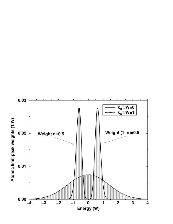
FIG. 1.: Peak weights of the atomic limit spectrum at low and high temperature. Plot is for the (forced) paramagnetic state with $S=J=\infty$, $h=0$, $n=0.5$, $\omega/W=0.05$ and $g/W=0.18$, $W$ being an energy parameter.

FIG. 2.: Suppression of the Curie temperature $T_{\rm C}$ with increasing electron-phonon coupling $g/W$. Plot is for $S=J=\infty$, $h=0$, $n=0.5$ and $\omega/W=0.05$.

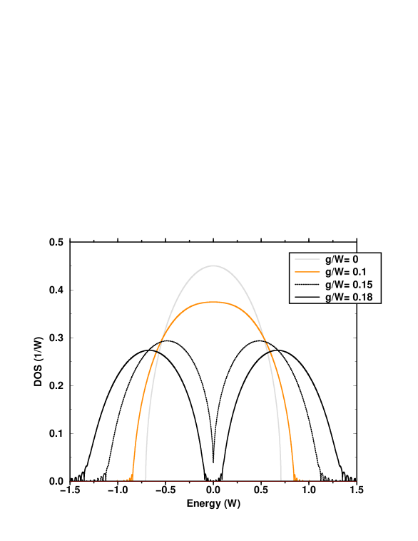
FIG. 3.: Development of the zero-energy pseudogap and subbands in the spectrum with increasing electron-phonon coupling $g/W$. Plot is for the (forced) zero-temperature paramagnetic state with $S=J=\infty$, $h=0$, $n=0.5$ and $\omega/W=0.05$.

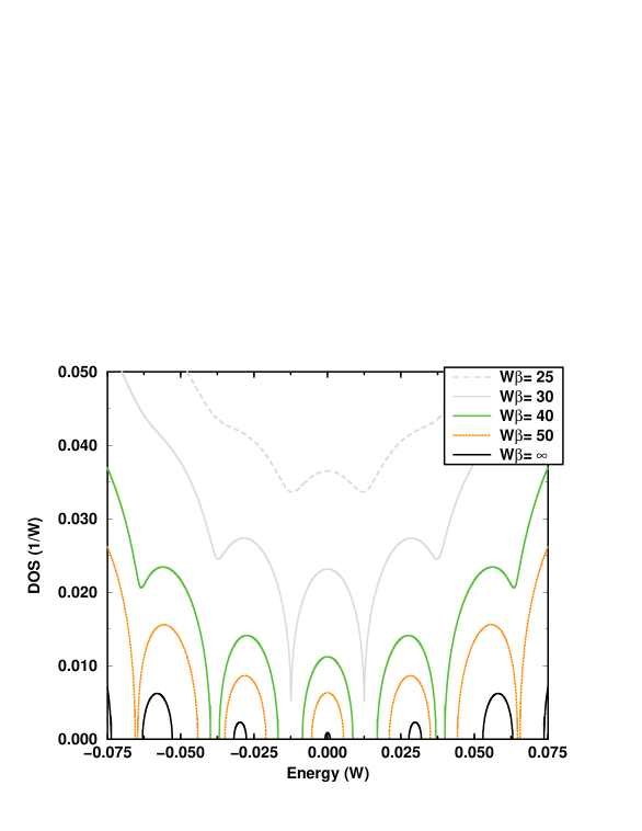
FIG. 4.: Evolution of the subbands in the pseudogap (see Fig. 3) with temperature. Plot is for the (forced) paramagnetic state with $S=J=\infty$, $h=0$, $n=0.5$, $\omega/W=0.05$ and $g/W=0.18$.

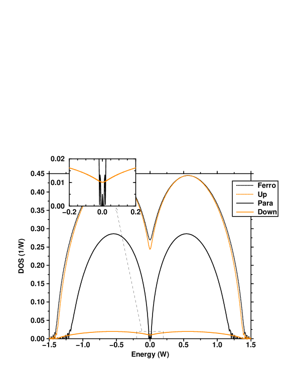
FIG. 5.: Comparison of low-temperature spectra for different magnetisations: saturated ferromagnetism and (forced) paramagnetism for $T=0$ versus calculated up- and down-spin spectra for $k_{\rm B}T=0.005W\ll k_{\rm B}T_{\rm C}$ where $\langle S^{z}\rangle=0.915$. Plot is for $S=J=\infty$, $h=0$, $n=0.5$, $\omega/W=0.05$ and $g/W=0.16$.

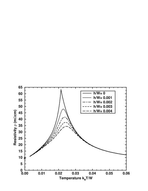
FIG. 6.: Resistivity versus temperature for $S=J=\infty$, $n=0.5$, $\omega/W=0.05$ $g/W=0.16$ and various $h$. The lattice constant $a=5\AA$.

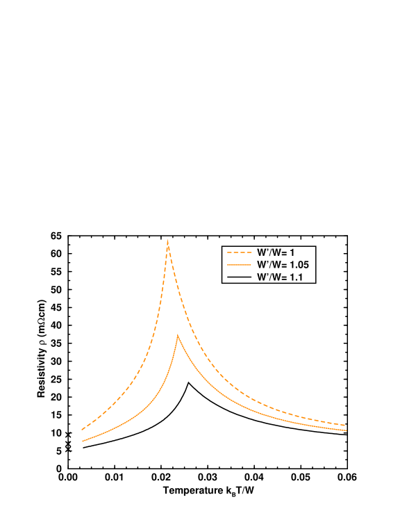
FIG. 7.: Effect of pressure (increasing half-bandwidth $W$) on the resistivity. Plot is for $S=J=\infty$, $n=0.5$, $\omega/W=0.05$ and $g/W=0.16$. The lattice constant $a=5\AA$.

REFERENCES

[1]Email: a.c.green@ic.ac.uk
[2]
H. Röder, J. Zang and A.R. Bishop, Phys. Rev. Lett. 76, 1356
(1996).
[3]
J. Zang, A.R. Bishop and H. Röder, Phys. Rev. B 53, R8840 (1996).
[4]
D.M. Edwards, A.C.M. Green and K. Kubo, J. Phys. Condens. Matter
11, 2791 (1999).
[5]
A.C.M. Green and D.M. Edwards, J. Phys. Condens. Matter 11,
10511 (1999).
[6]
A.J. Millis, R. Mueller and B.I. Shraiman, Phys. Rev. B 54,
5405 (1996).
[7]
A.J. Millis, B.I. Shraiman and R. Mueller,
Phys. Rev. Lett. 77, 175 (1996).
[8]
A.J. Millis, R. Mueller and B.I. Shraiman,
Phys. Rev. B 54, 5389 (1996).
[9]
S. Ciuchi, F. de Pasquale, S. Fratini and D. Feinberg,
Phys. Rev. B 56, 4494 (1997).
[10]
A. Georges, G. Kotliar, W. Krauth and M.J. Rozenberg,
Rev. Mod. Phys. 68, 13 (1996).
[11]
K. Kubo, J. Phys. Soc. Japan 36, 32 (1974).
[12]
H. Sumi, J. Phys. Soc. Japan 36, 770 (1974).
[13]
V. Jani, Z. Phys. B 83, 227 (1991).
[14]
J. Hubbard, Proc. Roy. Soc. 281, 401 (1964).
[15]
G.D. Mahan, Many-Particle Physics Ed.2 (Plenum, New York, 1981)
p. 286
[17]
N. Furukawa, in Physics of Manganites edited by
T.A. Kaplan and S.D. Maharty
(Kluwer Academic/Plenum, New York, 1999), p. 1
[18]
G.M. Zhao, V. Smolyaninova, W. Prellier and H. Keller, cond-mat/9912037
(1999).
[19]
A. Schwartz, M. Scheffler and S.M. Anlage, Phys. Rev. B 61, R870
(2000).
[20]
A.P. Ramirez, J. Phys. Condens. Matter 9, 8171 (1997).
[21]
P. Schiffer, A.P. Ramirez, W. Bao and S-W. Cheong,
Phys. Rev. Lett. 75, 3336 (1995).
[22]
J.J. Neumeier, M.F. Hundley, J.D. Thompson and R.H. Heffner,
Phys. Rev. B 52, R7006 (1995).
[23]
S. Ciuchi, F. de Pasquale, C. Masciovecchio and D. Feinberg,
Europhys. Lett. 24, 575 (1993).