Current bistability and hysteresis in strongly correlated quantum wires

Abstract

Nonequilibrium transport properties are determined exactly for an adiabatically contacted single-channel quantum wire containing one impurity. Employing the Luttinger liquid model with interaction parameter $g$, for very strong interactions, $g\mbox{\raisebox{-4.0pt}{$\,\buildrel<\over{\sim}\,$}}0.2$, and sufficiently low temperatures, we find an S-shaped current-voltage relation. The unstable branch with negative differential conductance gives rise to current oscillations and hysteretic effects. These nonperturbative and nonlinear features appear only out of equilibrium.

Transport in 1D conductors is one of the focal points of condensed matter physics. At low energy scales, such materials have been predicted long ago to behave as Luttinger liquids (LL) instead of Fermi liquids [1]. Over the past few years, several possible experimental realizations of LL behavior have been reported. In particular, narrow quantum wires (QW) in semiconductor heterostructures can be operated in the single-channel limit [2, 3]. Other realizations include quasi-1D materials such as long chain molecules [4], carbon nanotubes [5], or edge states in fractional quantum Hall (FQH) bars [6]. Since the latter are in fact chiral LLs, where right- and left-moving branches are spatially separated, FQH edge state transport [7, 8] is distinct from the case of a quantum wire. In this Letter, we emphasize the important and indeed surprising differences arising for standard (achiral) LL systems characterized by the interaction parameter $g<1$. We focus on the archetype problem of a spinless single-channel QW containing backscattering (BS) by one impurity [7].

Our main results are as follows. The current $I(U,T,g)$ under an applied voltage bias $U$ at temperature $T$ obeys scaling [$I$ depends only on $U$ and $T$ measured in terms of the impurity scale $T_{B}$] and a duality relation connecting the strong and weak BS limits under the simultaneous exchange $g\to 1/g$. Both the scaling function and the duality relation are different from the FQH case and are determined exactly. For very strong interactions, $g\mbox{\raisebox{-4.0pt}{$\,\buildrel<\over{\sim}\,$}}0.2$, and low temperatures, the $I-U$ characteristics is multivalued, containing an unstable branch of negative differential conductance (NDC). Once the QW is embedded in a load circuit, this S-shaped $I(U)$ relation can lead to hysteresis, current switching and self-sustained current oscillations [9]. Such effects could be observed in a QW of very low electron density.

Coupling of QW to voltage bias. — We focus on a QW adiabatically connected to ideal time-independent voltage reservoirs held at electro-chemical potentials $\mu_{1,2}$ [10, 11, 12]. The 1D conductor extending from $-L/2<x<L/2$ is considered to be a LL, with an impurity of BS strength $\lambda$ sitting at $x=0$. This defines $T_{B}=c_{g}\lambda(\lambda/\omega_{c})^{g/(1-g)}$, where $\hbar=k_{B}=1$, $\omega_{c}$ is the electronic bandwidth, and $c_{g}$ is a numerical prefactor of order unity (its precise value is of no interest here and given in Ref.[13]). The Coulomb interactions take the form $H_{I}=(e/2)\int dx\rho(x)\varphi(x)$, where $\rho(x)$ is the electron density and the Poisson equation is replaced by

$$e\varphi(x)=u_{0}\rho(x)\quad{\rm with}\qquad g=(1+u_{0}/\pi v_{F})^{-1/2}\;,$$ (1)

with the Fermi velocity $v_{F}$. Here a screening backgate or other metallic surroundings cause short-ranged interactions within the QW. Since we are dealing with a strongly correlated non-Fermi liquid system, the well-known Landauer approach [10] does not apply. In the past, external voltage sources were often modeled by attaching $g=1$ LLs to the ends of the QW [14], but computations become exceedingly difficult for $\lambda>0$. Therefore we employ the radiative boundary conditions of Ref.[11] which represent the natural extension of Landauer’s original ideas [10] to a strongly correlated 1D metal. Using different arguments, these boundary conditions have been confirmed and generalized to a.c. transport [16, 17].

Let us briefly summarize the main ideas [11, 12]. Suppose one injects the “bare” densities $\rho_{R}^{0}$ and $\rho_{L}^{0}$ at positions $x$ close to the end of the QW. The average density $\rho=\rho_{R}+\rho_{L}$ [we omit the expectation values for brevity] is then self-consistently determined by

$$\rho_{R}(x)+\rho_{L}(x)=\rho_{R}^{0}+\rho_{L}^{0}-e\varphi(x)/\pi v_{F}\;,$$ (2)

since the band bottom shifts by $e\varphi(x)$. With Eq. (1) we then get the local relation $\rho_{R}+\rho_{L}=g^{2}(\rho_{L}^{0}+\rho_{R}^{0})$, in agreement with the compressibility of a LL, $\kappa=g^{2}/\pi v_{F}$. Since screening affects only the total charge, see Eq. (1), we also have $\rho_{R}-\rho_{L}=\rho^{0}_{R}-\rho^{0}_{L}$. Solving these two relations for $\rho^{0}_{R/L}$ and using $\rho_{R}^{0}(-L/2)=\mu_{1}/2\pi v_{F}$ and $\rho_{L}^{0}(L/2)=\mu_{2}/2\pi v_{F}$, we obtain the boundary conditions of Refs.[11, 12, 16],

$$\frac{g^{-2}\pm 1}{2}\rho_{R}(\mp L/2)+\frac{g^{-2}\mp 1}{2}\rho_{L}(\mp L/2)=\pm\frac{U}{4\pi v_{F}}\;,$$ (3)

where we put $\mu_{1}=-\mu_{2}=U/2$ with the applied voltage $U$ and $e=1$. We assume full translational invariance such that the sound velocity $v=v_{F}/g$ (below we set $v=1$). The Sommerfeld-like boundary conditions (3) are imposed at the left/right end of the conductor at long times $t$ where the stationary nonequilibrium state has been reached. Below we assume that the relevant energy scale ($k_{B}T$ or $eU$) exceeds $v/L$, and henceforth take $L\to\infty$.

Exact solution and duality. — Like for the tunneling problem in the FQH effect [8], it is possible to compute exactly the current out of equilibrium. The basic idea is first to fold the problem onto the boundary sine-Gordon model, and then use integrability of the latter [13]. The final equations governing the physics are quite simple. For clarity, we restrict ourselves to the case $g=1/p$ with $p$ integer. The basic quantities are then pseudo-energies $\epsilon_{j}(\theta)$ for rapidity $\theta$, obeying a set of thermodynamic Bethe ansatz (TBA) integral equations,

$$\epsilon_{j}(\theta)=T\sum_{k}N_{jk}\int d\theta^{\prime}{s(\theta-\theta^{\prime})\over 2\pi}\ln\left(1+e^{(\epsilon_{k}(\theta^{\prime})-\mu_{k})/T}\right)\;,$$ (4)

where $s(\theta)=(p-1)/\cosh[(p-1)\theta]$ and $N_{jk}$ is the incidence matrix of the following TBA diagram, on which the labels $j,k$ run:

$\hskip 147.95424pt\bigcirc\hskip 7.11317pt+$ $\hskip 145.10922pt\bigcirc\hskip 8.5359pt-$ $\hskip 136.5733pt\Big{/}$ $\hskip 133.72786pt\Big{\backslash}$ $1\hskip 28.45274pt2\hskip 36.98866pt\hskip 11.38092ptp-3$ $\bigcirc$——$\bigcirc$——$\bigcirc$——$\bigcirc$——$\bigcirc$     $p-2$

Here we have defined parameters for the breathers $m_{j}=2\sin{j\pi\over 2(p-1)}$ with $j=1,\ldots,p-2$, and for the kink and antikink, $m_{\pm}=1$ [8]. The latter are the fundamental charged particles in the integrable description. All the physical particles are coupled by non trivial $S$ matrix elements. However, manipulation of the TBA equations gives rise to the simpler structure of coupling for the pseudoenergies represneted on the foregoing diagram. The chemical potentials are $\mu_{j}=0$ for the $p-2$ breathers, and $\mu_{\pm}=\mp W/2$ for kink and antikink. Here $W$ is determined self-consistently, see below. Having found the $\epsilon$’s, the densities of kinks and antikinks are given by $\sigma_{\pm}=nf_{\pm}$, where the pseudo-energies $\epsilon_{\pm}$ are equal, $2\pi n=d\epsilon_{\pm}/d\theta$, and the filling fractions read

$$f_{\pm}(\theta)=1/\{1+\exp[(\epsilon(\theta)\mp W/2)/T]\}\;.$$ (5)

With these definitions, the final expression for the current reads

$$I=\int\left|T_{++}\right|^{2}(\sigma_{+}-\sigma_{-})\,d\theta\;,$$ (6)

where, with the impurity scale $T_{B}\propto\exp\theta_{B}$ defined above, the tunneling probability is

$$|T_{++}|^{2}=\left(1+\exp[-2\left(g^{-1}-1\right)(\theta-\theta_{B})]\right)^{-1}\;.$$ (7)

The current is implicitly a function of $W$, which is self-consistently determined through

$$\int\left(\left|T_{++}\right|^{2}+\frac{1}{g}\left|T_{+-}\right|^{2}\right)(\sigma_{+}-\sigma_{-})\,d\theta=\frac{U}{2\pi}\;,$$ (8)

where $|T_{+-}|^{2}=1-|T_{++}|^{2}$.

¿From these equations, it is now straightforward to deduce the following identity giving the parameter $W$ in terms of the physical voltage and current,

$$U=2\pi\left(1-{1\over g}\right)I+W$$ (9)

In the sequel, we will also use the quantity

$$V=U-2\pi I=W-2\pi I/g\;,$$ (10)

whose physical meaning is the four-terminal voltage across the impurity [11], i.e., the voltage difference measured by weakly coupled reservoirs on either side of the impurity. We then find that for non-vanishing $T_{B}$, the current interpolates between $I=0$ and (going back to physical units) $I=(e^{2}/h)U$ as the applied voltage $U$ is increased. Similarly, the linear conductance interpolates between the perfectly quantized high-temperature value $G=e^{2}/h$ also found in a clean QW [14], and the vanishing low-temperature ($T\ll T_{B})$ conductance predicted in Ref. [7]. For temperatures above $\omega_{c}$ or $v_{F}/r$, where $r$ is the interaction range, the conductance saturates before reaching $e^{2}/h$ in a real QW.

The above equations can be solved in closed form at vanishing temperature. The solution for arbitrary $g$ is expressed in terms of two different series expansions, depending on whether the impurity BS is weak or strong. In the latter case, we find

$$I = G(p)(e^{A}/\pi)\sum_{n=1}^{\infty}(-1)^{n+1}\frac{\sqrt{\pi}~{}\Gamma(np)}{2\Gamma(n)\Gamma\left(n(p-1)+3/2\right)}$$ (12)

$$\times\left(e^{A+\Delta-\theta_{B}}\right)^{2n(p-1)}\;,$$

while the boundary condition (3) reads

$$U = 2G(p)e^{A}-(p-1)G(p)e^{A}\sum_{n=1}^{\infty}(-1)^{n+1}$$ (14)

$$\times\frac{\sqrt{\pi}~{}\Gamma(np)}{\Gamma(n)\Gamma\left(n(p-1)+3/2\right)}\left(e^{A+\Delta-\theta_{B}}\right)^{2n(p-1)}\;.$$

Here we have introduced the notations $G(p)=p\sqrt{\pi}\Gamma(p/2(p-1))\,/\,\Gamma(1/2(p-1))$ and $\Delta=[\ln(p-1)-p\ln(p)/(p-1)]/2$. The parameter $A$ follows by solving Eq. (14) for a given voltage $U$. Inserting it into Eq. (12) gives the $I-U$ relation and $W=2G(p)e^{A}$. Equations in the weak BS limit follow from the duality relation described below.

The TBA equations are easily solved for any $T$ at $g=1/2$, with the result [12, 18]

$$V(W)=2T_{B}\,{\rm Im}\,\psi\left(\frac{1}{2}+\frac{T_{B}+iW/2}{2\pi T}\right)\;,$$ (15)

where $\psi$ is the digamma function and $T_{B}=\pi\lambda^{2}/\omega_{c}$. The linear conductance is then

$$G(T)=\frac{e^{2}}{h}\,\frac{1-c\psi^{\prime}(\frac{1}{2}+c)}{1+c\psi^{\prime}(\frac{1}{2}+c)}\;,\qquad c\equiv T_{B}/2\pi T\;,$$ (16)

with the trigamma function $\psi^{\prime}(x)$. For high temperatures, this approaches $e^{2}/h$, while it vanishes as $G\sim T^{2}$ at low temperatures. Notably, while this is the same power law as in the FQH effect [7], the prefactor is now different. To get the current for arbitrary values of $g,T$ and $U$, one has to resort to a straightforward numerical solution of the TBA equations (12) and (14). The linear conductance can be given in closed form,

$$G=\frac{e^{2}}{h}\frac{\int\,d\theta\left|T_{++}\right|^{2}df_{\pm}/d\theta}{\int\,d\theta\left(\left|T_{++}\right|^{2}+\left|T_{+-}\right|^{2}/g\right)df_{\pm}/d\theta}\;,$$ (17)

where the filling fractions (5) have to be evaluated at $W=0$.

A remarkable nonperturbative consequence of the TBA equations is the existence of a duality relation for the current valid at any temperature,

$$I(\lambda,U,g)={U\over 2\pi}-I\left(\lambda_{d},U,{1\over g}\right)\;,$$ (18)

where $\lambda_{d}\propto\lambda^{-1/g}$ [13]. This duality is similar but different from the one found in the FQH case [8]. Although, like in the FQH case, quasiparticles of charge $q=ge$ tunnel in the weak BS limit, and electrons with $q=e$ in the strong BS limit, the coupling of the QW to the reservoirs modifies the current and gives rise to the new duality (18).

Bistability regime. — The curves for the linear conductance in a QW are generally similar to those for the FQH effect, with the main difference that the high temperature value is now $e^{2}/h$ independent of $g$. Much more interesting and unexpected physics occurs in the nonlinear out-of-equilibrium regime for very strong interactions and low temperatures. The most direct approach to see this is the quasiclassical limit, $g\ll 1$, at $T=0$, which we consider first. In the bosonized theory, after integrating out the standard boson phase fields away from $x=0$ but taking into account the boundary conditions (3) [12], one is left with the equation of motion

$$d\Phi/dt+g\pi T_{B}\sin\Phi=gW\;,$$ (19)

where $T_{B}=2\lambda$ and the current operator is $\dot{\Phi}/2\pi$. This equation can also be obtained from the explicit solution of the TBA in that limit. For $W>\pi T_{B}$, the current grows proportional to $\Delta=[W^{2}-(\pi T_{B})^{2}]^{1/2}$. This is readily seen from the solution of Eq. (19), which reads in terms of $y=\tan[g\Delta t/2]$,

$\displaystyle\tan(\Phi/2)=Wy(t)/[\Delta+\pi T_{B}y(t)]\;.$

Hence the average over one time period yields

$$\langle I\rangle=\frac{g}{2\pi}\Delta\;\Theta(W-\pi T_{B})\;,$$ (20)

where $\Theta$ is the Heaviside function. The $I(W)$ curve is single-valued, but by inserting the definitions (9) and (10), and eliminating $I$, we see that $U=F(W)$ with

$$F(W)=gW+(1-g)V(W)$$ (21)

can have several solutions $W$. Therefore the $I(U)$ relation is multivalued throughout the regime $U_{1}<U<U_{2}$, where $U_{1}=\sqrt{g(2-g)}\,\pi T_{B}$ and $U_{2}=\pi T_{B}$. The three solutions for the current in this regime are $I=0$ and

$$I_{\pm}(U)=\frac{U}{2\pi(2-g)}\left(1-g\pm\sqrt{1-g(2-g)(\pi T_{B}/U)^{2}}\right)\;.$$ (22)

For $U<U_{1}$, we only get $I=0$, and for $U>U_{2}$, $I_{+}(U)$ is the only allowed solution. Clearly, on the branch $I_{-}(U)$, we have negative differential conductance (NDC), and therefore this branch is unstable. Such S-shaped current-voltage relations are familiar, e.g., in nonlinear semiconductor physics [9] and in charge-density wave transport [19]. By putting the QW into a properly designed load circuit, self-sustained current oscillations can be generated [9]. Furthermore, putting a resistance $R$ in series and applying the voltage $V_{a}$ to the whole circuit, one has

$$V_{a}=RI(U)+U\;,$$ (23)

which can easily be solved for $I(V_{a})$. For $R/(e^{2}/h)>g^{-1}-1$, we get a single-valued $I(V_{a})$ curve, i.e., the NDC branch has been stabilized. For smaller $R$, also the $I(V_{a})$ curve will be multi-valued. In practice, one then gets hysteresis, and the current jumps between two branches (bistability).

How stable is this behavior once thermal and quantum fluctuations are taken into account? Repeating the above $g\ll 1$ calculation for finite temperature with methods from Ref.[20], one finds

$$V(W)=\pi T_{B}\,{\rm Im}\,\frac{I_{1-iW/2\pi T}(T_{B}/2T)}{I_{-iW/2\pi T}(T_{B}/2T)}$$ (24)

with the modified Bessel function $I_{\nu}(z)$ with complex order $\nu$. The high-temperature expansion ($T\gg T_{B}$) of Eq. (24) predicts bistability to occur for all $T<T_{c}(g)$ with

$$T_{c}(g\ll 1)=T_{B}\sqrt{(1-g)/16g}\;.$$ (25)

Therefore as $g\to 0$, the bistability occurs at all temperatures. Bistability is not destroyed by quantum fluctuations either, as can be checked using the exact solution. At $T=0$, one finds that the NDC disappears for $g\approx 0.2$, see Figure 1. This value gets smoothly lowered as temperature increases. We stress that the bistability is a true nonperturbative nonequilibrium phenomenon that has no parallel in the linear conductance [21].

Finally we turn to rather elementary physical reasoning explaining the origin of the predicted bistable behavior independent of the details of our boundary condition. In the presence of impurity BS, a portion $V$ of the voltage drops at the impurity site. Then the average current $\langle I\rangle=(U-V)/2\pi$, where $1/2\pi$ [$=e^{2}/h$ in physical units] is the d.c. conductance of the perfect wire. However, a fluctuation $\delta I$ of the current must obey

$$\delta I=-(g/2\pi)\delta V\;,$$ (26)

with the associated fluctuation $\delta V$ of the four-terminal voltage and the a.c. conductance $g/2\pi$ [7]. Equation (26) reflects the fact that the impurity BS potential $\lambda\cos\Phi$ for the $x=0$ boson field $\Phi$ is due to tunneling of fractional quasiparticles with charge $ge$ [22]. In terms of the boson field, the current is $\langle I\rangle+\delta I=\dot{\Phi}/2\pi$, and the voltage fluctuations read $\delta V=2\pi\lambda\sin\Phi-V$. The first term is basically the derivative of the pinning potential $\lambda\cos\Phi$ [22]. With these relations, it is straightforward to verify the equation of motion (19). The latter describes an overdamped particle moving in the tilted washboard potential $-g(2\pi\lambda\cos\Phi+W\Phi)$, where the bias $W=U+2\pi(g^{-1}-1)\langle I\rangle$ depends explicitly on the current. This feedback mechanism together with the nonlinear pinning potential is responsible for bistability. The above arguments also suggest that our assumption of adiabatic coupling to the reservoirs is not essential for bistability to occur [23].

To conclude, nonequilibrium transport through a spinless single-channel quantum wire containing one impurity has been studied. Using integrability techniques, the exact solution of this interacting transport problem has been given for adiabatically connected reservoirs. We have discovered bistability phenomena in the current for strong interactions that should be observable in state-of-the-art experiments and constitute a hallmark of strongly interacting quantum wires.

We thank L. Balents, M.P.A. Fisher, and F. Guinea for discussions. This work has been supported by the Deutsche Forschungsgemeinschaft (Grant No. GR 638/19-1), by the National Science Foundation under Grants No. PHY-94-07194 and No. PHY-93-57207, and by the DOE.

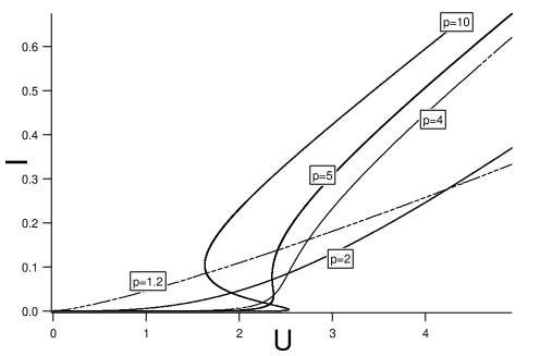
FIG. 1.: Current-voltage relation at $T=0$ for various $g=1/p$. The current is given in units of $(e^{2}/h)T_{B}$, and the voltage in units of $T_{B}$.

REFERENCES

- [1] For a recent perspective, see A.O. Gogolin, A.A. Nersesyan, and A.M. Tsvelik, Bosonization and Strongly Correlated Systems (Cambridge University Press, 1998).
- [2] S. Tarucha, T. Honda, and T. Saku, Solid State Comm. 94, 413 (1995).
- [3] A. Yacoby et al., Phys. Rev. Lett. 77, 4612 (1996).
- [4] V. Vescoli et al., Science 281, 1181 (1998).
- [5] M. Bockrath et al., Nature 397, 598 (1999); Z. Yao et al., ibid. 402, 273 (1999).
- [6] A.M. Chang, L.N. Pfeiffer, and K.W. West, Phys. Rev. Lett. 77, 2538 (1996).
- [7] C.L. Kane and M.P.A. Fisher, Phys. Rev. B 46, 15 233 (1992).
- [8] P. Fendley, A.W.W. Ludwig, and H. Saleur, Phys. Rev. B 52, 8934 (1995); P. Fendley and H. Saleur, Phys. Rev. B 54, 10 845 (1996).
- [9] E. Schöll, Nonequilibrium Phase Transitions in Semiconductors (Springer, Berlin, 1987).
- [10] R. Landauer, IBM J. Res. Dev. 1, 223 (1957); Z. Phys. B 68, 217 (1987).
- [11] R. Egger and H. Grabert, Phys. Rev. Lett. 77, 538 (1996); ibid. 80, 2255(E) (1998).
- [12] R. Egger and H. Grabert, Phys. Rev. B 58, 10 761 (1998).
- [13] A. Koutouza, H. Saleur, and F. Siano, in preparation.
- [14] D.L. Maslov and M. Stone, Phys. Rev. B 52, R5539 (1995); V.V. Ponomarenko, ibid. 52, R8666 (1995); I. Safi and H.J. Schulz, ibid. 52, R17 040 (1995).
- [15] D. Maslov, Phys. Rev. B 52, R14 368 (1995); A. Furusaki and N. Nagaosa, ibid. 54, R5239 (1996).
- [16] I. Safi, Eur. Phys. J B 12, 451 (1999).
- [17] Ya.M. Blanter, F.W.J. Hekking, and M. Büttiker, Phys. Rev. Lett. 81, 1925 (1998).
- [18] Eq. (5.30) in Ref.[12] contains an incorrect numerical factor. The corrected refermionization gives indeed Eq. (15).
- [19] G. Grüner, Density Waves in Solids (Addison-Wesley, Reading, 1994).
- [20] Yu.M. Ivanchenko and L.A. Zil’berman, Zh Eksp. Teor. Fiz. 55, 2395 (1968) [Sov. Phys. JETP 28, 1272 (1969)].
- [21] Spin fluctuations will wash out the bistability. For an experimental check, one has to study a spin-polarized QW.
- [22] C.L. Kane and M.P.A. Fisher, Phys. Rev. Lett. 72, 724 (1994).
- [23] We expect that the relevant part of the plane shrinks as the contact resistance increases.