[

Low-dimensional Bose liquids: beyond the Gross-Pitaevskii approximation

Abstract

The Gross-Pitaevskii approximation is a long-wavelength theory widely used to describe a variety of properties of dilute Bose condensates, in particular trapped alkali gases. We point out that for short-ranged repulsive interactions this theory fails in dimensions $d\leq 2$, and we propose the appropriate low-dimensional modifications. For $d=1$ we analyze density profiles in confining potentials, superfluid properties, solitons, and self-similar solutions.

]

Experimental observation of Bose-Einstein condensation (BEC) in trapped alkali vapors [1] has ushered in a new era of superlow temperature physics. The Gross-Pitaevskii (GP) mean-field theory [2] has proven to be an indispensable tool both in analyzing and predicting the outcome of experiments.

With rapid progress in the experimental exploration of BEC systems it is reasonable to anticipate that effectively one and two-dimensional systems are realistic prospects in the near future [3]. For example, high aspect ratio cigar-shaped traps approximating quasi-one-dimensional BEC systems are already available experimentally [4]. From the theoretical viewpoint low-dimensional systems are rarely well represented by mean-field theories which leads one to question the validity of the GP theory in one and two dimensions. In this paper we shall show that, indeed, the physics of dilute Bose systems requires a fundamental modification of the GP theory in low dimensions $d\leq 2$.

The GP theory is a quasi-classical (or mean-field) approximation which replaces the bosonic field operator $\psi$ by a classical order parameter field $\Phi({\bf r},t)$. For short-ranged interactions the interparticle potential $U({\bf r})$ is replaced by $g\delta^{d}({\bf r})$, where $g$ is the pseudopotential. Then for a system of bosons in an external potential $V$, the energy functional and the equation of motion for $\Phi$ take the following form:

$$F_{GP}=\int d^{d}r\left[{\hbar^{2}\over 2m}|\nabla\Phi|^{2}+V({\bf r})|\Phi|^{2}+{g\over 2}|\Phi|^{4}\right]\ ,$$ (1)

and

$$i\hbar\partial_{t}\Phi={\delta F_{GP}\over\delta\Phi^{*}}=\left[-{\hbar^{2}\over 2m}\nabla^{2}+V({\bf r})+g|\Phi|^{2}\right]\Phi\ .$$ (2)

The GP equations (1) and (2) are widely used to compute a variety of properties of Bose systems [2].

The GP approximation is a long-wavelength theory relying on the concept of the pseudopotential to account for interparticle interactions. However, for repulsive bosons the canonical pseudopotential vanishes in two dimensions [5], implying that an essential modification of the GP theory is necessary for $d\leq 2$. To see how to modify the theory, it is useful to rewrite the last integrand of (1) in terms of the particle density $n=|\Phi|^{2}$, so that $(g/2)|\Phi|^{4}=(g/2)n^{2}$. This can be recognized [2, 6] as the lowest order term of a dilute expansion of the ground-state energy density for $d>2$. Thus the correct low-dimensional local density theory will instead have the ground-state energy density of the $d\leq 2$ dilute Bose system[5, 6], which is not proportional to $n^{2}$.

Let us write the interparticle interaction in the form $U({\bf r})=u_{0}\delta_{a}^{d}({\bf r})$ where $u_{0}$ is the amplitude of the interparticle repulsion, and the notation $\delta_{a}^{d}({\bf r})$ denotes any well-localized function that transforms into the mathematical Dirac $\delta$ function when the range of interaction $a\rightarrow 0$. The renormalization group analysis of this problem [6] reveals that two dimensionless combinations $na^{d}$ and $\hbar^{2}n^{(2-d)/d}/mu_{0}$ play an important role in defining the conditions of the dilute limit for $d\leq 2$.

In the dilute limit $na\ll 1$ and $\hbar^{2}n/mu_{0}\ll 1$, any one-dimensional Bose system with short-ranged repulsive interactions becomes equivalent to a gas of free-fermions [7] (or equivalently point hard-core bosons[8]), with energy density $\pi^{2}\hbar^{2}n^{3}/6m$. This can be generalized[6] for $d<2$ to the statement that for $na^{d}\ll 1$ and $\hbar^{2}n^{(2-d)/d}/mu_{0}\ll 1$, the lowest order term of the ground-state energy density expansion is universal and given by $(\hbar^{2}C_{d}/2m)n^{(2+d)/d}$, where $C_{d}$ is a $d$-dependent constant. This implies that the quartic nonlinearity $|\Phi|^{4}$ in Eq.(1) should be replaced by $|\Phi|^{2(2+d)/d}$. In particular, for the practically important case of one dimension, the system of equations (1) and (2) is modified to

$$F={\hbar^{2}\over 2m}\int dx\left[\left|{d\Phi\over dx}\right|^{2}+{2m\over\hbar^{2}}V(x)|\Phi|^{2}+{\pi^{2}\over 3}|\Phi|^{6}\right]\ ,$$ (3)

and

$$i\hbar\partial_{t}\Phi={\hbar^{2}\over 2m}\left[-\partial_{x}^{2}+{2m\over\hbar^{2}}V(x)+\pi^{2}|\Phi|^{4}\right]\Phi\ .$$ (4)

Similar considerations applied to the marginal two-dimensional case lead to the conclusion that in the dilute limit [5, 6] a theory replacing the GP approximation starts from the energy functional

$$F={\hbar^{2}\over 2m}\int d^{2}r\left[|\nabla\Phi|^{2}+{2m\over\hbar^{2}}V(x)|\Phi|^{2}+{4\pi^{2}\over|\ln(|\Phi|^{2}a^{2})|}|\Phi|^{4}\right]\ .$$ (5)

Ignoring the logarithmic factor will perhaps suffice for many practical purposes; then (5) is precisely of the GP form. Finding an experimental manifestation of the logarithmic correction is likely to be very challenging.

A detailed analytical and numerical study of the one and two-dimensional cases will be given in a longer publication[9]; hereafter we restrict ourselves to only the salient features of one dimension where the deviations from the GP theory are largest.

Density profiles in external potentials: The stationary solution to Eq.(4) defined via $\Phi(x,t)=\phi(x)e^{-i\mu t/\hbar}$ can be found by solving

$${d^{2}\phi\over dx^{2}}+{2m\over\hbar^{2}}(\mu-V(x))\phi-\pi^{2}\phi^{5}=0\ ,$$ (6)

subject to the condition of fixed total particle number $N=\int dx\phi^{2}$ which determines the chemical potential $\mu$. For an external potential that varies slowly on the scale of the interparticle spacing the derivative term in (6) can be ignored: this gives the density profile in the Thomas-Fermi (TF) approximation:

$$n_{TF}(x)=\phi_{TF}^{2}=\left[2m(\mu-V(x))\right]^{1/2}/\pi\hbar\ ,$$ (7)

with the density being zero in the classically forbidden region $\mu<V(x)$. For the practically important case of a harmonic trap, $V=m\omega^{2}x^{2}/2$, and the density profile is elliptical:

$$n_{TF}(x)=\left[(2m\mu-m^{2}\omega^{2}x^{2})\right]^{1/2}/\pi\hbar\ .$$ (8)

The chemical potential is given by $\mu_{TF}=\hbar\omega N$, the density in the center of the trap is $n_{TF}(0)=(2m\hbar\omega N)^{1/2}/\pi\hbar$, and the size of the trapped condensate is $2(2m\hbar\omega N)^{1/2}/\pi\hbar$.

The accuracy of these predictions can be tested against the exact solution of a dilute system of bosons with repulsive interactions: an ideal candidate being a system of point impenetrable bosons. The boson-fermion equivalence[7] implies that in the many-body system, the single-particle energy levels $E_{n}=\hbar\omega(n+1/2)$ of the harmonic oscillator are occupied in a fermionic fashion, i.e. with no more than one particle per state. The chemical potential is then given by $\mu=\hbar\omega(N+1/2)$, which for large $N$ approaches our TF result $\mu_{TF}=\hbar\omega N$. Similarly the density profile can be computed as a sum of squares of the single-particle wave functions:

$$n(x)={1\over(\pi l)^{1/2}}\sum\limits_{k=1}^{N-1}{1\over 2^{k}k!}H_{k}^{2}(x/l)\exp(-x^{2}/l^{2})\ ,$$ (9)

where $H_{k}$ are Hermite polynomials and $l=(\hbar/m\omega)^{1/2}$. The density distribution (9) is plotted in Fig.1 where it is compared with a) the numerical solution of (6) with $V=m\omega^{2}x^{2}/2$, and b) the TF result (8), for different numbers of particles. The main flaw of the theory based on (6) is that it does not reproduce density oscillations due to algebraic ordering of the particles. This is not surprising as (akin to the GP approximation) the discreteness of the particles, which is responsible for the density oscillations, is ignored. Otherwise, the agreement between the approximate and the exact profiles is very good; in the limit of large particle number the differences become imperceptible. These results can be directly tested experimentally; as a comparison we note that the one-dimensional GP theory in the TF approximation predicts [2] $n_{TF}\sim\mu-V(x)$, which is quite distinct from (7), and agrees very poorly with the exact result.

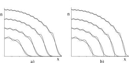
FIG. 1.: The density profile (9) plotted for particle numbers $N=4,9,16,25$ in units $m\omega/\hbar=1$. The non-oscillating curves correspond to a) the numerical solution of (6) and b) the TF result (8).

Solitons: Gray solitons [10] have been recently created and their dynamics was observed in cigar-shaped condensates of ${}^{87}Rb$ vapors [11], which makes it important to understand solitonic properties of the system (3) and (4). Let us look for solutions to (4) (with $V=0$) of the form $\Phi(x,t)=\phi(x,t)e^{-i\mu t/\hbar}$. The function $\phi$ then obeys the equation

$$i\hbar\partial_{t}\phi={\hbar^{2}\over 2m}\left[-\partial_{x}^{2}\phi+\pi^{2}(|\phi|^{4}-\phi_{0}^{4})\phi\right]\ ,$$ (10)

where the chemical potential $\mu=\pi^{2}\hbar^{2}\phi_{0}^{4}/2m$ is selected so that the particle density $n_{0}=\phi_{0}^{2}$ is constant at infinity. In dimensionless variables $f=\phi/\phi_{0}$, $y=\pi n_{0}x$, $\tau=\pi^{2}n_{0}^{2}\hbar t/m$, Eq.(10) simplifies to

$$2i\partial_{\tau}f=-\partial_{y}^{2}f+(|f|^{4}-1)f\ .$$ (11)

We will be looking for a localized traveling wave solution [12] to (11) of the form $f(y,\tau)=f(y-\beta\tau)$ where the dimensionless velocity $\beta$ is measured in units of the sound velocity $c=\pi\hbar n_{0}/m$. This problem can be solved exactly. The results are conveniently described in terms of the amplitude $A$ and phase $\theta$ of the dimensionless order parameter $f=Ae^{i\theta}$:

$$A^{2} = 1-{3(1-\beta^{2})\over 2+(1+3\beta^{2})^{1/2}{\rm cosh}[2(1-\beta^{2})^{1/2}(y-\beta\tau)]}$$ (12)

$$2\theta = {\rm cos}^{-1}\left[{(3\beta^{2}/A^{2})-1\over(1+3\beta^{2})^{1/2}}\right]\ .$$ (13)

The spatial behavior given by (12) is shown in Fig.2.

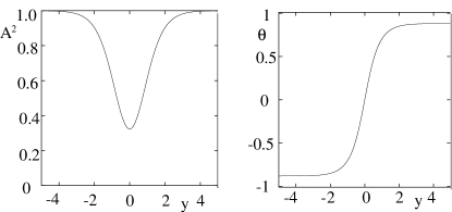
FIG. 2.: The density $A^{2}$ and the phase $\theta$, for the moving soliton (12) with $\beta=1/2$.

The amplitude in (12) describes a moving depression (particle deficit) with the minimal value at the soliton center given by $A^{2}(0)=(1+3\beta^{2})^{1/2}-1$. The soliton exists only for $\beta<1$ (i.e. the soliton velocity cannot exceed the speed of sound); for $\beta=1$ (12) gives the uniform result $A^{2}=1$. On the other hand, for $\beta=0$ (i.e. a vortex, or dark soliton [10]) the minimal value of the amplitude at the soliton center drops to zero.

The phase expressed in (12) varies rapidly in the vicinity of the amplitude dip, staying approximately constant far away from it. The total phase shift across the soliton can be found as $\Delta\theta={\rm cos}^{-1}[(3\beta^{2}-1)/(1+3\beta^{2})^{1/2}]$. It is a continuous function of the soliton velocity varying between $\pi$ (when $\beta=0$) and zero (when $\beta=1$). Antisolitons may be defined as having opposite signs of $d\theta/dy$, and there are no constraints on $\Delta\theta$ for the open line or ring geometries (provided the number of solitons matches the number of antisolitons). However, if there is an imbalance of solitons and antisolitons in the ring geometry, then the uniqueness of the order parameter $f(y,\tau)$ implies that $\Delta\theta$ is a fraction of $2\pi$ for any excess soliton; this will in turn mean that the excess soliton velocity is quantized.

The solution (12) bears some similarity with the one-dimensional soliton of the GP theory [10]; the main qualitative difference (seen after recovering the original units) is that in the dilute limit the soliton size is of order $1/(1-\beta^{2})^{1/2}n_{0}$ independent of the amplitude of the interparticle repulsion [13].

General methods [10] can be used to compute the soliton energy $E$ and momentum $P$. For their dimensionless counterparts $\epsilon=2mE/\pi^{2}\hbar^{2}n_{0}^{2}$ and ${\cal P}=P/\pi\hbar n_{0}$ we find

$$\epsilon = {\surd{3}\over\pi}(1-\beta^{2})\ln\left\{{2+[3(1-\beta^{2})]^{1/2}\over(1+3\beta^{2})^{1/2}}\right\}$$ (14)

$${\cal P} = -{\beta\over(1-\beta^{2})}\epsilon+{1\over\pi}{\rm cos}^{-1}\left[{3\beta^{2}-1\over(1+3\beta^{2})^{1/2}}\right]\ .$$ (15)

The dependencies $\epsilon(\beta)$ and ${\cal P}(\beta)$ parametrically define the soliton dispersion law $\epsilon({\cal P})$ which should be identified [14] with the “hole” branch of the elementary excitations spectrum [15]. To assess the accuracy of $\epsilon({\cal P})$ given in (14) we compare it with the exact result of Lieb[15] for the system of $\delta$-interacting bosons in the dilute limit $\hbar^{2}n/mu_{0}\ll 1$: $\epsilon_{\rm exact}({\cal P})=2|{\cal P}|-{\cal P}^{2}$, for $|{\cal P}|\leq 1$. Since the velocity $\beta$ in (14) varies between zero and unity, the momentum (which we choose to be positive) computed from (14) varies between unity and zero in correspondence with the exact result. It is straightforward to show that for ${\cal P}\ll 1$, the elimination of $\beta$ in (14) leads to $\epsilon=2{\cal P}$ which is again in agreement with the exact result. The behavior $\epsilon({\cal P})$ implied by (14) in the vicinity of the end-point of the spectrum ${\cal P}=1$ is qualitatively similar, and quantitatively close to the exact dependence. To illustrate these statements we have plotted the dispersion law (14) in Fig.3 against the exact result.

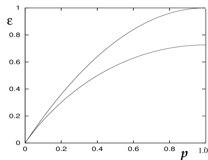
FIG. 3.: The spectrum parameterized by (14) (lower curve) compared to the exact result of Lieb (upper curve).

Superflow: The dimensionless current density is given by $j=A^{2}\partial_{y}\theta$, and below we look for solutions with fixed given current $j$ (i.e. the steady state) and $\partial_{\tau}A=\partial_{\tau}\theta=0$. Substituting $f=Ae^{i\theta}$ and $j=A^{2}d\theta/dy$ into (11), and imposing fixed chemical potential, we find:

$${d^{2}A\over dy^{2}}={j^{2}\over A^{3}}+A^{5}-A\ .$$ (16)

In the spatially uniform state ${d^{2}A\over dy^{2}}=0$ and one finds the dimensionless amplitude $A_{\infty}^{4}=[1+(1-4j^{2})^{1/2}]/2$, which implies that superflow reduces the amplitude of the order parameter. The uniform solution, and thus superfluidity, cease to exist above the critical flow $j_{c}=1/2$ when the amplitude drops down to its minimal value $A_{\infty}^{c}=2^{-1/4}$. These results imply that the critical velocity for superfluidity in the original units is $c/\surd{2}$.

The equation (16) also has an immobile well-localized solution in the form of a dip of the order parameter; far away from the dip the amplitude recovers to its uniform value. The dip solution is closely related to the soliton previously discussed. Indeed, in the reference frame moving with the flow, the dip solution is moving and thus is identical to a soliton. The functional form of the dip can be deduced from (12) by replacing $\beta$ by $j/A_{\infty}^{4}$, $A$ by $A/A_{\infty}$, and $(y-\beta\tau)$ by $yA_{\infty}^{2}$. The dip solution disappears altogether for $j>j_{c}$.

Self-similar solutions: The results derived so far have their counterparts in the context of the one-dimensional GP approximation. However the theory based on Eqs.(3) and (4) allows self-similar solutions which do not exist in the one-dimensional GP theory [16]. Below we only look at the cases consistent with the condition of conservation of total particle number. Consider the system of bosons placed in a harmonic trap. In dimensionless variables it is described by

$$2i\partial_{\tau}f=-\partial_{y}^{2}f+[|f|^{4}+w^{2}y^{2}]f\ ,$$ (17)

where $w=m\omega/\pi^{2}\hbar n_{0}^{2}$ is the dimensionless oscillator frequency ($n_{0}$ now has the meaning of a density introduced to make $f$ dimensionless; it should be determined from the complete solution of the problem). In contrast to (11) (and without loss of generality) we have shifted the origin of the chemical potential. The self-similar solution $f=Ae^{i\theta}$ derived from (17) has the form [16]

$$A=\rho(\tau)^{-1/2}h(y/\rho(\tau))\ ,\ \ \ \theta=\theta_{0}(\tau)+{1\over 2}{d\ln\rho\over d\tau}y^{2}\ ,$$ (18)

where the functions $\rho(\tau)$ and $h(v)$ obey the equations

$${d^{2}\rho\over d\tau^{2}} = -w^{2}\rho+{\gamma\over\rho^{3}}$$ (19)

$${d^{2}h\over dv^{2}} = -\delta h+h^{5}+\gamma v^{2}h$$ (20)

where $\gamma$ and $\delta$ are arbitrary constants. Eq.(20) for the scaling function $h(v)$ has localized solutions only for $\delta>0$ and $\gamma\geq 0$: for $\gamma=0$ an explicit analytic solution to (20) can be written down, while for $\gamma>0$, (20) has the same functional form as the equation we encountered in determining the density profile in the harmonic trap (cf. (6) for $V=m\omega^{2}x^{2}/2$].

The dynamics of the length scale $\rho(\tau)$ can be understood by viewing (19) as a fictitious classical mechanics problem in the potential $U=w^{2}\rho^{2}/2+\gamma/2\rho^{2}$. This analogy implies that an initially localized cloud of bosons in free space ($w=0$) will expand asymptotically in a ballistic fashion: $\rho(\tau)\sim\tau$. In the presence of the confining potential ($w\neq 0$) the scale $\rho(\tau)$ oscillates between maximum and minimum values: for $\gamma=0$ the dynamics of $\rho$ is the same as for a harmonic oscillator of frequency $w$.

We have also performed direct numerical integration of the non-linear equation (4), and have confirmed the existence of both the similarity solutions, and moving trains of solitons with quantized velocity, with amplitude and phase as given by (12). More details will be given in a future publication[9].

In conclusion we have presented a new continuum description of dilute Bose liquids appropriate for low dimensional systems. For the case of one dimension, we have derived stationary properties, along with solitonic and similarity solutions. In particular, the latter have no analog in the GP theory. It is our hope that these results will be testable in BEC experiments in the near future.

REFERENCES

- [1] M. H. Anderson, J. R. Ensher, M. R. Matthews, C. E. Wieman, and E. A. Cornell, Science, 269, 198 (1995); C. C. Bradley, C. A. Sackett, J. J. Tollett, and R. G. Hulet, Phys. Rev. Lett., 75, 1687 (1995); K. B. Davis, M.-O. Mewes, M. R. Andrews, H. J. van Druten, D. S. Durfee, D. M. Kurn, and W. Ketterle, Phys. Rev. Lett., 75, 3969 (1995).
- [2] L. P. Pitaevskii, Zh. Eksp. Teor. Fiz., 40, 646 (1961) [Sov. Phys. JETP, 13, 451 (1961)]; E. P. Gross, Nuovo Cimento, 20, 454 (1961); F. Dalfovo, S. Giorgini, L. P. Pitaevskii, and S. Stringari, Rev. Mod. Phys., 71, 463 (1999), and references therein.
- [3] A. D. Jackson, G. M. Kavoulakis, and C. J. Pethick, Phys. Rev. A, 58, 2417 (1998).
- [4] M. R. Andrews, M.-O. Mewes, N. J. van Druten, D. S. Durfee, D. M. Kurn, and W. Ketterle, Science, 273, 84 (1996).
- [5] M. Schick, Phys. Rev. A, 3, 1067 (1971).
- [6] E. B. Kolomeisky and J. P. Straley, Phys. Rev. B, 46, 11749 (1992).
- [7] M. Girardeau, J. Math. Phys., 1, 516 (1960); E. H. Lieb and W. Liniger, Phys. Rev., 130, 1605 (1963).
- [8] This equivalence was also emphasized by M. Olshanii, Phys. Rev. Lett., 81, 938 (1998).
- [9] E. B. Kolomeisky, T. J. Newman, J. P. Straley, and X. Qi, in preparation.
- [10] Y. S. Kivshar and B. Luther-Davies, Phys. Rep., 298, 81 (1998), and references therein.
- [11] S. Burger, K. Bongs, S. Dettmer, W. Ertmer, K. Sengstock, A. Sanpera, G. V. Shlyapnikov, and M. Lewenstein, cond-mat/9910487.
- [12] A related mathematical problem with extra attractive interaction in the energy functional was considered by I. V. Barashenkov and V. G. Makhankov, Phys. Lett. A, 128, 52 (1988); however, the amplitude of the attraction was not allowed to drop below a certain value.
- [13] The difference between the dark GP soliton and an exact soliton of the system of point impenetrable bosons was recently emphasized by M. D. Girardeau and E. M. Wright, cond-mat/0002062.
- [14] M. Ishikawa and T. Takayama, J. Phys. Soc. Jap., 49, 1242 (1980).
- [15] E. H. Lieb, Phys. Rev., 130, 1616 (1963).
- [16] A. Rybin, G. Varzugin, M. Lindberg, J. Timonen, and R. K. Bullough, cond-mat/0001059.