Effect of Magnetic field on the Pseudogap Phenomena
in High-$T_{{\rm c}}$ Cuprates

1 Introduction

Since the discovery of high-temperature (High-$T_{{\rm c}}$) superconductivity by Bednortz and M$\rm{\ddot{u}}$ller, ${}^{\hbox{\immediate{\bf{?}})}}$ the anomalous normal state properties have been studied for many years from the various points of view.

In particular, the pseudogap phenomena in under-doped cuprates have been recognized as one of the most important issues. There are enormous studies for the issue from both experimental and theoretical points of view. However, the complete understanding still remains to be obtained.

The pseudogap phenomena mean the suppression of the spectral weight near the Fermi energy without any long range order. They are universal phenomena observed in various compounds of under-doped cuprates.

Various experiments such as nuclear magnetic resonance (NMR), ${}^{\hbox{\immediate{\bf{?}})}}$ optical conductivity, ${}^{\hbox{\immediate{\bf{?}})}}$ transport, ${}^{\hbox{\immediate{\bf{?}})}}$ angle-resolved photo-emission spectroscopy (ARPES), ${}^{\hbox{\immediate{\bf{?}})}}$ tunneling spectroscopy, ${}^{\hbox{\immediate{\bf{?}})}}$ electronic specific heat, ${}^{\hbox{\immediate{\bf{?}})}}$ and so on have indicated the existence of the pseudogap in the normal state High-$T_{{\rm c}}$ cuprates from optimally-doped to under-doped region. In particular, NMR measurements of $1/T_{1}T$ have shown the existence of the pseudogap in the spin excitation channel from early years. ${}^{\hbox{\immediate{?})}}$

In the previous paper, we have explained the pseudogap phenomena as a precursor of the strong coupling superconductivity. ${}^{\hbox{\immediate{\bf{?}})}}$ Since the effective Fermi energy $\varepsilon_{{\rm F}}$ is renormalized by the electron-electron correlation, the ratio $T_{{\rm c}}/\varepsilon_{{\rm F}}$ increases in the strongly correlated electron systems. The ratio indicates the strength of the superconducting coupling. Therefore, the strong coupling superconductivity has a general importance for the superconductivity in the strongly correlated electron systems. Moreover, it is natural to consider the strong coupling superconductivity in High-$T_{{\rm c}}$ cuprates because of the high critical temperature $T_{{\rm c}}$ itself. The strong coupling superconductivity necessarily leads to the strong thermal superconducting fluctuations. Such strong fluctuations in the quasi-two dimensional systems have serious effects on the electronic state and give rise to the pseudogap phenomena. ${}^{\hbox{\immediate{?})}}$

Actually, various experiments have indicated the close relationship between the pseudogap phenomena and the superconductivity. In particular, ARPES have directly shown the pseudogap in the one-particle spectral weight ${}^{\hbox{\immediate{?})}}$ and suggested its close relevance and continuity to the superconducting gap. ${}^{\hbox{\immediate{\bf{?}})}}$

Other scenarios have been theoretically proposed for the pseudogap phenomena. In the resonating valence bond (RVB) theory, there are two distinct excitations, spinon and holon. The pseudogap is described as a spinon pairing (so-called ’spin gap’). ${}^{\hbox{\immediate{\bf{?}})}}$ The magnetic scenarios based on the anti-ferromagnetic or SDW gap formation or their precursor have been proposed by various authors. ${}^{\hbox{\immediate{\bf{?}})}}$

Furthermore, the pairing scenarios as a precursor of the superconductivity are classified into several types. The phase fluctuation scenarios have been proposed by Emery and Kivelson ${}^{\hbox{\immediate{\bf{?}})}}$ and calculated by various authors. ${}^{\hbox{\immediate{\bf{?}})}}$ The scenario based on the strong coupling superconductivity has been proposed ${}^{\hbox{\immediate{\bf{?}})}}$ on the basis of the famous Nozi$\grave{{\rm e}}$res and Schmitt-Rink formalism. ${}^{\hbox{\immediate{\bf{?}})}}$ The Nozi$\grave{{\rm e}}$res and Schmitt-Rink formalism is justified in the low density limit. However, the nearly half-filled lattice system should be regarded as a rather high density case. Therefore, the Nozi$\grave{{\rm e}}$res and Schmitt-Rink formalism cannot be applied to the pseudogap phenomena in High-$T_{{\rm c}}$ cuprates. Our scenario is based on the strong coupling superconductivity, but is different from the Nozi$\grave{{\rm e}}$res and Schmitt-Rink formalism. We think of the pseudogap as the gap brought about by the resonance scattering ${}^{\hbox{\immediate{\bf{?}},\penalty 1000\hskip 0.91003pt plus 0.70004pt minus 0.70004pt{\bf{?}})}}$ with the strong superconducting fluctuations. The strong superconducting fluctuations necessarily exist in case of the strong coupling superconductivity in the quasi-two dimensional systems. We have shown that the pseudogap phenomena are naturally understood on the basis of the resonance scattering scenario. ${}^{\hbox{\immediate{?})}}$

Recently, the magnetic field effects on the NMR spin-lattice relaxation rate $1/T_{1}$ have been measured and discussed by several groups to determine the correct scenarios for the pseudogap phenomena .${}^{\hbox{\immediate{\bf{?}},\penalty 1000\hskip 0.91003pt plus 0.70004pt minus 0.70004pt{\bf{?}},\penalty 1000\hskip 0.91003pt plus 0.70004pt minus 0.70004pt{\bf{?}})}}$ The experimental results are interpreted as follows. The magnetic field effects cannot be observed in under-doped cuprates in which the strong pseudogap phenomena occurs in the wide temperature region. ${}^{\hbox{\immediate{?},\penalty 1000\hskip 0.91003pt plus 0.70004pt minus 0.70004pt{?})}}$ In particular, the onset temperature $T^{*}$ does not vary. On the other hand, the magnetic field effects are visible from optimally-doped to slightly over-doped cuprates in which only the weak pseudogap phenomena are observed in the narrow temperature region. ${}^{\hbox{\immediate{?},\penalty 1000\hskip 0.91003pt plus 0.70004pt minus 0.70004pt{\bf{?}})}}$ The observed magnetic field dependences are explained by the conventional weak coupling theory. ${}^{\hbox{\immediate{\bf{?}},\penalty 1000\hskip 0.91003pt plus 0.70004pt minus 0.70004pt{?})}}$ However, for the under-doped cuprates, we have no theoretical explanation of the magnetic field effects on the pseudogap phenomena.

In this paper, we point out that the magnetic field effects are naturally and continuously understood from under-doped to over-doped cuprates on the basis of our resonance scattering scenario. In particular, there is an interpretation that regards the experimental results for under-doped systems as a negative evidence for the pairing scenario. ${}^{\hbox{\immediate{?})}}$ Our results conclude that this interpretation is inappropriate. It is generally considered that the superconducting fluctuations are remarkably influenced by the magnetic field, while the effects of the magnetic field on the spin-fluctuations are considered to be small. Therefore, the experimental results may be interpreted as an evidence for the magnetic scenario for the pseudogap. The misinterpretation is caused by the loss of the understanding for the strong coupling superconductivity. Therefore, we give an explanation for the magnetic field effects on the pseudogap phenomena on the basis of the strong coupling superconductivity. Actually, the experimental results including their doping dependence rather support our scenario for the pseudogap phenomena. ${}^{\hbox{\immediate{?})}}$

This paper is constructed as follows. In §2, we give a model Hamiltonian and explain the theoretical framework adopted in this paper. In §3, we explicitly calculate the single particle self-energy ${\mit{\it\Sigma}}^{{\rm R}}(\mbox{\boldmath$k$},\omega)$, density of states $\rho(\varepsilon)$, NMR spin-lattice relaxation rate $1/T_{1}T$ and their magnetic field dependences. In §4, we discuss the transport phenomena in the pseudogap phase. In §5, we summarize the obtained results and give discussions.

2 Theoretical Framework

In this section, we describe the theoretical framework in this paper. We calculate the magnetic field effects on the pseudogap phenomena by using the same formalism as is used in our previous paper. ${}^{\hbox{\immediate{?})}}$ Therefore, in the first subsection §2.1, we briefly explain the formalism and show the outline of the obtained results in ref.8. In the second subsection §2.2, we introduce the magnetic field effects thorough the Landau quantization and give a rough estimate for the effects. Hereafter, we adopt the unit $\hbar=c=k_{{\rm B}}=1$.

2.1 Pseudogap phenomena under zero magnetic field

We adopt the following two-dimensional model Hamiltonian which has a $d_{x^{2}-y^{2}}$-wave superconducting ground state, with High-$T_{{\rm c}}$ cuprates in mind.

$$H=\sum_{\mbox{\boldmath$k$},s}\varepsilon_{\mbox{\boldmath$k$}}c_{\mbox{\boldmath$k$},s}^{{\dagger}}c_{\mbox{\boldmath$k$},s}+\sum_{\mbox{\boldmath$k$},\mbox{\boldmath$k^{\prime}$},\mbox{\boldmath$q$}}V_{\mbox{\boldmath$k$}-\mbox{\boldmath$q$}/2,\mbox{\boldmath$k^{\prime}$}-\mbox{\boldmath$q$}/2}c_{\mbox{\boldmath$q$}-\mbox{\boldmath$k^{\prime}$},\downarrow}^{{\dagger}}c_{\mbox{\boldmath$k^{\prime}$},\uparrow}^{{\dagger}}c_{\mbox{\boldmath$k$},\uparrow}c_{\mbox{\boldmath$q$}-\mbox{\boldmath$k$},\downarrow},$$ (2.1)

where $V_{\mbox{\boldmath$k$},\mbox{\boldmath$k^{\prime}$}}$ is the $d_{x^{2}-y^{2}}$-wave separable pairing interaction,

$$V_{\mbox{\boldmath$k$},\mbox{\boldmath$k^{\prime}$}}=g\varphi_{\mbox{\boldmath$k$}}\varphi_{\mbox{\boldmath$k^{\prime}$}},$$ (2.2)

$$\varphi_{\mbox{\boldmath$k$}}=\cos k_{x}-\cos k_{y}.$$ (2.3)

Here, $g$ is negative. $\varphi_{\mbox{\boldmath$k$}}$ is the $d_{x^{2}-y^{2}}$-wave form factor.

We consider the dispersion $\varepsilon_{\mbox{\boldmath$k$}}$ given by the tight-binding model for a square lattice including the nearest- and next-nearest-neighbor hopping $t$, $t^{\prime}$, respectively,

$$\varepsilon_{\mbox{\boldmath$k$}}=-2t(\cos k_{x}+\cos k_{y})+4t^{\prime}\cos k_{x}\cos k_{y}-\mu.$$ (2.4)

We fix the lattice constant $a=1$. We adopt $t=0.5\rm{eV}$ and $t^{\prime}=0.45t$. These parameters well reproduce the Fermi surface of the typical High-$T_{{\rm c}}$ cuprates, ${\rm Y}{\rm Ba}_{2}{\rm Cu}_{3}{\rm O}_{6+\delta}$ and ${\rm Bi}_{2}{\rm Sr}_{2}{\rm Ca}{\rm Cu}_{2}{\rm O}_{8+\delta}$. We choose the chemical potential $\mu$ so that the filling $n=0.9$. This filling corresponds to the hole doping $\delta=0.1$. The Fermi surface is shown in Fig.1.

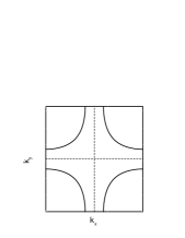
Fig.  1: The Fermi surface adopted in this paper.

In reality, the origin of the pairing interaction should be considered to be the anti-ferromagnetic spin fluctuations. ${}^{\hbox{\immediate{\bf{?}},\penalty 1000\hskip 0.91003pt plus 0.70004pt minus 0.70004pt{\bf{?}})}}$ The spin fluctuations not only cause the pairing interaction but also affect the electronic state. ${}^{\hbox{\immediate{?},\penalty 1000\hskip 0.91003pt plus 0.70004pt minus 0.70004pt{?},\penalty 1000\hskip 0.91003pt plus 0.70004pt minus 0.70004pt{\bf{?}},\penalty 1000\hskip 0.91003pt plus 0.70004pt minus 0.70004pt{\bf{?}})}}$ There are studies dealing with the pairing correlation arising from the spin fluctuations on the basis of the fluctuation exchange (FLEX) approximation. ${}^{\hbox{\immediate{\bf{?}},\penalty 1000\hskip 0.91003pt plus 0.70004pt minus 0.70004pt{\bf{?}})}}$ However, we do not introduce these effects because these details do not seriously affect the pseudogap phenomena as a precursor of the $d_{x^{2}-y^{2}}$-wave superconductivity. There is a feedback effect on the pairing interaction arising from the pseudogap. The pseudogap affects the low frequency component of the spin fluctuations. However, the pairing interaction is mainly caused by the high frequency component of the spin fluctuations. Therefore, we can neglect the feedback effect on the pairing interaction and start from the model with an attractive interaction.

The superconducting fluctuations are expressed by the T-matrix (Fig.2),

$$t(\mbox{\boldmath$q$},{\rm i}\Omega_{n})^{-1} = g^{-1}+\chi_{0}(\mbox{\boldmath$q$},{\rm i}\Omega_{n}),$$ (2.5)

$$\chi_{0}(\mbox{\boldmath$q$},{\rm i}\Omega_{n}) = T\sum_{\mbox{\boldmath$k^{\prime}$},\omega_{m}}{\mit{\it G}}(\mbox{\boldmath$k^{\prime}$},{\rm i}\omega_{m}){\mit{\it G}}(\mbox{\boldmath$q$}-\mbox{\boldmath$k^{\prime}$},{\rm i}\Omega_{n}-{\rm i}\omega_{m})\varphi_{\mbox{\boldmath$k^{\prime}$}-\mbox{\boldmath$q$}/2}^{2}.$$ (2.6)

Here, $\omega_{m}=2\pi(m+\frac{1}{2})T$ and $\Omega_{n}=2\pi nT$ are the fermionic and bosonic Matsubara frequencies, respectively.

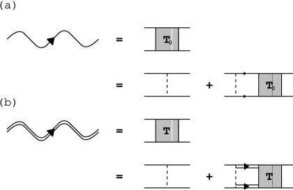
Fig.  2: The scattering vertex represented by the ladder diagrams in the particle-particle channel (T-matrix). The dashed lines represent the attractive interaction. The single and double solid lines represent the propagators of the bare and renormalized fermions, respectively. The single and double wavy lines represent the propagators of the bare and renormalized fluctuating Cooper pairs, respectively.

Here, the scattering vertex arising from the superconducting fluctuations, $\Gamma(\mbox{\boldmath$k$},\mbox{\boldmath$q$}-\mbox{\boldmath$k$}:\mbox{\boldmath$k^{\prime}$},\mbox{\boldmath$q$}-\mbox{\boldmath$k^{\prime}$}:{\rm i}\Omega_{n})$ is factorized into $\Gamma(\mbox{\boldmath$k$},\mbox{\boldmath$q$}-\mbox{\boldmath$k$}:\mbox{\boldmath$k^{\prime}$},\mbox{\boldmath$q$}-\mbox{\boldmath$k^{\prime}$}:{\rm i}\Omega_{n})=\varphi_{\mbox{\boldmath$k$}-\mbox{\boldmath$q$}/2}t(\mbox{\boldmath$q$},{\rm i}\Omega_{n})\varphi_{\mbox{\boldmath$k^{\prime}$}-\mbox{\boldmath$q$}/2}$. The form factor $\varphi_{\mbox{\boldmath$k$}}$ in the above expression gives rise to the $d_{x^{2}-y^{2}}$-wave shape of the pseudogap.

When $1+g\chi_{0}(\mbox{\boldmath$0$},0)=0$, $t(\mbox{\boldmath$0$},0)$ diverges and the superconductivity occurs. This is the famous Thouless criterion which is equivalent to that of the BCS theory in the weak coupling limit. ${}^{\hbox{\immediate{?})}}$ Analytically continued T-matrix $t(\mbox{\boldmath$q$},\Omega)$ can be regarded as a propagator of the fluctuating Cooper pairs.

Here, we are interested in the normal state near the superconducting critical point, where the superconducting fluctuations are enhanced. There, $1+g\chi_{0}(\mbox{\boldmath$0$},0)$ is small and $t(\mbox{\boldmath$q$},\Omega)$ is strongly enhanced around $\mbox{\boldmath$q$}=\Omega=0$. Even in the weak coupling limit, there are corrections on the various quantities due to the superconducting fluctuations. They are well known as the Aslamazov-Larkin term (AL term) ${}^{\hbox{\immediate{\bf{?}})}}$ and the Maki-Thompson term (MT term). ${}^{\hbox{\immediate{\bf{?}})}}$ These terms are the corrections on the two-body correlation function. On the other hand, the superconducting fluctuations more seriously affect the one-particle electronic states in the strong or intermediate coupling region. The superconducting fluctuations give rise to the pseudogap phenomena. The weak correction on the density of states (DOS correction term) has been discussed for High-$T_{{\rm c}}$ cuprates within the weak coupling theory. ${}^{\hbox{\immediate{?},\penalty 1000\hskip 0.91003pt plus 0.70004pt minus 0.70004pt{\bf{?}})}}$ Our calculation corresponds to an extension of these weak coupling theories to the strong coupling ones.

Because $t(\mbox{\boldmath$q$},\Omega)$ is strongly enhanced around $\mbox{\boldmath$q$}=\Omega=0$, its main contribution to the single particle self-energy ${\mit{\it\Sigma}}(\mbox{\boldmath$k$},\omega)$ originates from the vicinity of $\mbox{\boldmath$q$}=\Omega=0$. Therefore, we expand $t^{-1}(\mbox{\boldmath$q$},\Omega)$ in the vicinity of $\mbox{\boldmath$q$}=\Omega=0$. This expansion corresponds to the time-dependent-Ginzburg-Landau (TDGL) expansion.

$$gt^{-1}(\mbox{\boldmath$q$},\Omega)=t_{0}+b\mbox{\boldmath$q$}^{2}-(a_{1}+{\rm i}a_{2})\Omega.$$ (2.7)

The properties of the TDGL parameters are discussed in detail in our previous paper. ${}^{\hbox{\immediate{?})}}$ The outline is the following. As is described above, $t_{0}=1+g\chi_{0}(\mbox{\boldmath$0$},0)$ is $0$ at the critical point and is sufficiently small in the vicinity of the critical point. The parameter $b$ is generally related to the coherence length $\xi_{0}$, $b\propto\xi_{0}^{2}$. The parameter $a_{2}$ express the time scale of the fluctuations. Roughly speaking, the parameters $a_{2}$ and $b$ are described as

$$a_{2}\propto\rho_{{\rm d}}(0)/T_{{\rm c}}$$

$$b\propto\rho_{{\rm d}}(0)/T_{{\rm c}}^{2}.$$ (2.8)

Here, we have defined the effective density of states for the $d_{x^{2}-y^{2}}$-wave symmetry, $\rho_{{\rm d}}(\varepsilon)=\sum_{\mbox{\boldmath$k$}}\rho_{\mbox{\boldmath$k$}}(\varepsilon)\varphi_{\mbox{\boldmath$k$}}^{2}$, where, $\rho_{\mbox{\boldmath$k$}}(\varepsilon)$ is the one-particle spectral weight $\rho_{\mbox{\boldmath$k$}}(\varepsilon)=A_{\mbox{\boldmath$k$}}(\varepsilon)=-\frac{1}{\pi}{\rm Im}{\mit{\it G}}^{{\rm R}}(\mbox{\boldmath$k$},\varepsilon)$. It should be noticed that $\rho_{{\rm d}}(\varepsilon)$ is more sensitive to the pseudogap formation rather than the usual density of states $\rho(\varepsilon)=\sum_{\mbox{\boldmath$k$}}\rho_{\mbox{\boldmath$k$}}(\varepsilon)$.

Because of the high critical temperature $T_{{\rm c}}$ and the renormalization effect by the pseudogap, both $a_{2}$ and $b$ are strongly reduced in the strong coupling superconductivity. These features indicate that the scattering vertex due to the superconducting fluctuations is strongly enhanced. Although the T-matrix calculation used in this paper does not include the renormalization effect, these behaviors are obtained qualitatively.

On the other hand, $a_{1}$ is not so reduced by the strong coupling superconductivity. Especially, High-$T_{{\rm c}}$ cuprates have a comparatively large value of $a_{1}$ because of their strong particle-hole asymmetry. Therefore, we cannot neglect $a_{1}$, although it is usually neglected in the weak coupling theories. ${}^{\hbox{\immediate{\bf{?}})}}$

In the T-matrix calculation, we estimate the TDGL parameters by using the non-interacting Green function ${\mit{\it G}}^{(0){\rm R}}(\mbox{\boldmath$k$},\omega)=(\omega-\varepsilon_{\mbox{\boldmath$k$}}+{\rm i}\delta)^{-1}$ (Fig.2(a)). This estimation corresponds to the Gauss approximation for the superconducting fluctuations. The critical temperature is determined in the mean field level, $T_{{\rm c}}=T_{{\rm MF}}$. As will be discussed in §5, the self-consistent T-matrix calculation includes the somewhat critical fluctuations (Figs.2(b) and 11). However, fundamental features do not change.

As is minutely described in the previous paper ,${}^{\hbox{\immediate{?})}}$ the resonance scattering by the strong superconducting fluctuations gives rise to the pseudogap on both the one-particle spectral weight and the density of states.

In this paper we describe these features by using the T-matrix calculation (Fig.3(a)). Although we pointed out the several important points in the self-consistent T-matrix calculation (Fig.3(b)), the pseudogap is properly described within the T-matrix calculation. ${}^{\hbox{\immediate{?})}}$

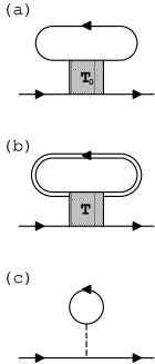
Fig.  3: The diagrams of the single particle self-energy based on (a) the T-matrix approximation calculated in this paper and (b) the self-consistent T-matrix approximation, respectively. (c) The Hartree-Fock term which we exclude. We consider that this term is included in the dispersion relation $\varepsilon_{\mbox{\boldmath$k$}}$ from the beginning.

In the T-matrix calculation, the self-energy is given by

$${\mit{\it\Sigma}}(\mbox{\boldmath$k$},{\rm i}\omega_{n})=T\sum_{\mbox{\boldmath$q$},{\rm i}\Omega_{m}}t(\mbox{\boldmath$q$},{\rm i}\Omega_{m}){\mit{\it G}}^{(0)}(\mbox{\boldmath$q$}-\mbox{\boldmath$k$},{\rm i}\Omega_{m}-{\rm i}\omega_{n})\varphi_{\mbox{\boldmath$k$}-\mbox{\boldmath$q$}/2}^{2}.$$ (2.9)

After the analytic continuation, we obtain

$${\mit{\it\Sigma}}^{{\rm R}}(\mbox{\boldmath$k$},\omega) = \sum_{\mbox{\boldmath$q$}}\int\frac{{\rm d}\Omega}{\pi}[b(\Omega){\rm Im}t(\mbox{\boldmath$q$},\Omega){\mit{\it G}}^{(0){\rm A}}(\mbox{\boldmath$q$}-\mbox{\boldmath$k$},\Omega-\omega)$$ (2.10)

$$-f(\Omega)t(\mbox{\boldmath$q$},\Omega+\omega){\rm Im}{\mit{\it G}}^{(0){\rm R}}(\mbox{\boldmath$q$}-\mbox{\boldmath$k$},\Omega)]\varphi_{\mbox{\boldmath$k$}-\mbox{\boldmath$q$}/2}^{2},$$

$${\rm Im}{\mit{\it\Sigma}}^{{\rm R}}(\mbox{\boldmath$k$},\omega) = -\sum_{\mbox{\boldmath$q$}}\int\frac{{\rm d}\Omega}{\pi}[b(\Omega+\omega)+f(\Omega)]{\rm Im}t(\mbox{\boldmath$q$},\Omega+\omega){\rm Im}{\mit{\it G}}^{(0){\rm R}}(\mbox{\boldmath$q$}-\mbox{\boldmath$k$},\Omega)\varphi_{\mbox{\boldmath$k$}-\mbox{\boldmath$q$}/2}^{2}.$$ (2.11)

Here,$f(\Omega)$ and $b(\Omega)$ are the Fermi and Bose distribution functions, respectively.

We explicitly estimate the TDGL expansion parameters and numerically calculate the single particle self-energy ${\mit{\it\Sigma}}^{{\rm R}}(\mbox{\boldmath$k$},\omega)$. Typical features of the single-particle self-energy are shown in Fig.4. Here, we exclude the trivial Hartree-Fock term shown in Fig.3(c). It is notable that the real part of the self-energy has a positive slope at the low frequency, and the imaginary part has a sharp peak in its absolute value there. Both features are anomalous compared with the conventional Fermi liquid theory. These anomalous features of the single particle self-energy should be regarded as the effects of the resonance scattering. Of course, the resonance scattering becomes strong as the superconductivity becomes strong coupling one and the systems approach the critical point.

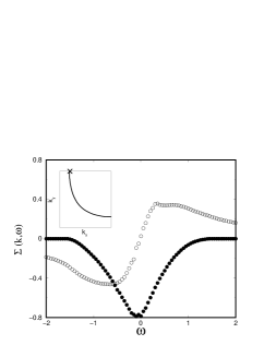
Fig.  4: The single particle self-energy ${\mit{\it\Sigma}}^{{\rm R}}(\mbox{\boldmath$k$},\omega)$ on the Fermi surface near $(0,\pi)$. The open and closed circles show the real part and the imaginary part, respectively. Here, $\mbox{\boldmath$k$}=(\pi/5,\pi)$, $g=-1.0$, $T=0.21$ and $4{\rm e}B=0.01$. The $k$-point is shown in the inset. Here, $T_{{\rm c0}}=T_{{\rm MF}}=0.196$. $T_{{\rm c0}}$ is $T_{{\rm c}}$ at $B=0$.

These features lead to the pseudogap. The corresponding one-particle spectral weight $A(\mbox{\boldmath$k$},\omega)$ and density of states $\rho(\omega)$ are shown in Fig.5. Both show the gap structure above $T_{{\rm c}}$. It should be noticed that the pseudogap is the characteristics of the strong coupling superconductivity and does not occur in the weak coupling limit. In Fig.4 and 5, we have included the magnetic field effect described in the next subsection.

Fig.  5: (a) The one-particle spectral weight $A(\mbox{\boldmath$k$},\omega)$ at $\mbox{\boldmath$k$}=(\pi/5,\pi)$. (b) The density of states $\rho(\omega)$. The open circles show the non-interacting density of states in our model, and the closed circles show the calculated result. The other parameters are the same as those in Fig.4.

The pseudogap reduces the critical temperature $T_{{\rm c}}$. The reduction becomes more remarkable as the coupling constant increases. Therefore, although the mean field critical temperature $T_{{\rm MF}}$ remarkably increases with the coupling constant $|g|$, $T_{{\rm c}}$ does not vary so much. ${}^{\hbox{\immediate{?})}}$

Here, $T_{{\rm c}}$ is scaled by the effective Fermi energy $\varepsilon_{{\rm F}}$. By considering the fact, it is naturally understood that $T_{{\rm c}}$ decreases with the doping quantity in the under-doped region. As the doping quantity decreases, the system approaches to the Mott insulator. Therefore, it should be considered that the renormalization effect for the effective Fermi energy $\varepsilon_{{\rm F}}$ is enhanced with decreasing the doping quantity. Since $T_{{\rm c}}/\varepsilon_{{\rm F}}$ is almost independent of the coupling constant $|g|$ in the strong coupling region, $T_{{\rm c}}$ decreases with $\varepsilon_{{\rm F}}$ in the under-doped region. Thus, our theory naturally and appropriately explains the pseudogap phenomena in High-$T_{{\rm c}}$ cuprates.

2.2 Magnetic field effects on the pseudogap phenomena

In this subsection, we introduce the magnetic field effect. In this paper, we consider the magnetic field applied along the c-axis, $B\parallel\vec{c}$. The main effect of the magnetic fields is the Landau level quantization for the superconducting fluctuations. It corresponds to the quantization of the orbital motion of the fluctuating Cooper pairs. The quantization is expressed by the replacement of the quadratic term of the momentum as $\mbox{\boldmath$q$}^{2}\Rightarrow 4{\rm e}B(n+\frac{1}{2})$. ${}^{\hbox{\immediate{?})}}$

The Landau quantization has the following two important effects. One is the Landau degeneracy which generally enhances the fluctuations. The Landau degeneracy reduces the dimensionality of the fluctuations. The other is the suppression of the superconductivity which weakens the pseudogap. The distance to the critical point increases as $t_{0}\Rightarrow t_{0}+2b{\rm e}B$. This corresponds to the energy level of the Lowest Landau level. When considering at the fixed temperature, the dominant effect is the latter. We can see that the characteristic magnetic field $B_{{\rm ch}}$ for the pseudogap phenomena is scaled by the quantity $t_{0}/b$, that is $B_{{\rm ch}}\propto t_{0}/b$. ${}^{\hbox{\immediate{\bf{?}})}}$ The ratio $b/t_{0}$ corresponds to the square of the GL correlation length $\xi_{{\rm GL}}$ for the superconducting fluctuations, that is, $b/t_{0}=\xi_{{\rm GL}}^{2}$. The magnetic field effects are scaled by the quantity $B\xi_{{\rm GL}}^{2}$. Thus, the pseudogap is affected by the magnetic field according to the magnetic flux penetrating the correlated area $\xi_{{\rm GL}}^{2}$.

As we mentioned above, the parameter $b$ is small in the strong coupling case. Moreover, the fact that the pseudogap phenomena take place in the wide temperature region means that $t_{0}$ is large near the pseudogap onset temperature $T^{*}$. As a result, the characteristic magnetic field $B_{{\rm ch}}$ is large, especially near $T^{*}$. In other words, the magnetic field effects are remarkably small in case of the strong coupling superconductivity. Especially, the onset temperature $T^{*}$ does not vary. Since $\xi_{{\rm GL}}$ diverges at the critical temperature $T_{{\rm c}}$, the magnetic field effects are sure to appear near $T_{{\rm c}}$. However, the region in which the effects appear is remarkably small. On the other hand, in the relatively weak coupling case, the magnetic field dependence is large and $T^{*}$ may vary. These features well explain the results of the high field NMR measurements including their doping dependence. ${}^{\hbox{\immediate{?},\penalty 1000\hskip 0.91003pt plus 0.70004pt minus 0.70004pt{?},\penalty 1000\hskip 0.91003pt plus 0.70004pt minus 0.70004pt{?},\penalty 1000\hskip 0.91003pt plus 0.70004pt minus 0.70004pt{?})}}$

Here, we have neglected the Zeeman coupling term. Although the Zeeman coupling term plays an important role at the low temperature in superconducting state, ${}^{\hbox{\immediate{\bf{?}})}}$ it has only higher order correction in the fluctuating region. This fact can be simply understood as follows. The lowest order correction of the Zeeman coupling term on the superconducting fluctuations is the second order and described as $4{\rm e}B(n+\frac{1}{2})\Rightarrow 4{\rm e}B(n+\frac{1}{2})+\frac{8}{v^{2}}(\mu B)^{2}$. Here, $v$ is a mean value of the quasi-particle velocity on the Fermi surface. $\mu=g\mu_{{\rm B}}/2$ is the magnetic moment of the electrons. Here, $g$ is the $g$-value and $\mu_{{\rm B}}$ is the Bohr magneton. Thus, the Zeeman coupling term slightly weaken the superconducting fluctuations. However, it has only higher order effect with respect to the magnetic field compared with the Landau quantization. Therefore, the effect of the Zeeman coupling term is extraordinary small in the weak coupling limit since the typical magnetic field is small. Also for High-$T_{{\rm c}}$ cuprates, it is higher order and remarkably small compared with the effect of the Landau quantization in the magnetic field of the experimentally relevant order. Actually, the magnetic field adopted in this paper is the order of ${\rm e}B\sim 10^{-2}$ in our unit. That corresponds to $B\sim 10{\rm Tesla}$. In this case, the effect of the Zeeman coupling term is higher order than that of Landau quantization as $10^{-2}$. Thus, it is justified to neglect the Zeeman coupling term. Of course, we cannot neglect the Zeeman coupling term under the extraordinary high magnetic field in the strong coupling limit. However, such an extreme situation is not realistic. When the magnetic field is applied perpendicular to the c-axis $B\perp\vec{c}$, effect of the Zeeman coupling term is relatively important because the coherence length along the c-axis $\xi_{{\rm c}}$ is small.

3 Magnetic Field Dependence of the NMR Spin-Lattice Relaxation Rate, $1/T_{1}T$

In this section, we actually calculate the NMR spin-lattice relaxation rate $1/T_{1}T$ under the magnetic field with the recent high field NMR measurements in mind. We calculate $1/T_{1}T$ by using the general expression,

$$1/T_{1}T=\sum_{\mbox{\boldmath$q$}}|A(\mbox{\boldmath$q$})|^{2}[\frac{1}{\omega}{\rm Im}\chi_{{\rm s}}^{{\rm R}}(\mbox{\boldmath$q$},\omega)\mid_{\omega\to 0}].$$ (3.1)

Here, we neglect the momentum dependence of the hyperfine coupling $A(\mbox{\boldmath$q$})$ for simplicity, which does not affect the magnetic field dependence of $1/T_{1}T$.

We calculate the spin susceptibility $\chi_{{\rm s}}^{{\rm R}}(\mbox{\boldmath$q$},\omega)$ which corresponds to the two-body correlation function shown in Fig.6.

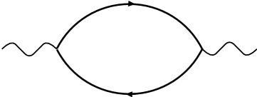
Fig.  6: The diagram representing the dynamical spin susceptibility $\chi_{{\rm s}}^{{\rm R}}(\mbox{\boldmath$q$},\omega)$

Here, the solid lines are the renormalized Green function ${\mit{\it G}}^{{\rm R}}(\mbox{\boldmath$k$},\omega)=(\omega-\varepsilon_{\mbox{\boldmath$k$}}-{\mit{\it\Sigma}}^{{\rm R}}(\mbox{\boldmath$k$},\omega))^{-1}$. The self-energy ${\mit{\it\Sigma}}^{{\rm R}}(\mbox{\boldmath$k$},\omega)$ is calculated by using the T-matrix approximation as we described before. The effects of the superconducting fluctuations are included in the self-energy.

In calculating the self-energy ${\mit{\it\Sigma}}^{{\rm R}}(\mbox{\boldmath$k$},\omega)$, we linearize the dispersion relation as $\varepsilon_{\mbox{\boldmath$k$}-\mbox{\boldmath$q$}}=\varepsilon_{\mbox{\boldmath$k$}}-\mbox{\boldmath$v$}_{\mbox{\boldmath$k$}}\mbox{\boldmath$q$}$. This linearization is justified because the only small region around $\mbox{\boldmath$q$}=0$ contributes to the self-energy. We replace the quadratic term as $\mbox{\boldmath$q$}^{2}\Rightarrow 4{\rm e}B(n+\frac{1}{2})$. This process corresponds to the Landau level quantization for the superconducting fluctuations.

From eq.(3.1), $1/T_{1}T$ is expressed as,

$$1/T_{1}T = -\sum_{\mbox{\boldmath$k$},\mbox{\boldmath$q$}}\int\frac{{\rm d}\omega}{\pi}f^{\prime}(\omega){\rm Im}{\mit{\it G}}^{{\rm R}}(\mbox{\boldmath$k$},\omega){\rm Im}{\mit{\it G}}^{{\rm R}}(\mbox{\boldmath$k+q$},\omega)$$ (3.2)

$$= -\pi\int{\rm d}\omega f^{\prime}(\omega)\rho(\omega)^{2}.$$

Here, $f^{\prime}(\omega)$ is the differential of the Fermi distribution function. This expression is reduced to the well-known expression $1/T_{1}T=\pi\rho(0)^{2}$ at $T=0$. After all, we calculate the decrease of $1/T_{1}T$ by the suppression of the density of states.

Generally speaking, we can consider the Aslamazov-Larkin term (AL term) and the Maki-Thompson term (MT term) as corrections by the fluctuations on the two-body correlation function. ${}^{\hbox{\immediate{?},\penalty 1000\hskip 0.91003pt plus 0.70004pt minus 0.70004pt{?})}}$ However, the AL term dose not exist in calculating the spin susceptibility $\chi_{{\rm s}}^{{\rm R}}(\mbox{\boldmath$q$},\omega)$. We can understand this fact by considering the spin index for the spin singlet pairing. ${}^{\hbox{\immediate{?},\penalty 1000\hskip 0.91003pt plus 0.70004pt minus 0.70004pt{?})}}$ The contribution from the MT term is small in case of the d-wave pairing, and suppressed by the slight elastic scattering. ${}^{\hbox{\immediate{?})}}$ Therefore, we have only to calculate the decrease of $1/T_{1}T$ by the pseudogap as the effect of the superconducting fluctuations.

Of course, we have to take account of the anti-ferromagnetic spin-fluctuations in order to describe the whole temperature dependence of $1/T_{1}T$. $1/T_{1}T$ increases owing to the anti-ferromagnetic spin fluctuations in the normal phase ($T>T^{*}$), and decreases owing to the superconducting fluctuations in the pseudogap phase ($T^{*}>T>T_{{\rm c}}$). Generally speaking, the magnetic field is considered to have a great effect on the superconducting fluctuations, while the effect on the spin-fluctuations is comparatively small. Because we pay attention to the magnetic field dependence in this paper, we have only to calculate the decrease of $1/T_{1}T$ due to the superconducting fluctuations and its magnetic field dependence. Actually, the misinterpretation for the experimental results is caused by the loss of the understanding of the magnetic field effect on the superconducting fluctuations in case of the strong coupling superconductivity. Our calculation gives a clear understanding about the magnetic field dependence of the pseudogap phenomena.

Even if the effect of the exchange enhancement is taken into account, the results for the magnetic field effect do not change, qualitatively. At the last of this section, we definitely calculate the effect of the exchange enhancement within the random phase approximation (RPA). Qualitatively, the same results are given there.

The calculated results are shown in Fig.7, 8 and 9. In all figures, the magnetic field is varied as $4{\rm e}B=0.01,0.02,0.05$ and $0.1$ in our unit. The horizontal axis is the temperature scaled by the zero-field critical temperature $T_{{\rm c}0}$. All results can be understood by considering the characteristic magnetic field, as we have mentioned in the previous section,

$$B_{{\rm ch}}\propto t_{0}/b=\xi_{{\rm GL}}^{-2}.$$ (3.3)

The results for the relatively weak coupling case $g=-0.5$ are shown in Fig.7. In this case, only the weak pseudogap is observed in the narrow temperature region. We consider that this case corresponds to the slightly over-doped or optimally-doped cuprates. The magnetic field dependence of $1/T_{1}T$ is clearly observed and $T^{*}$ varies. These behaviors are consistent with the NMR experiments in the slightly over-doped cuprates. ${}^{\hbox{\immediate{?})}}$

Fig.  7: The calculated results for $1/T_{1}T$ under the various magnetic field $4{\rm e}B=0.01,0.02,0.05,0.1$. The weak pseudogap case $g=-0.5$.

In case of $g=-0.8$, the magnetic field dependence is small since the parameter $b$ decreases(Fig.8). In particular, $1/T_{1}T$ is almost independent of the magnetic field near the onset temperature $T^{*}$ where the parameter $t_{0}$ is large. On the other hand, the magnetic field dependence can be observed in the vicinity of the critical temperature $T_{{\rm c}}$, since $t_{0}$ is small there.

Fig.  8: The calculated results for $1/T_{1}T$ under the magnetic field. The magnetic field is the same as that in Fig.7. The relatively strong pseudogap case $g=-0.8$.

We can see the different magnetic field dependences of the density of states according to the distance to the critical point (Fig.9). The magnetic field effect is visible in the density of states just above $T_{{\rm c}}$ (Fig.9(a)). The density of states at the low energy are recovered with increasing the magnetic field. On the other hand, the effect is almost invisible when the temperature is apart form $T_{{\rm c}}$ (Fig.9(b)).

Fig.  9: The magnetic field dependence of the density of states. Here, $g=-0.8$ and $T_{{\rm c0}}=0.1407$. The magnetic field is varied as $4{\rm e}B=0.01,0.05,0.1$. (a) in the vicinity of $T_{{\rm c}}$, $T=0.141$ (b) apart from $T_{{\rm c}}$, $T=0.15$

The results for the considerably strong coupling case $g=-1.0$ is shown in Fig.10. In this case, the strong pseudogap anomaly exists in the wide temperature region. The magnetic field effects become still smaller. The magnetic field dependence is narrowly observed in the vicinity of $T_{{\rm c}}$.

Fig.  10: The calculated results for $1/T_{1}T$ under the magnetic field. The magnetic field is the same as that in Fig.7. The strong pseudogap case $g=-1.0$.

We consider that these strong coupling cases correspond to the under-doped cuprates. These behaviors well explain the experimental results in the under-doped cuprates. ${}^{\hbox{\immediate{?})}}$ The weak effect in the vicinity of $T_{{\rm c}}$ is also observed in the experimental results. Thus, the interpretation of the experimental results as a negative evidence for the pairing scenario is inappropriate.

The strength of the superconducting coupling is indicated by the ratio $T_{{\rm c}}/\varepsilon_{{\rm F}}$. The ratio increases due to the mass renormalization by the electron-electron correlation. It should be considered that the mass-renormalization is enhanced with decreasing the doping quantity. The attractive interaction becomes strong at the same time, since the anti-ferromagnetic spin fluctuations are enhanced. Therefore, it is expected that the superconductivity becomes the strong coupling as the doping quantity decreases. Thus, the strength of the superconducting coupling naturally changes with the doping in accordance with our expectation.

It should be noticed that the change of the magnetic field effects is continuous from weak to strong coupling. In other words, the calculated results explain the NMR measurements continuously and entirely from over-doped to under-doped cuprates. Therefore, the recent high field NMR measurements including their doping dependence are regarded as an affirmative evidence for the pairing scenario.

In order to confirm the effect of the Landau degeneracy to enhance the fluctuations, we show the Fig.11. In Fig.11, the horizontal axis is scaled by the critical temperature under the magnetic field $T_{{\rm cH}}$. By keeping the distance to the critical point, we can remove the effect of the suppression of the superconductivity. Therefore, we can see the effect of the Landau degeneracy.

Fig.  11: The results for $1/T_{1}T$ in which the temperature is scaled by the critical temperature under the magnetic field $T_{{\rm cH}}$. The magnetic field is the same as that in Fig.7. Here, $g=-0.8$.

The results show that $1/T_{1}T$ decreases with increasing the magnetic field. It is because of the Landau degeneracy. The Landau degeneracy enhances the superconducting fluctuations and make the pseudogap stronger. Then, $1/T_{1}T$ is still more reduced. Therefore, even in the rather weak pseudogap case, the pseudogap may be observed clearly under the high magnetic field. In other words, the magnetic field makes the pseudogap visible in more over-doped cuprates.

At the last of this section, we consider the effect of the exchange enhancement. The exchange enhancement is taken into account within the random phase approximation (RPA). The basic results about the magnetic field effects are not changed. However, it is definitely shown that the peak of $1/T_{1}T$ ($T=T^{*}$) does not change in the strong coupling case, while the peak changes in the weak coupling case. The dynamical spin susceptibility $\chi_{{\rm RPA}}(\mbox{\boldmath$k$},\omega)$ calculated by RPA is expressed as follows.

$$\chi_{{\rm RPA}}^{{\rm R}}(\mbox{\boldmath$q$},\omega) = \frac{\chi_{0}^{{\rm R}}(\mbox{\boldmath$q$},\omega)}{1-U\chi_{0}^{{\rm R}}(\mbox{\boldmath$q$},\omega)},$$ (3.4)

$$\chi_{0}(\mbox{\boldmath$q$},{\rm i}\omega_{n}) = -T\sum_{\mbox{\boldmath$k$},\omega_{m}}{\mit{\it G}}(\mbox{\boldmath$k$},{\rm i}\omega_{m}){\mit{\it G}}(\mbox{\boldmath$k$}+\mbox{\boldmath$q$},{\rm i}\Omega_{m}+{\rm i}\omega_{n}).$$

We fix $U=1.5$ afterward. $1/T_{1}T$ is calculated by eq.(3.1). Here, we take into account the momentum dependence of the hyperfine coupling $|A(\mbox{\boldmath$q$})|^{2}=\frac{1}{2}[\{A_{1}+2B(\cos(q_{x})+\cos(q_{y}))\}^{2}+\{A_{2}+2B(\cos(q_{x})+\cos(q_{y}))\}^{2}]$. The hyperfine coupling constants $A_{1},A_{2}$ and $B$ is evaluated as $A_{1}=0.84B$ and $A_{2}=-4B$. ${}^{\hbox{\immediate{\bf{?}})}}$ The following results are not affected by the choice of the parameters, qualitatively.

The calculated results are shown in Figs.12 and 13. In the high temperature region, $1/T_{1}T$ is enhanced owing to the exchange enhancement. Near the critical temperature, $1/T_{1}T$ is reduced owing to the superconducting fluctuations. As a result, $1/T_{1}T$ shows its peak at $T=T^{*}$ above $T_{{\rm c}}$. It is a well-known pseudogap phenomenon in NMR measurements.

Fig.  12: The results for $1/T_{1}T$ including the effects of the exchange enhancement. The weak pseudogap case $g=-0.5$. the magnetic field is varied as $4{\rm e}B=0.01,0.02,$ and $0.03$ in our unit. The inset shows the results for $1/T_{2G}$

Fig.  13: The results for $1/T_{1}T$ including the effects of the exchange enhancement. The relatively strong pseudogap case $g=-0.8$. the magnetic field is varied as $4{\rm e}B=0.01,0.05,$ and $0.1$ in our unit. The inset shows the results for $1/T_{2G}$

In the weak coupling case $g=-0.5$ (Fig.12), the magnetic field effect is clearly observed. $T^{*}$ is lowered by the magnetic field. On the other hand, in the relatively strong coupling case $g=-0.8$ (Fig.13), the magnetic filed effect is remarkably small. $T^{*}$ is not changed by the magnetic field. $1/T_{1}T$ shows the magnetic filed dependence only in the vicinity of the critical temperature $T_{{\rm c}}$. These features are the same as those derived by the calculation without the effect of the exchange enhancement.

The results for the spin-echo decay rate $1/T_{2G}$ are shown in the inset of Figs.12 and 13. $1/T_{2G}$ is calculated by the following expression.

$$1/T_{2G}^{2}=\sum_{\mbox{\boldmath$q$}}[|A_{\parallel}(\mbox{\boldmath$q$})|^{2}{\rm Re}\chi_{{\rm s}}^{{\rm R}}(\mbox{\boldmath$q$},0)]^{2}-[\sum_{\mbox{\boldmath$q$}}|A_{\parallel}(\mbox{\boldmath$q$})|^{2}{\rm Re}\chi_{{\rm s}}^{{\rm R}}(\mbox{\boldmath$q$},0)]^{2}.$$ (3.6)

Here, the dynamical spin susceptibility is calculated by RPA, and $|A_{\parallel}(\mbox{\boldmath$q$})|^{2}=\{A_{2}+2B(\cos(q_{x})+\cos(q_{y}))\}^{2}$. ${}^{\hbox{\immediate{?})}}$ $1/T_{2G}$ shows the pseudogap phenomena. However, the effect of the pseudogap on $1/T_{2G}$ is weaker than that on $1/T_{1}T$. The pseudogap appears in the narrower temperature region. $1/T_{2G}$ shows its peak below the pseudogap onset temperature $T^{*}$ in $1/T_{1}T$. These results are consistent with the experimental results. ${}^{\hbox{\immediate{\bf{?}})}}$

These results indicate that the effects of the pseudogap are weak on the real part of the spin susceptibility rather than on the imaginary part at the low frequency. The dissipation (imaginary part) directly reflects the low energy density of state. However, the static property (real part) does not necessarily so. In other wards, the pseudogap suppresses the weight of the spin susceptibility at low frequency. However, the effect on the total weight is rather small. In particular, the $d$-wave pseudogap only weakly affects the real part near the anti-ferromagnetic wave vector $\mbox{\boldmath$q$}=(\pi,\pi)$. The momentum dependence of the hyperfine coupling $A_{\parallel}(\mbox{\boldmath$q$})$ still more weaken the effect of the pseudogap on $1/T_{2G}$. The above features are in common with the superconducting state. ${}^{\hbox{\immediate{\bf{?}})}}$ That is natural because the pseudogap and the superconducting gap have the same $d_{x^{2}-y^{2}}$-wave form. The magnetic field dependence of $1/T_{2G}$ has the same features as those of $1/T_{1}T$.

4 Transport in the Pseudogap Phase

In the previous sections, we have paid attention to the NMR spin-lattice relaxation rate $1/T_{1}T$ and its magnetic field dependence in the pseudogap phase. Besides that, the pseudogap affects many other measurements. These effects may be understood by considering the suppression of the one-particle spectral weight and that of the low frequency anti-ferromagnetic spin fluctuations. ${}^{\hbox{\immediate{?})}}$

In particular, the transport phenomena are enough interesting to be discussed here, because they reflect the characteristic momentum dependences of High-$T_{{\rm c}}$ cuprates and the relationship between the spin fluctuations and the superconducting fluctuations. The following qualitative discussion deserves to be described here, because there is no explicit calculation based on our understanding.

First, we describe how the transport phenomena in under-doped cuprates are understood in the normal phase ($T>T^{*}$). They are anomalous at a glance. However, we can understand them by considering the magnetic interaction caused by the anti-ferromagnetic spin fluctuations. ${}^{\hbox{\immediate{?},\penalty 1000\hskip 0.91003pt plus 0.70004pt minus 0.70004pt{\bf{?}})}}$ The momentum dependence of the lifetime of quasi-particles is important to understand the transport properties. The momentum dependent lifetime is due to the scattering by the anti-ferromagnetic spin fluctuations. ${}^{\hbox{\immediate{?},\penalty 1000\hskip 0.91003pt plus 0.70004pt minus 0.70004pt{?})}}$

’Hot spot’ means the part of the Fermi surface in which $\varepsilon_{\mbox{\boldmath$k$}}=\varepsilon_{\mbox{\boldmath$k$}+\mbox{\boldmath$Q$}}$. Here, $Q$ is a anti-ferromagnetic wave vector $\mbox{\boldmath$Q$}=(\pi,\pi)$. At ’hot spot’, quasi-particles suffer an immediate scattering by the anti-ferromagnetic spin fluctuations at $\mbox{\boldmath$q$}=\mbox{\boldmath$Q$}$. ’Cold spot’ is the area on the Fermi surface far from ’hot spot’. There, quasi-particles do not suffer the immediate scattering. Therefore, the lifetime is long at ’cold spot’ and short at ’hot spot’.

This momentum dependent lifetime is a general property of the systems with anti-ferromagnetic spin fluctuations. ${}^{\hbox{\immediate{\bf{?}})}}$ For High-$T_{{\rm c}}$ cuprates, ’hot spot’ is located near $(\pi,0)$ and its symmetric points. ’Cold spot’ is located near $(\pi/2,\pi/2)$. At the same time, the pseudogap is large at ’hot spot’ and small at ’cold spot’ because of its $d_{x^{2}-y^{2}}$-wave shape.

’Hot spot’ does not contribute to the in-plane conductivity, because the conductivity is almost determined by the most easily flowing quasiparticles. The in-plane conductivity is mainly determined by ’cold spot’. The quasiparticles at ’cold spot’ are sure to have the $T^{2}$-damping rate at the low temperature limit which is consistent with the conventional Fermi liquid theory. However, they have the $T$-linear damping rate above the relatively low crossover temperature ($T>T_{{\rm cr}}$). It is because of the low energy magnetic excitations. The transformation of the Fermi surface which leads to a form more appropriate to the nesting reduces the crossover temperature $T_{{\rm cr}}$. The transformation itself is due to the anti-ferromagnetic spin fluctuations. ${}^{\hbox{\immediate{?})}}$ As a result, the in-plane resistivity shows a $T$-linear law in the normal phase ($T>T^{*}>T_{{\rm cr}}$). It should be noticed that $T$-linear resistivity is not due to the Curie-Weiss law $\chi_{{\rm s}}(\mbox{\boldmath$Q$})\propto 1/(T+\theta)$, or $1/T_{1}T\propto 1/(T+\theta)$. The calculations inappropriately treating the momentum dependent lifetime attribute the $T$-linear resistivity to the Curie-Weiss law. ${}^{\hbox{\immediate{?},\penalty 1000\hskip 0.91003pt plus 0.70004pt minus 0.70004pt{\bf{?}})}}$ For example, the approximate relation between the in-plane resistivity $\rho_{{\rm ab}}$ and $1/T_{1}T$, $\rho_{{\rm ab}}\propto T^{2}/(T_{1}T)$ is derived. ${}^{\hbox{\immediate{?})}}$ If appropriately considering ’hot spot’ and ’cold spot’, the $T$-linear resistivity is realized more generally, but in more high temperature region. ${}^{\hbox{\immediate{?})}}$ This generality is important to understand the $T$-linear in-plane resistivity in the pseudogap phase.

The other important character of High-$T_{{\rm c}}$ cuprates is a momentum dependence of the interlayer hopping matrix element $t_{\perp}(\mbox{\boldmath$k$})$. The band calculation has shown that the dispersion along the c-axis is large at ’hot spot’ and is nearly $0$ at ’cold spot’. ${}^{\hbox{\immediate{\bf{?}})}}$ $t_{\perp}(\mbox{\boldmath$k$})$ is approximately expressed as ${}^{\hbox{\immediate{?},\penalty 1000\hskip 0.91003pt plus 0.70004pt minus 0.70004pt{\bf{?}})}}$

$$t_{\perp}(\mbox{\boldmath$k$})\propto(\frac{{\rm cos}k_{x}-{\rm cos}k_{y}}{2})^{2}.$$ (4.1)

Since the quasiparticle velocity along the c-axis is nearly $0$ at ’cold spot’, ’cold spot’ does not contribute to the c-axis conductivity. On the other hand, the contribution from ’hot spot’ is reduced by the short lifetime, in spite of the large velocity along the c-axis. As a result, the c-axis transport becomes incoherent. Thus, we can understand the coherent in-plane conductance and the incoherent c-axis conductance at the same time. ${}^{\hbox{\immediate{?})}}$

The momentum dependent lifetime enhances the Hall coefficient $R=\sigma_{xy}/\sigma_{xx}^{2}H$. ${}^{\hbox{\immediate{?})}}$ However, the vertex correction plays a more important role for the Hall coefficient. ${}^{\hbox{\immediate{?})}}$ It is because of the momentum derivative of the total current $J_{\nu}$ in the general formula given by Kohno and Yamada. ${}^{\hbox{\immediate{\bf{?}})}}$ The Hall coefficient is strongly enhanced by the vertex correction. In the conventional metals, the vertex correction gives only an constant factor arising from the Umklapp scattering and has no significant effect. ${}^{\hbox{\immediate{\bf{?}})}}$ The significance of the vertex correction is also due to the anti-ferromagnetic spin fluctuations. The vertex correction is not so important for the longitudinal conductivity even in the systems with spin fluctuations. ${}^{\hbox{\immediate{?})}}$

Here, we consider the transport phenomena in the pseudogap phase. The main effects of the pseudogap on the transport phenomena are the following two points. One is the pseudogap itself. The other is the suppression of the anti-ferromagnetic spin fluctuations.

Because of the singlet pairing correlation, the low frequency part of the anti-ferromagnetic spin fluctuations is expected to be suppressed. Indeed, NMR measurements show the suppression of $(T_{1}T)^{-1}$ and $(T_{2G})^{-1}$. ${}^{\hbox{\immediate{?},\penalty 1000\hskip 0.91003pt plus 0.70004pt minus 0.70004pt{?},\penalty 1000\hskip 0.91003pt plus 0.70004pt minus 0.70004pt{\bf{?}})}}$ The low frequency part of the anti-ferromagnetic spin fluctuations causes the quasiparticle damping. Therefore, the quasiparticle damping due to the anti-ferromagnetic spin fluctuations is immediately affected by the pseudogap.

As is shown in §2, the imaginary part of the self-energy due to the superconducting fluctuations, ${\rm Im}{\mit{\it\Sigma}}^{{\rm R}}(\mbox{\boldmath$k$},\omega)$ is remarkably large in the pseudogap phase. The large imaginary part leads to the pseudogap near $(\pi,0)$. Therefore, the contribution to the conductivity from the quasiparticles near $(\pi,0)$ is remarkably suppressed by the pseudogap itself. However, quasiparticles at ’hot spot’ do not contribute to the in-plane conductivity from the beginning. The in-plane conductivity is determined by the contribution from ’cold spot’. Therefore, the pseudogap itself is not important for the in-plane conductivity. The suppression of the anti-ferromagnetic spin fluctuations slightly reduces the scattering at ’cold spot’. Quasiparticles at ’cold spot’ are not affected by the strong scattering due to the spin fluctuations at $\mbox{\boldmath$q$}=\mbox{\boldmath$Q$}$. Therefore, the effect of the suppression of the anti-ferromagnetic spin fluctuations is small at ’cold spot’ rather than at ’hot spot’. As a result, the in-plane resistivity slightly deviates downward and keep the $T$-linear law. ${}^{\hbox{\immediate{?})}}$ This behavior is observed in many under-doped compounds and the downward deviation coincides with the pseudogap. ${}^{\hbox{\immediate{?})}}$ Thus, the $T$-linear resistivity generally appears owing to the low frequency magnetic excitations. The $T$-linear law in the pseudogap phase can not be understood by the phenomenological relation, $\rho_{{\rm ab}}\propto T^{2}\chi_{{\rm s}}(\mbox{\boldmath$Q$})$ or $\rho_{{\rm ab}}\propto T^{2}/(T_{1}T)$.

On the other hand, the pseudogap itself has more drastic effect on the c-axis conductivity. The c-axis conductance is determined by the contribution from the vicinity of $(\pi,0)$. Quasiparticles near $(\pi,0)$ decrease the contribution to the c-axis conductivity owing to the pseudogap. The pseudogap is large there. Therefore, the c-axis conductivity is remarkably suppressed by the pseudogap. This effect is confirmed within the formalism in this paper. We calculate the c-axis resistivity by using the Kubo formula and neglecting the vertex correction. The c-axis conductivity is expressed as

$$\sigma_{{\rm c}}(T)=de^{2}\sum_{\mbox{\boldmath$k$}}t_{\perp}^{2}(\mbox{\boldmath$k$})\int\frac{{\rm d}\omega}{\pi}(-f^{\prime}(\omega)){\rm Im}{\mit{\it G}}^{{\rm R}}(\mbox{\boldmath$k$},\omega){\rm Im}{\mit{\it G}}^{{\rm R}}(\mbox{\boldmath$k$},\omega).$$ (4.2)

Here, $d$ is the interlayer distance. We normalize the conductivity by the constant factor $de^{2}$. The calculated result is shown in Fig.14. The c-axis resistivity shows the semi-conductive behavior near the critical point $T_{{\rm c}}$. It is because the scattering due to the superconducting fluctuations becomes remarkable with approaching the critical temperature.

Fig.  14: The normal state c-axis resistivity $\rho_{{\rm c}}$. Here, $g=-0.8$.

Thus, we can understand the drastic increase of the c-axis resistivity in the pseudogap phase, while the in-plane resistivity changes only a little.

Because of the momentum dependence of the hopping matrix element, the c-axis transport reflects the electronic state near $(\pi,0)$. Therefore, we can see the pseudogap by observing the c-axis optical conductivity, ${}^{\hbox{\immediate{?})}}$ while the in-plane optical conductivity does not clearly indicate the pseudogap.

For the Hall conductivity, both two points play an important role. Because of the suppression of the spin fluctuations, the enhancement of the Hall coefficient due to the spin fluctuations is reduced. Moreover, since the vertex correction is large around ’hot spot’, ${}^{\hbox{\immediate{?})}}$ the pseudogap itself affects the vertex correction. The pseudogap opens at ’hot spot’ and reduces the effects of the vertex correction. Due to the two effects, the Hall coefficient is reduced and shows its peak in the pseudogap phase.

These results well explain the observed transport phenomena in the pseudogap phase. ${}^{\hbox{\immediate{?})}}$ Thus, the transport phenomena in the pseudogap phase is naturally understood by considering the $d_{x^{2}-y^{2}}$-wave pseudogap.

5 Summary and Discussion

In this paper, we have shown that the pairing scenario based on the strong coupling superconductivity well explains the effects of the magnetic field on the pseudogap phenomena in High-$T_{{\rm c}}$ cuprates.

We have shown in the previous paper ${}^{\hbox{\immediate{?})}}$ that the pseudogap phenomena are properly described as a precursor of the superconductivity under the reasonable conditions. In this paper, we have used the same formalism for calculating the single-particle self-energy and introduce the magnetic field effects thorough the Landau level quantization. We explicitly calculated the NMR spin-lattice relaxation rate $1/T_{1}T$ to compare the obtained results with the results of the recent high field NMR measurements.

The dominant effect of the Landau quantization is the suppression of the superconductivity, while the Landau degeneracy itself enhances the superconducting fluctuations. From the simple discussion, we can see that the characteristic magnetic field is scaled as $B_{{\rm ch}}\propto t_{0}/b=\xi_{{\rm GL}}^{-2}$. Actually, the calculated results support this behavior. In the relatively weak coupling case, the weak pseudogap is observed in the narrow temperature region. Then, the characteristic magnetic field is small and the magnetic field effects are visible. On the other hand, in the strong coupling case where the pseudogap is observed in the wide temperature region, the characteristic magnetic field is large. In particular, it is remarkably large near the onset temperature $T^{*}$. Therefore $T^{*}$ is almost independent of the magnetic field. The magnetic field effects are visible only in the vicinity of the critical temperature $T_{{\rm c}}$. It should be noticed that the characteristic magnetic field $B_{{\rm ch}}$ near $T^{*}$ is different from that near $T_{{\rm c}}$. When the pseudogap phenomena take place at $T^{*}$, the superconducting correlation length $\xi_{{\rm GL}}$ is still short. Therefore, the pseudogap is not so affected by the magnetic field near $T^{*}$.

By considering that the effective Fermi energy $\varepsilon_{{\rm F}}$ decreases and the attractive interaction increases with decreasing the doping quantity, the calculated results well explain the high field NMR measurements including their doping dependence. The explanation is continuous from over-doped to under-doped cuprates.

There is an interpretation that the magnetic field independence of the pseudogap phenomena in under-doped cuprates is an evidence denying the pairing scenarios for the pseudogap. ${}^{\hbox{\immediate{?})}}$ However, the pairing scenario based on the strong coupling superconductivity naturally explains the experiments including their doping dependence.

Moreover, the continuous understanding in the phase diagram rather support the pairing scenario. In the pseudogap phase, the self-energy correction due to the superconducting fluctuations is a common mechanism in reducing the density of states and $1/T_{1}T$. Because the pseudogap phenomena continuously take place from slightly over-doped to under-doped cuprates, their magnetic field dependences should be continuously understood. The pseudogap becomes strong as the doping quantity decreases. The magnetic field dependence of the weak pseudogap case can be understood within the conventional weak coupling theory for the superconducting fluctuations. ${}^{\hbox{\immediate{?},\penalty 1000\hskip 0.91003pt plus 0.70004pt minus 0.70004pt{?})}}$ Our theory is an extension of the theory. This fact indicates the correctness of our description for the pseudogap phenomena in under-doped cuprates based on the strong coupling superconductivity.

On the other hand, it is not clear whether the magnetic origin may be consistent with the magnetic field dependence, especially in the weak pseudogap case. It is because the magnetic exchange coupling $J$ is the order of $J\sim 1000{\rm K}$ and the applied magnetic field is the order of $\mu_{{\rm B}}B\sim 10{\rm K}$.

Moreover, we have discussed the transport phenomena in the pseudogap phase. Generally speaking, the transport phenomena in the normal phase are explained by the effects of the anti-ferromagnetic spin fluctuations. We have shown that the transport coefficients in the pseudogap phase are naturally understood by considering the characteristic momentum dependences of both the spin- and the superconducting fluctuations in addition to the momentum dependence of the c-axis transfer matrix. The c-axis conductivity is mainly determined by the region near $(\pi,0)$. Therefore, the c-axis transport directly reflects the pseudogap. We have definitely shown the remarkable increase of the c-axis resistivity in the pseudogap phase.

Here, we give a brief discussion on the self-consistent calculation. In the self-consistent calculation the pseudogap is described in a similar way. The fundamental picture does not change also in the self-consistent calculation, although the renormalization effects on the TDGL parameters exist. However, the self-consistent T-matrix calculation is one of the methods introducing the criticality of the superconducting fluctuations. This effect corresponds to the forth order term in the Ginzburg-Landau description. The forth order term in the Ginzburg-Landau action is expressed by the diagram shown in Fig.15. This term indicates the repulsive interaction between the fluctuating Cooper pairs (that is the mode coupling term).

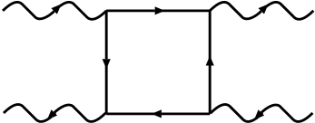
Fig.  15: The diagram representing the repulsive interaction between the fluctuating Cooper pairs. The wavy and solid lines represent the propagator of the fluctuating Cooper pairs and that of the fermions, respectively.

The effect of this term is included in the self-consistent calculation at least in the level of the Hartree-Fock approximation. Thus, the criticality of the superconducting fluctuations is introduced. The criticality makes the magnetic field dependence still smaller. To put it in detail, in the self-consistent calculation, $t_{0}$ depends on the magnetic field. As the magnetic field suppresses the pseudogap, $t_{0}(B)$ is reduced. Therefore, the distance to the superconductivity $t_{0}(B)+2b{\rm e}B$ varies more slowly than $t_{0}(0)+2b{\rm e}B$. Thus, the magnetic field dependence is reduced by the criticality. Anyway, the strong coupling superconductivity is the essential factor for the magnetic field independence, as we described in this paper. The existence of the wide critical region is a result of the strong coupling superconductivity.

The more systematic measurements of the magnetic field dependences in the various doping rate will be an important verification to determine the origin of the pseudogap in High-$T_{{\rm c}}$ cuprates.

References

- [1] J. G. Bednortz and K. A. Mller: Z. Phys. B 64 (1986) 189.
- [2] W. W. Warren, R. E. Walstedt, G. F. Brennert, R. J. Cava, R. Tycko, R. F. Bell and G. Dabbagh: Phys. Rev. Lett. 62 (1989) 1193; M. Takigawa, A. P. Reyes, P. C. Hammel, J. D. Thompson, R. H. Heffner, Z. Fisk and K. C. Ott: Phys. Rev. B 43 (1991) 247; M. H. Julien, P. Carretta, M. Horvati: Phys. Rev. Lett. 76 (1996) 4238; H. Yasuoka, S. Kambe, Y. Itoh and T. Machi: Physica. B 199&200 (1994) 278; K. Ishida, K. Yoshida, T. Mito, Y. Tokunaga, Y. Kitaoka, K. Asayama, Y. Nakayama, J. Shimoyama and K. Kishio: Phys. Rev. B 58 (1998) R5960.
- [3] C. C. Homes, T. Timusk, R. Liang, D. A. Bonn and W. H. Hardy : Phys. Rev. Lett. 71 (1993) 1645; D. N. Basov, R. Liang, B. Dabrowski, D. A. Bonn, W. N. Hardy and T. Timusk: Phys. Rev. Lett. 77 (1996) 4090.
- [4] For example, T. Ito, K. Takenaka and S. Uchida: Phys. Rev. Lett. 70 (1993) 3995; K. Mizuhashi, K. Takenaka, Y. Fukuzumi and S. Uchida: Phys. Rev. B 52 (1995) R3884; M. Oda, K. Hoya, R. Kubota, C. Manabe, N. Momono, T. Nakano and M. Ido: Physica. C 281 (1997) 135.
- [5] H. Ding, T. Yokoya, J. C. Campuzano, T. Takahashi, M. Randeria, M. R. Norman, T. Mochiku, K. Kadowaki and J. Giapintzakis: Nature. 382 (1996) 51; A. G. Loeser, Z. X. Shen, D. S. Dessau, D. S. Marshall, C. H. Park, P. Fournier and A. Kapitulnik: Science. 273 325.
- [6] Ch. Renner, B. Revaz, J.-Y. Genoud, K. Kadowaki and Ø. Fischer: Phys. Rev. Lett. 80 (1998) 149.
- [7] N. Momono, T. Matsuzaki, T. Nagata, M. Oda and M. Ido: to be published in J. Low. Temp. Phys.
- [8] Y. Yanase and K. Yamada: J. Phys. Soc. Jpn 68 (1999) 2999.
- [9] M. R. Norman, H. Ding, M. Randeria, J. C. Campuzano, T. Yokoya, T. Takeuchi, T. Takahashi, T. Mochiku, K. Kadowaki, P. Guptasarma and D. G. Hinks: Nature. 392 (1998) 157.
- [10] T. Tanamoto, H. Kohno and H. Fukuyama: J. Phys. Soc. Jpn 63 (1994) 2739.
- [11] A. Kampf and J. R. Schrieffer: Phys. Rev. B 41 (1990) 6399; A. V. Chubukov, D. K. Morr and K. A. Shakhnovich: Philos. Mag. B 74 (1996) 563; D. Pines: Z. Phys. B 103 (1997) 129; A. V. Chubukov and J. Schmalian: Phys. Rev. B 57 (1998) 11085.
- [12] V. J. Emery and S. A. Kivelson: Phys. Rev. Lett. 74 (1995) 3253.
- [13] M. Franz and A. J. Millis: Phys. Rev. B 58 (1998) 14572; H. J. Kwon and A. T. Dorsey: Phys. Rev. B 59 (1999) 6438.
- [14] M. Randeria: preprint. (cond-mat/9710223); C. A. R. S de Melo, M. Randeria and J. R. Engelbrecht: Phys. Rev. Lett. 71 (1993) 3202.
- [15] P. Nozires and S. Schmitt-Rink: J. Low Temp. Phys. 59 (1985) 195; A. J. Leggett: Modern Trends in the Theory of Condensed Matter ed. A. Pekalski and R. Przystawa (Springer-Verlag, Berlin, 1980).
- [16] O. Tchernyshyov: Phys. Rev. B 56 (1997) 3372.
- [17] B. Jank, J. Maly and K. Levin: Phys. Rev. B 56 (1997) 11407; J. Maly, B. Jank and K. Levin: preprint. (cond-mat/9805018)
- [18] G-q. Zheng, W. G. Clark, Y. Kitaoka, K. Asayama, K. Kodama, P. Kuhns and W. G. Moulton: Phys. Rev. B 60 (1999) R9947.
- [19] K. Gorny, O. M. Vyaselev, J. A. Martindale, V. A. Nandor, C. H. Pennington, P. C. Hammel, W. L. Hults, J. L. Smith, P. L. Kuhns, A. P. Reyes and W. G. Moulton: Phys. Rev. Lett. 82 (1999) 177.
- [20] V. F. Mitrovi, H. N. Bachman, W. P. Halperin, M. Eschrig, J. A. Sauls, A. P. Reyes, P. Kuhns and W. G. Moulton: Phys. Rev. Lett. 82 (1999) 2784; V. F. Mitrovi, H. N. Bachman, W. P. Halperin, M. Eschrig and J. A. Sauls: preprint. (cond-mat/9901232)
- [21] G-q. Zheng: private communication.
- [22] M. Eschrig, D. Rainer and J. A. Sauls: Phys. Rev. B 59 (1999) 12095.
- [23] P. Monthoux, A. V. Balatsky and D. Pines: Phys. Rev. B 46 (1992) 14803.
- [24] T. Moriya, Y. Takahashi and K. Ueda: J. Phys. Soc. Jpn 59 (1990) 2905.
- [25] B. P. Stojkovi and D. Pines: Phys. Rev. Lett. 76 (1996) 811; B. P. Stojkovi and D. Pines: Phys. Rev. B 55 (1997) 8576.
- [26] Y. Yanase and K. Yamada: J. Phys. Soc. Jpn 68 (1999) 548.
- [27] T. Dahm, D. Manske and L. Tewordt: Phys. Rev. B 55 (1997) 15274.
- [28] S. Koikegami and K. Yamada: to be published in J. Phys. Soc. Jpn.
- [29] L. G. Aslamazov and A. I. Larkin: Fiz. Tverd. Tela. 10 (1968) 1104. [Sov. Phys. Solid State 10 (1968) 875.]
- [30] K. Maki: Prog. Theor. Phys 40 (1968) 193.; R. S. Thompson: Phys. Rev. B 1 (1970) 327.
- [31] K. Kuboki and H. Fukuyama: J. Phys. Soc. Jpn 58 (1989) 376; J. Heym: J. Low Temp. Phys. 89 (1992) 869; M. Randeria and A. A. Varlamov: Phys. Rev. B 50 (1994) 10401; C. Di Castro, R. Raimondi, C. Castellani and A. A. Varlamov: Phys. Rev. B 42 (1990) 10221; A. A. Varlamov, G. Balestrino, E. Milani and D. V. Livanov: Adv. Phys. 48 (1999) 655.
- [32] H. Ebisawa and H. Fukuyama: Prog. Theor. Phys 46 (1971) 1042.
- [33] Y. Yanase and K. Yamada: to be published in Physica. B (2000).
- [34] P. Fulde and R. A. Ferrell: Phys. Rev. 135 (1964) A550; A. I. Larkin and Y. N. Ovchinnikov: Sov. Phys. -JETP 20 (1965) 762.
- [35] V. Barzykin and D. Pines: Phys. Rev. B 52 (1995) 13585.
- [36] Y. Tokunaga et al.: to be published in Physica. B (2000).
- [37] N. Bulut and D. J. Scalapino: Phys. Rev. Lett. 67 (1991) 2898.
- [38] H. Kontani, K. Kanki and K. Ueda: Phys. Rev. B 59 (1999) 14723; K. Kanki and H. Kontani: J. Phys. Soc. Jpn 58 (1999) 1614.
- [39] A. Rosch: Phys. Rev. Lett. 82 (1999) 4280; A. Rosch: preprint. (cond-mat/9908245)
- [40] H. Kohno and K. Yamada: Prog. Theor. Phys. 85 (1991) 13.
- [41] O. K. Anderson, A. I. Liechtenstein, O. Jepsen and F. Paulsen: J. Phys. Chem. Solids. 56 (1995) 1573.
- [42] L. B. Ioffe and A. J. Millis: Phys. Rev. B 58 (1998) 11631.
- [43] H. Kohno and K. Yamada: Prog. Theor. Phys. 80 (1988) 623.
- [44] K. Yamada and K. Yosida: Prog. Theor. Phys. 76 (1986) 621.
- [45] Y. Itoh, T. Machi, S. Adachi, A. Fukuoka, K. Tanabe and H. Yasuoka: J. Phys. Soc. Jpn. 67 (1998) 312.