$1/f^{\alpha}$ fluctuations in a ricepile model

Abstract

The temporal fluctuation of the average slope of a ricepile model is investigated. It is found that the power spectrum $S(f)$ scales as $1/f^{\alpha}$ with $\alpha\approx 1.3$ when grains of rice are added only to one end of the pile. If grains are randomly added to the pile, the power spectrum exhibits $1/f^{2}$ behavior. The profile fluctuations of the pile under different driving mechanisms are also discussed.

PACS numbers: 05.40.-a, 05.65.+b, 45.70.-n, 05.70.Ln

The term flick noise refers to the phenomenon that a signal $s(t)$ fluctuates with a power spectrum $S(f)\propto 1/f^{\alpha}$ at low frequency. Since the exponent $\alpha$ is often close to $1$, flick noise is also called $1/f$ noise. The power spectrum of a signal is defined as the Fourier transform of its auto-correlation function $C(t_{0},t)=\langle s(t_{0})s(t)\rangle$, where $\langle\cdots\rangle$ denotes ensemble average. Usually the signal $s(t)$ under study is stationary and its auto-correlation function only depends on $t-t_{0}$. The auto-correlation function can be alternatively calculated as

$$C(\tau)=\int_{-\infty}^{\infty}s(t)s(t+\tau)dt.$$ (1)

If the signal is real-valued, its power spectrum is just

$$S(f)=\left|\widehat{s}(f)\right|^{2}$$ (2)

according to Wiener-Khinchin Theorem. Here $\widehat{s}(f)$ is the Fourier transform of the signal

$$\widehat{s}(f)=\int_{-\infty}^{\infty}s(t)e^{i2\pi ft}dt.$$ (3)

In nature and laboratory, many physical systems show flick noise. For example, flick noise appears in a variety of systems ranging from the light of quasars [1] to water flows in rivers [2], music and speech [3], and electrical measurement [4, 5]. Despite its ubiquity, a universal explanation of the flick noise is still lacking. Bak, Tang, and Wiesenfeld have proposed that self-organized criticality (SOC) [6] may be the mechanism underlying flick noise. They also demonstrated their idea of SOC with a cellular automaton model, the BTW sandpile model. However, the model they proposed does not exhibit flick noise in its 1D and 2D versions [7]. Especially the 1D BTW sandpile model does not even exhibit SOC behavior. Experiments [8] on piles of rice grains were done to investigate if real granular systems display SOC behaviors. It was found that ricepiles with elongated rice grains exhibit SOC behaviors. The key ingredient here is the heterogeneity of the system. Because elongated rice grains could be packed in different ways [8], the ricepile thus has many different metastable states. A 1D model of ricepile was proposed by the same group of authors; avalanche distribution and transit-time distributions were discussed [9]. The model was later investigated by several other authors including us [10, 11, 12]. Attentions were paid to the avalanche dynamics and transit-time statistics of the model. In this paper, we are concerned with temporal fluctuation of the average slope of the system. We want to investigate if it has flick noise or flick-like behavior.

The ricepile model is defined as follows: Consider a one-dimensional array of sites $1$, $2$, $\cdots$, $L$. Each site contains an integer number $h_{i}$ of rice grains. Here $h_{i}$ is called the local height of the ricepile at site $i$. The system is initialized by setting $h_{i}=0$ for all sites. This means the ricepile is to be built up from scratch. The system is driven by dropping rice grains onto the pile. If one grain of rice is dropped at site $i$, then the height of column $i$ will increase by $1$, $h_{i}\rightarrow h_{i}+1$. With the dropping of rice grains, a ricepile is built up. The local slope of the pile is defined as $z_{i}=h_{i}-h_{i+1}$. Whenever the local slope $z_{i}$ exceeds certain threshold $z_{i}^{c}$ (specified in the following), site $i$ will topple and one grain of rice will be transferred to its neighbor site on the right. That is, $h_{i}\rightarrow h_{i}-1$ and $h_{i+1}\rightarrow h_{i+1}+1$. In this model, rice grains are allowed to leave the pile only from the right end of the pile, while the left end of the pile is closed. So the boundary condition is kept as $h_{0}=h_{1}$ and $h_{L+1}=0$. The ricepile is said to be stable if no local slope exceeds threshold value, that is, $z_{i}\leq z_{i}^{c}$ for all $i$. Rice grains are dropped to the pile only when the pile is stable. In an unstable state, all sites $i$ with $z_{i}>z_{i}^{c}$ topple in parallel. The topplings of one or more sites is called an avalanche event, and the size of an avalanche is defined as the number of topplings involved in the avalanche event.

The values of $z_{i}^{c}$’s are essential to the definition of the model. As in Ref. [10], every time site $i$ topples, the threshold slope $z_{i}^{c}$ will take a new value randomly chosen from $1$ to $r$ with equal probability. Here $r$ is an integer no less than $1$. The parameter $r$ reflects the level of medium disorder. The larger the $r$, the higher the level of medium disorder of the system. If $r=1$ the model becomes the $1$D BTW sandpile model. When $r=2$, the model reduces to the model studied in reference [9]. In ref. [10], we have investigated the effect of disorder on the universality of the avalanche size distribution and transit time distribution.

In the present work, we performed extensive numerical simulations on the system evolution. Let us first study the case where rice grains are added only to the left end of the pile, i.e., only to the site $i=1$, which is in accordance with the experiment setup [8]. We shall refer to this driving mechanism as the fixed driving. When the stationary state is reached, we record the average slope $z(t)=h_{1}(t)/L$ of the pile after every avalanche. Here time $t$ is measured in the number of grained added to the system. Thus we got a time series $z(t)$. Typical results about the fluctuation of the slope $z(t)$ can be seen in Fig.1.a. We calculate the power spectrum of this time series according to Eq.(2). We find that for not too small systems the slope fluctuation displays $1/f$-like behavior. In fact, we got a power spectrum $S(f)$ scaling as $1/f^{\alpha}$ at low frequency, with the exponent $\alpha=1.3\pm 0.1$.

We note the following points:

(a) the temporal behavior of the ricepile model is dramatically different from the 1D BTW sandpile model. In the 1D BTW model, the system has a stable state [6], which, once reached, cannot be altered by subsequent droppings of sand grains. Thus the 1D BTW model does not display SOC behaviors. The slope of the 1D sandpile model assumes constant values. The power spectrum is thus of the form $S(f)=\delta(f)$. In words, there is only dc component in the power spectrum for the 1D BTW model.

(b) With the introduction of varying threshold $z_{i}^{c}$ into the ricepile model the behavior of the system becomes much more rich. The avalanche distribution follows power law [10], which is an important signature of SOC. Besides that, the temporal fluctuation of $z(t)$ has a power spectrum of flick type at low frequency.

We notice that the power spectrum is flattened at low frequency for small system. This is a size effect. It is believed that flick noise fluctuation is closely related to the long range spatial correlation in the system. For small system, the spatial correlation that can be built up is limited by the system size, thus the long range temporal correlation required by flick noise is truncated off at low frequency. Our numerical results verified the above discussion. In Fig. 2, we show the power spectrum of $z(t)$ for different system sizes. It is clear that when the system size increases the $1/f^{\alpha}$ behaviors extends to lower and lower frequency.

We also investigated the effect of the level of disorder on the power spectrum. This was done by simulating the system with different values of $r$. In Fig. 3 we show the power spectra for the system with different $r$. It can be seen from this figure, that the power-law (straight in the log-log plot) part extends to lower frequency for higher value of $r$. The effect can be understood by the following discussion. When the level of disorder is increased, the amplitude of the slope fluctuation also increases. Larger amplitude fluctuation of $z(t)$ requires more grains to be added to the system. Hence the period of this fluctuation increase, which gives rise to the increase of low frequency components in the power spectrum. We have made statistics on deviation of the ricepile slope from its average value in the stationary state. We found that the greater the $r$, the greater the deviation. Note that the value of $r>1$ does not affect the exponent $\alpha$, as it does not alter the universal avalanche exponent $\tau$ for the avalanche distribution [10].

It is also interesting to study the effect of driving mechanism on the temporal behavior of the system. Now, instead of dropping rice grains to the left end of the pile, we drop rice grains to randomly chosen sites of the system. This way of dropping rice grains represents a different driving mechanism, which we shall refer to as the random driving. Numerical simulations with this random driving were made and the time series $z(t)$ was recorded. For this way of driving, typical result about the fluctuation of $z(t)$ can be seen in Fig. 1.b. It seems that $z(t)$ now fluctuates more regularly than it does for the fixed driving. We found that under random driving the temporal fluctuation has a trivial $1/f^{2}$ behavior as in the case of various previously studied sandpiles [7]. In Fig. 3, we compare the power spectra of the two cases with different driving mechanisms. Two groups of curves are shown in this figure, each with a different exponent $\alpha$. For the fixed driving, we have $\alpha\approx 1.25$, while for the random driving we have $\alpha\approx 2.0$. The distinction of the two behaviors is quite clear. This shows that the driving mechanism, as an integrated part of the model, has an important role in the temporal behaviors of the system. Recent work on the continuous version of BTW sandpile model[13], and that on quasi-1D BTW model[14] also showed that certain driving mechanisms are necessary conditions for these models to display $1/f$ fluctuation for the total amount of sand (or say, energy).

Here we present an heuristic discussion on why the exponent $\alpha$ is smaller for fixed driving than for random driving. For fixed driving, the height $h_{1}$ at site $i=1$ changes almost every dropping, and so is the average slope $z(t)$. Thus the high frequency component of the $z(t)$ fluctuation has a heavier weight in its power spectrum, and this will make the exponent $\alpha$ smaller. While for the random driving, the rice grains are dropped to the pile at random sites, the spatial correlations previously built up can be easily destroyed, making the $z(t)$ behave more or less as an random walk. So the exponent $\alpha$ for this case shall be very close to $2$. For random driving, each site has the same probability in receiving a grain in every drop. For the fixed driving, however, only the left end site receive grains, so there is in some sense breaking of symmetry, which would lead to different scalings in the slope fluctuations.

To see more about the effect of driving mechanism, it is helpful to investigate the profile fluctuations of the pile under different drivings. Because avalanches change the surface of the ricepile, the pile fluctuates around an average profile, and the size of the fluctuations characterize the active zone of the ricepile surface. Let the standard deviation of height at site $i$ be $\sigma_{h}(i,L)=\sqrt{\langle h_{i}^{2}\rangle-\langle h_{i}\rangle^{2}}$. Here $\langle\cdots\rangle$ represents average over time. Then we calculate the profile width of the ricepile, $w={1\over L}\sum_{i}\sigma_{h}(i,L)$, which is a function of the system size. In Fig. 4, we show the profile width of the ricepile for different $r$ and different driving mechanisms. It can be seen that $w$ scales with $L$ as $w\propto L^{\chi}$, and that $\chi=0.25\pm 0.01$ for fixed driving, $\chi=0.09\pm 0.01$ for random driving. For given driving mechanism, $w$ increases with increasing $r$. As we stated in Ref. [10], the parameter $r$ reflects the level of medium disorder in the rice pile. Although the level of disorder does not change the scaling exponent $\chi$, it does affect the amplitude of fluctuations. For greater $r$, the profile width is larger. It can be seen in the figure, that the data points for $r=4$ are above that for $r=2$, for given driving mechanism. A recent experiment showed that piles of polished rice grains has a smaller profile width than unpolished ones[15], which have higher level of medium disorder.

In conclusion, we have studied the temporal fluctuation of the slope of ricepile model in its critical stationary state. The power spectrum of this fluctuation is closely related to the driving mechanism. When the rice grains are dropped to the left end of the pile, the slope fluctuates with a flick-type power spectrum, with the exponent $\alpha=1.3\pm 0.1$. When the driving mechanism is changed to random driving, the model displays $1/f^{2}$ behaviors. Greater system size and higher level of disorder will extend the frequency range where the power spectrum has the form $1/f^{\alpha}$.

The author thanks Prof. Vespignani for helpful discussions. This work was supported by the National Natural Science Foundation of China under Grant No. 19705002, and the Research Fund for the Doctoral Program of Higher Education (RFDP).

FIG. 1.: The time evolution of the average slope $z(t)$ of the ricepile after the stationary state has been reached. The parameters used for this figure are $L=20$, $r=4$. (a) rice grains are added to the pile at site $i=1$. (b) rice grains are added randomly to the pile.

FIG. 2.: The power spectrum of $z(t)$ for different system sizes, with fixed driving and $r=2$. The curves (from top to bottom) are for $L=40$, $60$, and $100$ respectively. The dashed line is a curve for $y\propto x^{-1.25}$ for reference. The number of data points for Fourier transformation is $N=2048$, and the results are obtained by averaging over $500$ samples. $f_{c}\equiv 1/(2\Delta)$ is the Nyquist critical frequency, where $\Delta$ is the time interval between two successive points in the Fourier transformation.

FIG. 3.: The power spectrum of the slope fluctuation for a ricepile with $L=100$. Two groups of curves are shown in this figure, with different exponents $\alpha$. For reference, the upper dashed line is a curve for $y\propto x^{-1.25}$, while the lower dotted line shows a curve $y\propto x^{-2}$. In each group of curves, the upper curve is for the case $r=4$, and the lower one is for $r=2$.

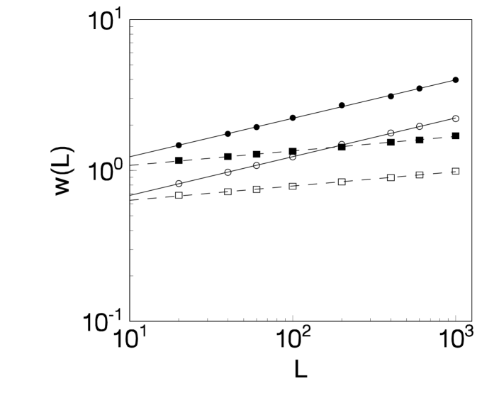
FIG. 4.: The profile width of the ricepile scales with the system size. Data from numerical simulations are shown in open (for $r=2$) or filled ( for $r=4$) symbols. Solid lines are power law fit to the data for fixed driving, with power law exponent $\chi=0.25\pm 0.01$, and the dashed lines are for random driving, with $\chi=0.09\pm 0.01$. For every run of numerical simulation, statistics were made over at least $10^{5}$ grain dropping.

REFERENCES

- [1] W. H. Press, Comments Astrophys. 7, 103(1978).
- [2] B. B. Mandelbrot and J. R. Wallis, Water Resour. Res. 4, 909 (1968); 5, 321 (1969).
- [3] R. F. Voss and J. Clarke, Nature 258, 317 (1975); J. Acoust. Soc. Am. 63, 258 (1978).
- [4] P. Dutta and P. M. Horn, Rev. Mod. Phys. 53, 497 (1981).
- [5] M. B. Weissman, Rev. Mod. Phys. 60, 537 (1988).
- [6] P. Bak, C. Tang, and K. Wiesenfeld, Phys. Rev. Lett. 59, 381 (1987); Phys. Rev. A 38, 364 (1988).
- [7] H. J. Jensen, K. Christensen, H. C. Fogedby, Phys. Rev. B 40, 7425 (1989).
- [8] V. Frette, K. Christensen, A. Malthe-Sorenssen, J. Feder, T. Jossang, and P. Meakin, Nature(London)379, 49 (1996).
- [9] K. Christensen,A. Corral, V. Frette, J. Feder and T. Jossang, Phys. Rev. Lett. 77, 107 (1996).
- [10] Shu-dong Zhang, Phys. Lett. A 233, 317 (1997).
- [11] M. Bengrine, A. Benyoussef, F. Mhirech, and S. D. Zhang, Physica A 272, 1 (1999).
- [12] L. A. N. Amaral, and K. B. Lauritsen, Phys. Rev. E 56, 231 (1997); Physica A 231, 608(1996).
- [13] P. De Los Rios and Y. -C. Zhang, Phys. Rev. Lett. 82, 472, (1999).
- [14] S. Maslov, C. Tang, and Y. -C. Zhang, Phys. Rev. Lett. 83, 2449, (1999).
- [15] A. Malthe-Sorenssen, J. Feder, K. Christensen, V. Frette, T. Jossang, Phys. Rev. Lett. 83, 764 (1999).