Fluctuations in mixtures of lamellar- and nonlamellar-forming lipids

Abstract

We consider the role of nonlamellar-forming lipids in biological membranes by examining fluctuations, within the random phase approximation, of a model mixture of two lipids, one of which forms lamellar phases while the other forms inverted hexagonal phases. To determine the extent to which nonlamellar-forming lipids facilitiate the formation of nonlamellar structures in lipid mixtures, we examine the fluctuation modes and various correlation functions in the lamellar phase of the mixture. To highlight the role fluctuations can play, we focus on the lamellar phase near its limit of stability. Our results indicate that in the initial stages of the transition, undulations appear in the lamellae occupied by the tails, and that the nonlamellar-forming lipid dominates these undulations. The lamellae occupied by the head groups pinch off to make the tubes of the hexagonal phase. Examination of different correlations and susceptibilities makes quantitative the dominant role of the nonlamellar-forming lipids.

I Introduction

It is well known that the biological, lipid bilayer membrane contains a mixture of lipids some of which, alone in aqueous solution, do not form bilayers at all. This presents the interesting question as to what possible function in the membrane these lipids can be serving[1, 2, 3]. There are two lines of thought on the answer. The first is that the nonlamellar-forming lipids, roughly characterized as having a small head group and long, splayed tails, can with these tails increase significantly the local lateral pressure distribution in the interior of the bilayer. This increased pressure may be necessary for a protein or peptide to function[4, 5, 6]. The second is that the nonlamellar-forming lipids can make less expensive the energetic cost to form a small, nonlamellar region which may be needed in processes such as membrane fusion[7, 8]. Experiment shows that there is the expected correlation between the presence of nonlamellar-forming lipids and the ability of the lamellar phase to make a transition to a nonlamellar, inverted-hexagonal one[9, 10]. There is also a correlation between the concentration of such lipids and the ability to make other nonlamellar structures, such as occur in membrane fusion[11].

In an attempt to shed some light on the role in membranes of nonlamellar-forming lipids, we first introduced[12] a relatively simple and tractable model of a lipid. We showed that it exhibited the polymorphism observed in experiment as a function of a single architectural parameter, the fraction of the total lipid volume occupied by the head group. We also showed that the phase diagram of a model aqueous lipid whose head group fraction was similar to that of dioleoylphosphatidylethanolamine was in good agreement with the measured diagram[13, 14]. We then considered a mixture of two lipids with the same headgroup but different tail length[15]. Thus they were distinguished by the different relative volume fractions of their headgroups such that one formed lamellar, $L_{\alpha}$, phases while the other formed inverted-hexagonal, $H_{II}$, ones. We examined the density profiles of the tail segments from the two different lipids in each of the two phases. In particular we determined that, in the $H_{II}$ phase of the mixture, the density of the tail segments of the nonlamellar-forming lipid varied around the Brillouin zone, with its density being largest in the direction between next-nearest-neighbor cores, as expected[16]. We were able to make quantitative this expected variation, and found the relative difference in tail segment densities to be on the order of a few percent.

The calculations in Ref. [12] and [15] were carried out within self-consistent field theory, (SCFT), and therefore ignored fluctuations. In this paper, we consider the effect of Gaussian fluctuations about the SCFT solution. This enables us to determine the effect of fluctuations, within Gaussian order, on the transition from the $L_{\alpha}$ to the $H_{II}$ phase, and to observe the initial stages of the path between them. In order to highlight the effect of fluctuations, we examine the metastable lamellar phase near its spinodal in a region of the phase diagram in which the $H_{II}$ phase is the stable one. We find that undulations occur in the lamellae occupied by the tails, and that the lamellae occupied by the head groups pinch off to form the tubes of the $H_{II}$ phase. This is similar to scenarios proposed earlier by Hui et al.[17] and Caffrey[18] and which arose from their experimental observations. The hexagonal phase that is initiated by the lowest energy fluctuation mode is characterized by a lattice parameter which is within 1% of the stable $H_{II}$ phase, and has the same orientation: one in which the tubes are coplanar with the lamellae from which they were formed. This coplanarity is in agreement with experiment[19]. We observe that the nonlamellar-forming lipids dominate the undulations in the tail region, while the lamellar-forming lipids tend to fill in the regions between the cylinders as they pinch off. To make quantitative the effect of the nonlamellar-forming lipids, we examine three different measures of their role in the transition; the correlation between the density fluctuation and the order parameter, the ratio of the susceptibilities of the two different lipids to fluctuations at the critical wavevector, and the overlap of the order parameter fluctuations of each lipid with the equilibrium $H_{II}$ structure. All these measures show the nonlamellar-forming lipids to play a significant role in bringing about the transition.

Having calculated the fluctuations in Gaussian approximation, we are able to calculate all structure factors. We show here the order parameter-order parameter structure factor, which is the one most readily measured, as well as the density-density structure factor of either lipid.

In the next section we review the theory of Gaussian fluctuations about an ordered phase[20, 21, 22] and extend it to our model of lipid mixtures. Results are presented next, and we conclude with a brief summary.

II Theory

We consider an anhydrous mixture of $n_{1}$ lipids of type 1 and $n_{2}$ lipids of type 2 in a volume $V$. Below we shall choose their architecture so that type 1 lipids form lamellar phases while type 2 lipids form $H_{II}$ phases. All lipids consist of the same head group of volume $v_{h}$ and two equal-length tails. Thus we model mixtures of lipids drawn from a homologous series, such as the phosphatidylethanolamines studied by Seddon et al.[23]. The local density of the headgroups of lipid $L=1,2$, measured in units of the density $1/v_{h}$, is denoted $\Phi_{h,L}({\bf r})$. Each tail of lipid $L$ consists of $N\alpha_{L}$ segments of volume $v_{t}$. The local density of lipid tails of lipid $L$, again measured in units of $1/v_{h}$, is denoted $\Phi_{t,L}({\bf r})$. The local volume fraction of these tail segments is $(2Nv_{t}/v_{h})\Phi_{t,L}\equiv\gamma_{t}\Phi_{t,L}$. The sole architectural parameter, $f_{L}\equiv v_{h}/(v_{h}+2N\alpha_{L}v_{t})=1/(1+\alpha_{L}\gamma_{t})$, which characterizes each lipid is the relative volume fraction of its headgroup.

The only interaction in the system is between the headgroups and the tails. The interaction energy $E$ is

$$\frac{1}{kT}E[\Phi_{h,1}+\Phi_{h,2},\Phi_{t,1}+\Phi_{t,2}]=\frac{2N\chi}{v_{h}}\int[\Phi_{h,1}({\bf r})+\Phi_{h,2}({\bf r})][\Phi_{t,1}({\bf r})+\Phi_{t,2}({\bf r})]d{\bf r},$$ (1)

where $\chi$ is the strength of the interaction, and $T$ is the temperature.

The partition function of the system can, without approximation, be written[15, 24],

$${\cal Z}=\prod_{L=1}^{2}\int{\cal D}\Phi_{h,L}{\cal D}W_{h,L}{\cal D}\Phi_{t,L}{\cal D}W_{t,L}\exp[-\Omega/kT],$$ (2)

where ${\cal D}$ denotes a functional integral, and the grand potential $\Omega$ is given by

$$\Omega = -{kT\over v_{h}}\sum_{L=1}^{2}\left\{z_{L}{\cal Q}_{L}[W_{h,L},W_{t,L}]+\int d{\bf r}[W_{h,L}\Phi_{h,L}+W_{t,L}\Phi_{t,L}]\right\}$$ (3)

$$+ E[\Phi_{h,1}+\Phi_{h,2},\Phi_{t,1}+\Phi_{t,2}],$$ (4)

with ${\cal Q}_{L}[W_{h,L},W_{t,L}]$ the partition function of a single lipid of type $L$ in the external fields $W_{h,L}$ and $W_{t,L}$.

The integrals over the densities $\Phi_{h,L}$ and $\Phi_{t,L}$ could be carried out as the densities appear only quadratically, but the integrals over the fields $W_{h,L}$ and $W_{t,L}$ can not be. Thus some approximate evaluation must be made. The SCFT consists in replacing the exact free energy, $-kT\ln{\cal Z}$ by the extremum of $\Omega$. In addition, we extremize this potential subject to an incompressibility constraint that the sum of all head and tail densities is unity everywhere. We denote the values of the $\Phi_{h,L}$, $W_{h,L}$, $\Phi_{t,L}$ and $W_{t,L}$ which extremize $\Omega$ subject to this constraint by lower case letters. They are obtained from the following set of self-consistent equations:

$$\phi_{h,L}({\bf r}) = -z_{L}{\delta{\cal Q}_{L}\over\delta w_{h,L}({\bf r})},\qquad L=1,2,$$ (5)

$$\phi_{t,L}({\bf r}) = -z_{L}{\delta{\cal Q}_{L}\over\delta w_{t,L}({\bf r})},\qquad L=1,2,$$ (6)

$$w_{h,L}({\bf r}) = 2\chi N\sum_{L^{\prime}}\phi_{t,L^{\prime}}({\bf r})-\xi({\bf r}),\qquad L=1,2,$$ (7)

$$w_{t,L}({\bf r}) = 2\chi N\sum_{L^{\prime}}\phi_{h,L^{\prime}}({\bf r})-\gamma_{t}\xi({\bf r}),\qquad L=1,2,$$ (8)

$$1 = \sum_{L}\phi_{h,L}({\bf r})+\gamma_{t}\sum_{L}\phi_{t,L}({\bf r}),$$ (9)

where $\xi({\bf r})$ is the Lagrange multiplier used to enforce the incompressibility constraint. The free energy in this approximation, $\Omega_{scf}$, is obtained from Eq. 3 by replacing the densities and fields by their self-consistent values.

To include fluctuations about this self-consistent field result, one decomposes the fields, $W_{h,L}$ and $W_{t,L}$, and the densities, $\Phi_{h,L}$ and $\Phi_{t,L}$, into their self-consistent field values plus a fluctuating part; $W_{h,L}=w_{h,L}+\delta W_{h,L}$, etc. One then substitutes these decompositions into the free energy, Eq. 3. Terms linear in the deviations vanish by definition of the self-consistent field approximation. We consider all quadratic terms in this paper so that the fluctuations are accounted for within Gaussian approximation. Thus the exact partition function of Eq. 2 is approximated by

$${\cal Z}\approx\exp[-\Omega_{scf}/kT]\prod_{L=1}^{2}\int{\cal D}\delta\Phi_{h,L}{\cal D}\delta W_{h,L}{\cal D}\delta\Phi_{t,L}{\cal D}\delta W_{t,L}\exp[-\Omega^{(2)}/kT].$$ (10)

The expression for $\Omega^{(2)}$ is most easily written in matrix form. Introduce the column matrices

$$\delta W=\left(\begin{array}[]{c}\delta W_{h,1}\\ \delta W_{t,1}\\ \delta W_{h,2}\\ \delta W_{t,2}\end{array}\right)$$ (11)

and

$$\delta\Phi=\left(\begin{array}[]{c}\delta\Phi_{h,1}\\ \delta\Phi_{t,1}\\ \delta\Phi_{h,2}\\ \delta\Phi_{t,2}\end{array}\right)$$ (12)

and the square matrices

$$J=\left(\begin{array}[]{cccc}0&1&0&1\\ 0&0&0&0\\ 0&1&0&1\\ 0&0&0&0\end{array}\right)$$ (13)

$$K=\left(\begin{array}[]{cccc}z_{1}C_{hh,1}&z_{1}C_{ht,1}&0&0\\ z_{1}C_{th,1}&z_{1}C_{tt,1}&0&0\\ 0&0&z_{2}C_{hh,2}&z_{2}C_{ht,2}\\ 0&0&z_{2}C_{th,2}&z_{2}C_{tt,2}\end{array}\right)$$ (14)

where

$$C_{\alpha\beta,L}({\bf r},{\bf r}^{\prime})\equiv V{\delta^{2}{\cal Q}_{L}[W_{h,L},W_{t,L}]\over\delta W_{\alpha,L}({\bf r})\delta W_{\beta,L}({\bf r}^{\prime})}\qquad\alpha,\beta={\rm h\ or\ t}.$$ (15)

In terms of these matrices, the second order correction, $\Omega^{(2)}$, to the self-consistent free energy is

$${v_{h}\Omega^{(2)}\over VkT} = {2\chi N\over V}\int d{\bf r}\delta\Phi^{T}({\bf r})J\delta\Phi({\bf r})$$ (16)

$$- {1\over V}\int d{\bf r}\delta W^{T}({\bf r})\delta\Phi({\bf r})-{1\over 2V^{2}}\int d{\bf r}d{\bf r}^{\prime}\delta W^{T}({\bf r})K({\bf r},{\bf r}^{\prime})\delta W({\bf r}^{\prime}),$$ (17)

where the superscript $T$ denotes transpose. The Gaussian integrals in Eq. 10 over the four fields $\delta W_{h,L},\ \delta W_{t,L}$, $L=1,2$, can now be carried out. This will leave $\Omega^{(2)}$ a functional of the quadratic density fluctuations. These fluctuations are not integrated over in order to leave displayed their coefficients, which are the inverse of the desired density-density correlation functions. It is the inclusion of the field fluctuations to Gaussian order for given density fluctuations which constitutes the random phase approximation.

Integration over the field variables in Eq. 10 yields

$${\cal Z}\approx{\cal N}_{0}\exp[-\Omega_{scf}/kT]\prod_{L=1}^{2}\int{\cal D}\delta\Phi_{h,L}{\cal D}\delta\Phi_{t,L}\exp[-\Omega_{rpa}/kT],$$ (18)

where the factor ${\cal N}_{0}$ is the reciprocal of the square root of a determinant which is of no interest here, and

$$\Omega_{rpa}={kT\over 2v_{h}V}\int d{\bf r}d{\bf r}^{\prime}\delta\Phi^{T}({\bf r})\left[4\chi NVJ\delta({\bf r}-{\bf r}^{\prime})+K^{-1}({\bf r},{\bf r}^{\prime})\right]\delta\Phi({\bf r}^{\prime}).$$ (19)

In addition to the random phase approximation, we now impose the constraint of incompressibility, which reduces the number of fluctuating fields from four, $\delta\Phi_{h,L},\ \delta\Phi_{t,L}$, $L=1,2$, to three. We choose these three to be natural order parameters. Define the total local volume fractions of each lipid

$$\Phi_{L}\equiv\Phi_{h,L}+\gamma_{t}\Phi_{t,L},\qquad L=1,2,$$ (20)

and the local difference between head and tail densities of each lipid

$$\Psi_{L}\equiv\Phi_{h,L}-{1\over\alpha_{L}}\Phi_{t,L},\qquad L=1,2.$$ (21)

Note that as defined, the integral of $\Psi_{L}$ over the whole system vanishes. In terms of these densities

$$\Phi_{h,L} = f_{L}\Phi_{L}+(1-f_{L})\Psi_{L},$$ (22)

$$\Phi_{t,L} = \alpha_{L}f_{L}[\Phi_{L}-\Psi_{L}].$$ (23)

We choose the three independent fluctuating quantities to be $\delta\Psi_{1}$ and $\delta\Psi_{2}$, the fluctuations in the difference in head and tail densities of each lipid, and $\delta\Phi_{1}$, the fluctuation of the total density of lipid 1. Because of the incompressibility constraint, $\delta\Phi_{1}=-\delta\Phi_{2}$. The reduction in variables is easily written in terms of the column matrix

$$\delta\Theta=\left(\begin{array}[]{c}\delta\Phi_{1}\\ \delta\Psi_{1}\\ \delta\Psi_{2}\end{array}\right)$$ (24)

and the $4\times 3$ matrix

$$U=\left(\begin{array}[]{ccc}f_{1}&1-f_{1}&0\\ \alpha_{1}f_{1}&-\alpha_{1}f_{1}&0\\ -f_{2}&0&1-f_{2}\\ -\alpha_{2}f_{2}&0&-\alpha_{2}f_{2}\end{array}\right)$$ (25)

so that

$$\delta\Phi=U\delta\Theta.$$ (26)

Then the correction, $\Omega_{rpa}$ to the self-consistent free energy can be written

$$\Omega_{rpa} = {kT\over 2v_{h}V}\int d{\bf r}d{\bf r}^{\prime}\delta\Theta^{T}({\bf r})U^{T}\left[4\chi NJ\delta({\bf r}-{\bf r}^{\prime})+K^{-1}({\bf r},{\bf r}^{\prime})\right]U\delta\Theta({\bf r}^{\prime}),$$ (27)

$$\equiv {kT\over 2v_{h}V}\int d{\bf r}d{\bf r}^{\prime}\delta\Theta^{T}({\bf r})K_{rpa}^{-1}({\bf r},{\bf r}^{\prime})\delta\Theta({\bf r}^{\prime}).$$ (28)

There remains the calculation of the partition function ${\cal Q}_{L}[W_{h,L},W_{t,L}]$ of a single lipid in the external fields $W_{h,L}$ and $W_{t,L}$. Before carrying this out, we must specify further the way in which the lipid tails are modeled. They are treated as being completely flexible, with radii of gyration $R_{g,L}=(N_{L}a^{2}/6)^{1/2}$ for each tail. The statistical segment length is $a$. The configuration of the $l$’th lipid of type $L$ is described by a space curve ${\bf r}_{l,L}(s)$ where $s$ ranges from 0 at one end of one tail, through $s=\alpha_{L}/2$ at which the head is located, to $s=\alpha_{L}$, the end of the other tail.

Because the tails are completely flexible, one can define the propagator $q_{L}({\bf r},s|{\bf r}^{\prime})$ which gives the relative probability of finding the zero’th segment of a tail of a type $L$ lipid at ${\bf r}^{\prime}$ and the segment $s$ of the same tail at ${\bf r}$:

$$q_{L}({\bf r},s|{\bf r}^{\prime})=\int_{{\bf r}_{l,L}(0)={\bf r}^{\prime}}^{{\bf r}_{l,L}(s)={\bf r}}\tilde{\cal D}{\bf r}_{l,L}(s)\exp\left[-\int_{0}^{s}dt\ W_{t,L}({\bf r}_{l,L}(t))\right]\qquad 0\leq s\leq\alpha_{l}/2.$$ (29)

In this expression, $\tilde{\cal D}{\bf r}_{l,L}(s)$ denotes a functional integral over the possible configurations of the tail of the lipid of type $L$ and in which, in addition to the Boltzmann weight, the path is weighted by the factor ${\cal P}[{\bf r}_{l,L};0,s]$ with

$${\cal P}[{\bf r},s_{1},s_{2}]={\cal N}\exp\left[-\frac{1}{8R_{g}^{2}}\int_{s_{1}}^{s_{2}}ds|\frac{d{\bf r}(s)}{ds}|^{2}\right],$$ (30)

where ${\cal N}$ is an unimportant normalization constant and $R_{g}\equiv(Na^{2}/6)^{1/2}$ is the radius of gyration of a tail of length $N$. This propagator is of central importance, both within the SCFT and the random phase approximation. Because the tails are flexible and execute a random walk in the presence of the potential $W_{t,L}$, the propagator can be obtained from the solution of the diffusion equation

$${\partial q_{L}({\bf r},s|{\bf r}^{\prime})\over\partial s}=2R_{g}^{2}\nabla^{2}q_{L}({\bf r},s|{\bf r}^{\prime})-W_{t,L}({\bf r})q_{L}({\bf r},s|{\bf r}^{\prime}),$$ (31)

subject to the initial condition

$$q_{L}({\bf r},0|{\bf r}^{\prime})=\delta({\bf r}-{\bf r}^{\prime}).$$ (32)

The integrated propagator, or endpoint distribution function,

$$\tilde{q}_{L}({\bf r},s)\equiv\int d{\bf r}^{\prime}q_{L}({\bf r},s|{\bf r}^{\prime})=\int d{\bf r}^{\prime}q_{L}({\bf r}^{\prime},s|{\bf r}),$$ (33)

is also useful.

From the propagator, the partition function of a single lipid of type $L$ is obtained via

$${\cal Q}_{L}[W_{h,L},W_{t,L}]=\int d{\bf r}_{1}d{\bf r}_{2}d{\bf r}_{3}q_{L}({\bf r}_{3},\alpha_{L}/2|{\bf r}_{2})\exp[-W_{h,L}({\bf r}_{2})]q_{L}({\bf r}_{2},\alpha_{L}/2|{\bf r}_{1}).$$ (34)

Functional derivatives, such as those required in Eqs. 5, 6, and 15, are obtained from the above and

$${\delta q_{L}({\bf r},s|{\bf r}^{\prime})\over\delta W_{t,L}({\bf r}_{1})}=-\int_{0}^{s}dt\ q_{L}({\bf r},s-t|{\bf r}_{1})q_{L}({\bf r}_{1},t|{\bf r}^{\prime}).$$ (35)

The second functional derivatives of the single lipid partition function are expressed in terms of the propagator;

$$C_{hh,L}({\bf r},{\bf r}^{\prime}) = V\delta({\bf r}-{\bf r}^{\prime})\tilde{q}_{L}({\bf r},\alpha_{L}/2)e^{-W_{h,L}({\bf r})}\tilde{q}_{L}({\bf r},\alpha_{L}/2),$$ (36)

$$C_{ht,L}({\bf r},{\bf r}^{\prime}) = 2Ve^{-W_{h,L}({\bf r})}\tilde{q}_{L}({\bf r},\alpha_{L}/2)\int_{0}^{\alpha_{L}/2}ds\ q_{L}({\bf r},\alpha_{L}/2-s|{\bf r}^{\prime})\tilde{q}_{L}({\bf r}^{\prime},s),$$ (37)

$$C_{th,L}({\bf r}^{\prime},{\bf r}) = C_{ht,L}({\bf r},{\bf r}^{\prime}),$$ (38)

$$C_{tt,L}({\bf r},{\bf r}^{\prime}) = 2[F_{L}({\bf r},{\bf r}^{\prime})+F_{L}({\bf r}^{\prime},{\bf r})+G_{L}({\bf r},{\bf r}^{\prime})],$$ (39)

where

$$F_{L}({\bf r},{\bf r}^{\prime}) = V\int_{0}^{\alpha_{l}/2}ds\int_{0}^{s}dt\ \tilde{q}_{L}({\bf r},\alpha_{L}/2-s)q_{L}({\bf r},s-t|{\bf r}^{\prime})\times$$ (41)

$$\int d{\bf r}_{2}q_{L}({\bf r}^{\prime},t|{\bf r}_{2})e^{-W_{h,L}({\bf r}_{2})}\tilde{q}_{L}({\bf r}_{2},\alpha_{L}/2),$$

and

$$G_{L}({\bf r},{\bf r}^{\prime}) = V\int_{0}^{\alpha_{L}/2}ds\int_{0}^{\alpha_{L}/2}dt\ \tilde{q}_{L}({\bf r},\alpha_{L}/2-s)\tilde{q}_{L}({\bf r}^{\prime},\alpha_{L}/2-t)\times$$ (43)

$$\int d{\bf r}_{2}q_{L}({\bf r},s|{\bf r}_{2})e^{-W_{h,L}({\bf r}_{2})}q_{L}({\bf r}_{2},t|{\bf r}^{\prime}).$$

Although Eqs. 29–43 are exact for arbitrary fields $W_{h,L}({\bf r})$ and $W_{t,L}({\bf r})$, only the mean-field solutions $w_{h,L}({\bf r})$ and $w_{t,L}({\bf r})$ are needed in the random phase approximation.

Correlation functions in real space can now be calculated. Because there are three independent order parameters, defined in Eqs. 20 and 21, there are six independent correlation functions, $<\delta\Theta_{i}({\bf r})\delta\Theta_{j}({\bf r}^{\prime})>$, $i,j=1,2,3$, where the brackets indicate an average using the partition function evaluated within the random phase approximation. We will be interested in correlation functions which are various linear combinations of these, so we define a general fluctuation

$$\delta\theta_{a}({\bf r}) \equiv a_{1}\delta\Phi_{1}({\bf r})+a_{2}\delta\Psi_{1}({\bf r})+a_{3}\delta\Psi_{2}({\bf r}),$$ (44)

$$= (a_{1}\ a_{2}\ a_{3})\left(\begin{array}[]{c}\delta\Phi_{1}({\bf r})\\ \delta\Psi_{1}({\bf r})\\ \delta\Psi_{2}({\bf r})\end{array}\right)$$ (48)

$$\equiv {\bf a}\cdot\delta\Theta({\bf r}),$$ (49)

and consider the correlation of two such general fluctuations ${\bf a}^{T}\cdot<\delta\Theta({\bf r})\delta\Theta^{T}({\bf r}^{\prime})>\cdot{\bf b}$. When the ensemble average is carried out, one obtains

$${\bf a}^{T}\cdot<\delta\Theta({\bf r})\delta\Theta^{T}({\bf r}^{\prime})>\cdot{\bf b}={v_{h}\over V}\ {\bf a}^{T}\cdot K_{rpa}({\bf r},{\bf r}^{\prime})\cdot{\bf b},$$ (50)

where $K_{rpa}({\bf r},{\bf r}^{\prime})$ is the inverse of $K_{rpa}^{-1}({\bf r},{\bf r}^{\prime})$ defined in Eq. 28.

Because the phases of interest to us are ordered, it is advantageous to exploit the space-group symmetry and, following Shi et al.[20], to expand all functions of position in terms of Bloch states;

$$\psi_{n{\bf k}}({\bf r})=e^{i{\bf k}\cdot{\bf{r}}}\sum_{\bf G}u_{n{\bf k}}({\bf G})e^{i{\bf G}\cdot{\bf{r}}}.$$ (51)

Here ${\bf k}$ is a wavevector in the first Brillouin zone, $n$ is the band index, the vectors ${\bf G}$ are the reciprocal lattice vectors of the ordered phase, and the wavefunctions $u_{n{\bf k}}({\bf G})$ satisfy the Schrödinger equation

$$2R_{g}^{2}({\bf k}+{\bf G})^{2}u_{n{\bf k}}({\bf G})+\sum_{{\bf G^{\prime}}}\hat{W}_{t}({\bf G}-{\bf G}^{\prime})u_{n{\bf k}}({\bf G}^{\prime})=\epsilon_{n{\bf k}}u_{n{\bf k}}({\bf G}).$$ (52)

The potentials, $\hat{W}_{t}({\bf G})$, are just the coefficients of the expansion of the periodic field $w_{t}({\bf r})$, Eq. 8

$$w_{t,1}({\bf r})=w_{t,2}({\bf r})=\sum_{\bf G}e^{i{\bf G}\cdot{\bf r}}\hat{W}_{t}({\bf G}).$$ (53)

The expansion of functions of two spatial coordinates $K({\bf r},{\bf r}^{\prime})$, such as the correlation functions, takes the form

$$K({\bf r},{\bf r}^{\prime})=\sum_{n{\bf k};n^{\prime}{\bf k}^{\prime}}\left[{\hat{K}}\right]_{n{\bf k},n^{\prime}{\bf k}^{\prime}}\psi_{n{\bf k}}({\bf r})\psi_{n^{\prime}{\bf k}^{\prime}}^{*}({\bf r}^{\prime})$$ (54)

Experimentally measured structure factors are Fourier transforms of the correlation functions

$$S_{ab}({\bf q}) \equiv {\bf a}^{T}\ \cdot{1\over V^{2}}\int d{\bf r}d{\bf r}^{\prime}e^{-i{\bf q}\cdot({\bf r}-{\bf r}^{\prime})}<\delta\Theta({\bf r})\delta\Theta^{T}({\bf r}^{\prime})>\ \cdot{\bf b}$$ (55)

$$= {\bf a}^{T}\cdot{v_{h}\over V}\sum_{n,n^{\prime}}\left[{\hat{K}}_{rpa}\right]_{n{\bf q}-{\bf G};n^{\prime}{\bf q}-{\bf G}}u_{n{\bf q}-{\bf G}}({\bf G})u^{*}_{n^{\prime}{\bf q}-{\bf G}}({\bf G})\cdot{\bf b},$$ (56)

where ${\bf q}-{\bf G}$ lies in the first Brillouin zone.

All calculations are carried out in the basis of Bloch functions. Therefore the important propagators $q_{L}({\bf r},s|{\bf r}^{\prime})$ must be expanded in them, and the procedure outlined above in real-space is followed in the space of Bloch functions. This is straightforward, but tedious. Many of the details can be found in the Appendix of [20], and we shall not repeat them here. We turn, instead, to our results.

III Results

We have chosen to model two lipids with the same head group, but with different length tails; lipid 1 characterized by $\alpha_{1}=1$ so that its tails are of length N, and lipid 2 characterized by $\alpha_{2}=1.5$ so that its tails are of length 1.5 N. Because the headgroups are identical, the ratio $\gamma_{t}\equiv 2Nv_{t}/v_{h}$ is the same for each lipid, and we have chosen $\gamma_{t}=2.5$. With these parameters, the volume of the head group relative to that of the entire lipid is, for lipid 1, $f_{1}\equiv 1/(1+\alpha_{1}\gamma_{t})=0.2857$, while that of lipid 2 is $f_{2}\equiv 1/(1+\alpha_{2}\gamma_{t})=0.2105$. For comparison, the relative head group volume of dioleoylphosphatidylethanolamine calculated from volumes given in the literature[25] is $f=0.254$. From our previous work[15], we know that anhydrous lipid 1 forms a lamellar phase, while anhydrous lipid 2 forms an inverted hexagonal phase.

For orientation, we reproduce in Fig. 1 the phase diagram of the anhydrous system of the two lipids calculated earlier[15]. The temperature, $T^{*}$, is defined in terms of the interaction strength $T^{*}\equiv 1/2\chi N_{1}$, and $\Theta$ is the volume fraction of lipid 1, the lamellar-forming lipid. Although we know of no phase diagrams for anhydrous mixtures of lamellar- and non lamellar-forming lipids with the same headgroup but different length tails, the system for which we have made our calculation, there are results for mixtures of lamellar-forming phosphatidylcholine and hexagonal-forming phosphatidylethanolamine. Our phase diagram is similar to those observed in anhydrous mixtures of dilinoleoylphosphatidylethanolamine and palmitoyloleoylphosphatidylcholine[26], and for mixtures of dioleoylphosphatidylcholine and dioleoylphosphatidylethanolamine and 10% water by weight[27]. Each show a significant region of cubic phase between the inverted hexagonal phase, which dominates at low concentrations of the lamellar-forming lipid, and the lamellar phase, which dominates at high concentration. The dashed line in Fig. 1 is the calculated spinodal of the lamellar phase; that is, for volume fractions of the lamellar-forming lipid which are to the left of (i.e. less than) this line, the lamellar phase is absolutely unstable. To the right of this line, but in the regions in which either the inverted hexagonal, $H_{II}$ or inverted gyroid, $G_{II}$, is stable, the lamellar, $L_{\alpha}$, phase is metastable. At high temperatures, the system is disordered, $D$. We have indicated on this phase diagram the two points at which we have calculated structure factors; very near the lamellar spinodal line at $T^{*}=0.0625$, $\Theta=0.356$, at which point the fluctuations will be large, and at $T^{*}=0.0500$, $\Theta=0.469$, far from the spinodal, where fluctuations will be much reduced. At the former point, the stable phase is $H_{II}$, while at the latter it is the $G_{II}$.

The structure factor most readily measured experimentally is the Fourier transform of the order parameter-order parameter correlation function $<\delta\Psi({\bf r})\delta\Psi({\bf r}^{\prime})>$, with $\delta\Psi({\bf r})\equiv\delta\Psi_{1}({\bf r})+\delta\Psi_{2}({\bf r})$ the total order parameter. This order parameter is proportional to the difference in the densities of headgroups and tails. The structure factor is obtained by setting the vectors ${\bf a}={\bf b}$, defined in Eq. 44, to be $(0,1,1)$. It has been calculated at $T^{*}=0.0625$, $\Theta=0.356$, and is shown in Fig. 2. The normal to the lamellar planes is in the $z$ direction. The wave vectors $k_{z}$ and $k_{x}$ are measured in units of $2\pi/D$, where $D$ is the equilibrium lattice spacing of the lamellar phase. As in the block copolymer system[21], there is a large response about the positions of the Bragg peaks $(k_{x},k_{z})=(0,\pm 1)$, $(0,\pm 2)$, and $(0,\pm 3)$. In addition there are four satellite peaks at $(\pm 0.846,\pm 1/2)$. As shown below, these fluctuation modes lead to undulations in the planes of head-groups causing them to pinch off, and to form tubes. The array of tubes produced by these fluctuations has a centered rectangular symmetry, c2mm. Its appearance is close to hexagonal, but the structure lacks the $\pi/3$ rotational symmetry elements. If a hexagonal structure were formed from the wavevectors $(0,1)$ and $({\sqrt{3}}/2,1/2)$, the ratio of the hexagonal spacing, $D_{h}$, to the lamellar spacing $D$ would be $2/{\sqrt{3}}\approx 1.15$. We find that the actual ratio of the lattice parameter of the stable, (non-aqueous), hexagonal phase to that of the metastable lamellar phase at the same temperature and composition to be 1.16. Thus the fluctuations do seem to be responsible for driving the lamellar phase to an ordered phase in which cylinders are oriented parallel to the lamellae, and with the correct spacing. The complete hexagonal symmetry, however, cannot be obtained from Gaussian fluctuations alone. We note that because the lamellae are isotropic in the $x-y$ plane, all structure factors are isotropic in the $k_{x}-k_{y}$ plane.

For comparison, the same order parameter-order parameter structure factor, but now calculated at $T^{*}=0.05$, $\Theta=0.469$, at which point the $G_{II}$ phase is stable, is shown in Fig. 3. While the structure about the Bragg peaks remains, there are no satellite peaks here, and therefore no tendency to break the lamellae of headgroups into cylinders.

The density-density structure factor, the Fourier transform of $<\delta\Phi_{1}({\bf r})\delta\Phi_{1}({\bf r}^{\prime})>$, with $\delta\Phi_{1}=-\delta\Phi_{2}$ the fluctuation in the total density of lipid 1, is obtained by setting the vectors ${\bf a}={\bf b}$, defined in Eq. 44, to be $(1,0,0)$. As our two lipids are drawn from a homologous series and differ only in the length of the tails, this structure factor would not be easily measured. It is shown in Fig. 4 at $T^{*}=0.0625$, $\Theta=0.356$, and in Fig. 5 at $T^{*}=0.05$, $\Theta=0.469$. This structure factor is similar to the order parameter-order parameter structure factor. (One discernable difference is the value at zero wavevector which, for the density-density structure factor, is related to the osmotic compressibility. This small peak probably reflects the fact that it is rather easy to replace one lipid by the other because they have identical headgroups, and differ only by the length of their tails.) That the two different structure factors of Figs. 2 and 4 are so similar means that one of the two lipids tends to form cylinders, while the other must form their complement due to the constraint of incompressibility. Which lipid does which can not be determined from this correlation function, but it can from the cross correlation functions, as we now show.

Consider the correlation between the density and order parameter fluctuations, $<\delta\Phi_{1}\delta\Psi>$. Because the headgroups of all lipids are identical, we expect that changes in the order parameter reflect, for the most part, changes in the densities of the tails. If the non lamellar-forming lipid 2 dominates the order parameter, then we expect that a positive fluctuation in the total tail density should be correlated with a positive change in the density of lipid 2. As the order parameter is defined as the density of heads minus the density of tails, a positive fluctuation in the tail density corresponds to a negative fluctuation in the order parameter. In addition, a positive fluctuation in in the density of lipid 2 corresponds to a negative value of $\delta\Phi_{1}=-\delta\Phi_{2}$. As a consequence of the two minus signs, we expect $<\delta\Phi_{1}\delta\Psi>$ to be positive if the fluctuation in the non lamellar-forming tails dominate the order parameter. If they do not, it will be negative. A limit on this correlation can be obtained by noting that

$$<(\delta\Phi_{1}\pm\delta\Psi)^{2}>\ \geq 0.$$ (57)

From this it follows that if

$$R_{1}\equiv{2<\delta\Phi_{1}\delta\Psi>\over<(\delta\Phi_{1})^{2}>+<(\delta\Psi)^{2}>},$$ (58)

then

$$1\geq R_{1}\geq-1.$$ (59)

A value 1 of this ratio means that the density of lipid 2 is completely correlated with the order parameter, a value $-1$ that the density of lipid 1 is completely correlated with the order parameter, and a zero value that there is no correlation between the density of either lipid and the order parameter.

We have evaluated this quantity utilizing only the least stable fluctuation mode, i.e. that mode with non-zero wavevector whose energy will vanish at the spinodal. At $T^{*}=0.0625$, $\Theta=0.356$, near the lamellar spinodal, this wave vector is again $k_{z}=1/2,\ k_{x}\approx{\sqrt{3}}/2$ . We find $R_{1}\approx 0.27,$ which indicates that it is the nonlamellar forming lipid whose density is correlated with the order parameter, and that the magnitude of this correlation is appreciable.

As a second measure of the importance of the nonlamellar forming lipid in the transition, we have considered the susceptibilities of each lipid to a disturbance with a wavevector equal to that of the least stable mode. At the spinodal, all responses at this wavevector will diverge, in general, but the amplitudes at which they do so will vary. Thus we have evaluated

$$R_{2}\equiv{<\delta\hat{\Psi}_{2}({\bf k})\delta\hat{\Psi}_{2}({\bf-k})>\over<\delta\hat{\Psi}_{1}({\bf k})\delta\hat{\Psi}_{1}({\bf-k})>}$$ (60)

at the wavevector of the least stable mode, where $\delta\hat{\Psi}_{L}({\bf k})$ is the Fourier component of $\delta\Psi_{L}({\bf r})$. At the same $T^{*}$ and $\Theta$ near the lamellar spinodal, we find $R_{2}=2.05$. Thus the susceptibility of the nonlamellar forming lipid to the perturbation at this wavelength is twice that of the lamellar forming lipid.

A third measure of the relative importance of the two lipids is obtained by comparing the order parameter fluctuations of the two lipids to the order parameter in the $H_{II}$ phase itself. We do this as follows. Consider the first star of wavevectors of the equilibrium hexagonal phase which is the stable one at the temperature and composition at which the lamellar phase is metastable. It consists of six wavevectors, ${\bf k}_{i}$, $i=1$ to 6, of magnitude $k^{(h)}=4\pi/{\sqrt{3}}D_{h}$, where $D_{h}$ is the lattice parameter of the $H_{II}$ phase. The first four can be written as $(k_{x},k_{z})=k^{(h)}(\pm{\sqrt{3}}/2,\pm 1/2)$, and the other two as $(k_{x},k_{z})=k^{(h)}(0,\pm 1)$. As noted earlier, if $D_{h}/D$ were equal to $2/{\sqrt{3}}$, the first four wavevectors would lie on the edge of the Brillouin zone of the lamellar phase, while the others would correspond to reciprocal lattice vectors of the lamellar phase. We can determine the Fourier components with these six wavevectors of the order parameter fluctuations $\delta\Psi_{2}$ and $\delta\Psi_{1}$. This tells us how large is the overlap of these fluctuations with the equilibrium hexagonal structure. We denote this Fourier component $\delta\hat{\Psi}_{L}({\bf k}_{i})$, $L=1,2.$ In general, it is complex so we calculate $\delta\hat{\Psi}_{L}({\bf k}_{i})+\delta\hat{\Psi}_{L}(-{\bf k}_{i})$, which is real. At $T^{*}=0.0625$, $\Theta=0.356$, we find

$$R_{3}\equiv{\delta\hat{\Psi}_{2}({\bf k}_{i})+\delta\hat{\Psi}_{2}(-{\bf k}_{i})\over\delta\hat{\Psi}_{1}({\bf k}_{i})+\delta\hat{\Psi}_{1}(-{\bf k}_{i})} = 1.43\qquad i=1\ {\rm to}\ 4$$ (61)

$$= 1.47\qquad i=5,6.$$ (62)

If the fluctuations had hexagonal symmetry, the two values would be equal. We see that the amplitudes of the hexagonal fluctuations of the non lamellar-forming lipid are almost 50% larger than those of the lamellar-forming lipid.

We next display the way in which the fluctuations of the lamellar phase near its spinodal indicate the beginning of the path to the stable $H_{II}$ phase. We examine the effect of the fluctuation mode with lowest energy on the order parameter. In the absence of fluctuations, the order parameter, which is the difference in the total head and tail segment density, is

$\displaystyle\phi_{h}^{(1)}-{\phi_{t}^{(1)}\over\alpha_{1}}+\phi_{h}^{(2)}-{\phi_{t}^{(2)}\over\alpha_{2}}$

We add the contribution to this order parameter from the real part of the fluctuation mode with the lowest energy, $Re\{\delta\Psi({\bf r})\}$. We add it with a variable amplitude, $\epsilon$ to better visualize its effect[21]. Fig. 6(a) shows the order parameter in mean-field theory, with no fluctuation contribution, $\epsilon=0.$ The point in the phase diagram is $T^{*}=0.0625$, $\Theta=0.356$. The center of the headgroup region is at $z=0$. The lamellae are in the $x-y$ plane, and the coordinates are measured in units of the lattice spacing, $D$. The grey scale divides the values from $-0.6$ to $0.6$ into ten shades. The darkest values are most positive, and correspond to a dominance of head groups. Values in (a) range from $-0.214$ to $0.251$. In (b), (c) , and (d), the fluctuation contribution is turned on with amplitudes $\epsilon=0.06$, $0.12$, and $0.18$ respectively. The extreme values in (d) are $-0.301$ and $0.572$. One clearly sees the undulation of the tail region, and the pinching off of the head group region, leading to an $H_{II}$ phase in which the location of the tubes is coplanar with the lamellar phase. Again, the lattice spacing of the stable $H_{II}$ is within 1% of the spacing expected if there were a perfect epitaxy between the phases. The mechanism we see indicated here by the fluctuations from the lamellar phase is very similar to those proposed by Hui et al.[17] and Caffrey[18]. The coplanarity which is a direct result of it has been observed by Gruner et al. with oriented photoreceptor membranes[19]. We also note the possible significance for this problem of an observation made in Ref. [21]. Due to isotropy in the $x-y$ plane, the fluctuation modes are infinitely degenerate in the $k_{x}-k_{y}$ plane, that is, all fluctuation modes with the same magnitude $k_{x}^{2}+k_{y}^{2}$ have the same energy of excitation. If one particular direction is preferentially excited, the mode leads to the formation of ordered cylinders as we have seen above. But if several directions are excited simulataneously, then the ripples in the corresponding directions will interfere with one another. One pattern that can be obtained is a periodic array of holes, in the lamellae, producing a perforated lameller phase[28, 29]. These perforations are similar to pores in the membrane[30, 31], and to stalks[7, 32, 33].

Finally, we display the effect of the fluctuation mode with the lowest energy on the difference in the tail distribution of the two lipids. The tail distribution of lipid $L$ as calculated in the self-consistent field theory, without fluctuations, is $\phi_{t,L}({\bf r})$. We add the contribution to this distribution from the fluctuation mode with the lowest energy, $\epsilon Re\{\delta\Phi_{t,L}({\bf r})\}$ where $\epsilon$ is, again, an amplitude which we can adjust. In order to compare the tail distributions of the two lipids, we must take account of the fact that, because the concentrations of the two lipids are unequal, they have different average tail segment densities

$$\bar{\phi}_{t,L}\equiv{1\over V}\int d{\bf r}\ \phi_{t,L}({\bf r}).$$ (63)

Therefore we utilize the quantity

$$P_{t,L}(\epsilon,{\bf r})\equiv{\phi_{t,L}({\bf r})+\epsilon Re\{\delta\Phi_{t,L}({\bf r})\}\over\bar{\phi}_{t,L}}$$ (64)

and plot

$$\Delta P_{t}(\epsilon,{\bf r})\equiv P_{t,1}(\epsilon,{\bf r})-P_{t,2}(\epsilon,{\bf r})$$ (65)

for various values of $\epsilon$. This shows us how the fluctuations about the lamellar phase tend to spatially arrange the two different lipids. Again we place ourselves at the point in the phase diagram at which $T^{*}=0.0625$, $\Theta=0.356$. Figure 7(a) shows this difference within the self-consistent field theory alone, that is with $\epsilon=0$. The center of the headgroup region is at $z=0$. The grey scale is such that darkest values correspond to positive values of $P_{t}$ at which lipid 1 dominates, and lightest values correspond to negative values of $P_{t}$ at which the non lamellar-forming lipid 2 dominates. Thus the density of lipid 2 is largest at the center of the tail region, which is expected as lipid 2 has the longer tails. The maximum and minimum values on the grey scale of Fig. 7 correspond to $-0.16$ and $0.16$, divided into ten shades of grey. The maximum and minimum values attained by $\Delta P_{t}(0,{\bf r})$ are $0.089$ and $-0.109$. Thus the differences in local tail segment densities shown in Fig. 6 are on the order of $10\%$ of the average tail segment densities.

In figs. 7(b), (c), and (d) we turn on the contribution to the density difference of the tail segments from the lowest energy fluctuation mode, and plot $\Delta P_{t}(0.06,{\bf r})$, $\Delta P_{t}(0.12,{\bf r})$, and $\Delta P_{t}(0.18,{\bf r})$. The largest and smallest values attained by $\Delta P_{t}(0.18,{\bf r})$ are 0.160 and $-0.147.$ In this sequence, one clearly sees that in the fluctuations, the non lamellar-forming lipid dominates the undulations of the tail region, particularly in the direction of the second neighbors, the direction which is most difficult for the tails to fill. The tails of the lamellar-forming lipid are initially relegated to filling in the region between the cylinders which form within a given lamellae.

In sum, we have employed a model system of a non-aqueous mixture of lamellar- and nonlamellar-forming lipids to examine the Gaussian fluctuations of the lamellar phase near its spinodal. We have calculated the structure factor which would be experimentally measurable were the lameller phase sufficiently oriented. We have found that the initial stage of the $L_{\alpha}$ to $H_{II}$ transition involves the formation of undulations in the tail-rich lamellae, undulations which are dominated by the nonlamellar-forming lipid. As we have noted, the lattice constant of the ordered, stable, $H_{II}$ phase is within 1% of that which would be produced by the lowest energy fluctuation mode, and the orientations are, of course, identical. There is also a coplanarity between one of the principal direction of the tubes in the $H_{\alpha}$ and the orientation of the $L_{\alpha}$ phase which produced it, a coplanarity observed in experiment[19]. We have used several measures to show that the nonlamellar-forming lipid plays a dominant role in this transition in the mixture. Because we have examined the fluctuations very near the spinodal, we are presumably seeing the beginning of spinodal decomposition. Further from the spinodal, and in particular, near the $L_{\alpha}$ phase boundary which is generally far from the spinodal (see Fig. 1), it is to be expected that the transition proceeds by a nucleation and growth mechanism, which may well involve some form of lipid intermediate structure[34, 35, 36]. Presumably by making a series of controlled quenches from the lamellar to the hexagonal phase, one should observe the progression from the spinodal decomposition mechanism of undulations to the nucleation and growth intermediates. Certainly both mechanisms seem to have been observed in the same system[17]. In either form of the transition, structures which are nonlamellar must be created. As we have shown and made quantitative, the nonlamellar forming lipids tend to dominate the process of this kind which we have examined. This lends support to the line of argument that their role in the biological membrane is to facilitate the creation of such structures.

This work was supported in part by the National Science Foundation under grant number DMR9876864.

  Figure 1

Phase diagram of an anhydrous mixture of lipids 1 and 2 in the plane of temperature, $T^{*}$, and volume fraction, $\Theta$, of lipid 1, the lamellar-forming lipid. Phases shown are inverted hexagonal, $H_{II}$, inverted gyroid, $G_{II}$, lamellar, $L_{\alpha}$, and disordered, $D$. The dashed line is the spinodal of the $L_{\alpha}$ phase.

  Figure 2

Order-parameter order-parameter structure factor shown in the $k_{z}-k_{x}$ plane. The wavevectors are in units of $2\pi/D$, with $D$ the lamellar spacing. The point in the phase diagram, $T^{*}=0.0625$, $\Theta=0.356$, at which the factor is calculated, is near the spinodal of the lamellar phase.

  Figure 3

Same structure factor as in Fig. 2, but at the point in the phase diagram $T^{*}=0.05$, $\Theta=0.469$, far from the spinodal of the lamellar phase.

  Figure 4

Density density structure factor calculated at $T^{*}=0.0625$, $\Theta=0.356$.

  Figure 5

Density density structure factor calculated at $T^{*}=0.05$, $\Theta=0.469$.

  Figure 6

The total order parameter is shown in the $x-z$ plane with different amplitudes, $\epsilon$, of the contribution from the fluctuation mode with the lowest energy; (a) $\epsilon=0.$, (b) $\epsilon=0.06,$ (c) $\epsilon=0.12$, (d) $\epsilon=0.18$. Light areas indicate regions in which tail density is greatest, dark regions where head density is largest.

  Figure 7

The difference in the tail segment densities arising from lipid 1 and from lipid 2. The amplitude of the contribution from the fluctuation mode with the lowest energy is (a) $\epsilon=0.$, (b) $\epsilon=0.06,$ (c) $\epsilon=0.12$, (d) $\epsilon=0.18$. Light areas indicate regions in which tails of lipid 2, the nonlamellar former, dominate, dark regions the predominance of segments from the tails of lipid 1.

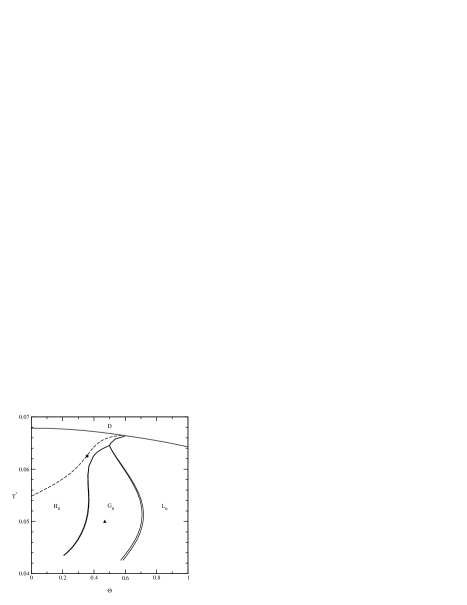
FIG. 1.: X.-j. Li, J. Chem. Phys.

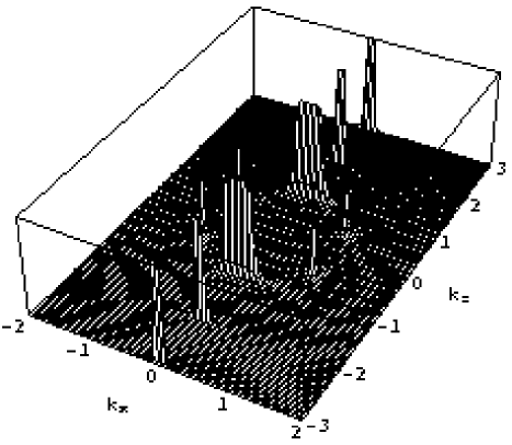
FIG. 2.: X.-j. Li, J. Chem. Phys.

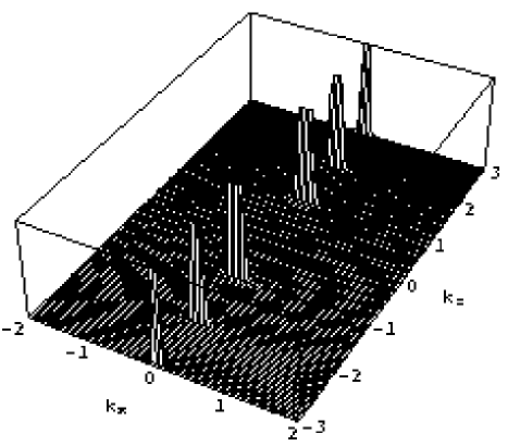
FIG. 3.: X.-j. Li, J. Chem. Phys.

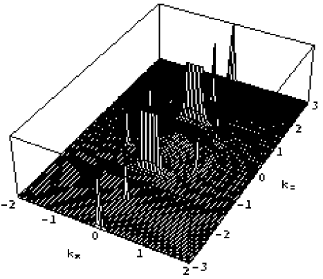
FIG. 4.: X.-j. Li, J. Chem. Phys.

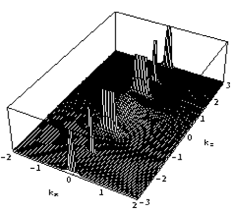
FIG. 5.: X.-j. Li, J. Chem. Phys.

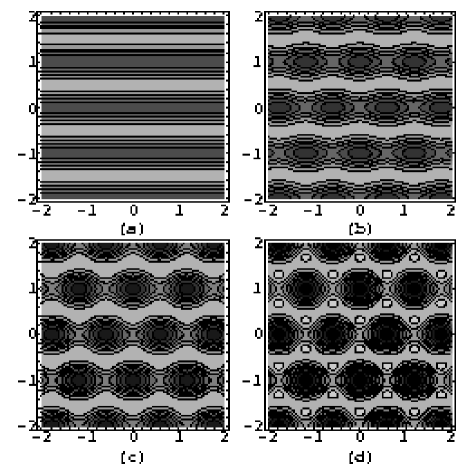
FIG. 6.: X.-j. Li, J. Chem. Phys.

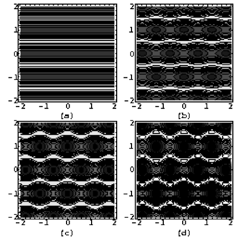
FIG. 7.: X.-j. Li, J. Chem. Phys.

REFERENCES

- [1] P. R. Cullis, M. J. Hope, B. de Kruijff, A. J. Verkleij, and C. P. S. Tilcock, in Phospholipids and Cellular Regulation, edited by J.F. Kuo (CRC Press, Boca Raton 1985), vol. 1, p1.
- [2] B. de Kruijff, Curr. Opin. Chem. Biol. 1, 564 (1997).
- [3] An excellent introduction is provided by Current topics in membranes, vol. 44, edited by R. Epand (Academic, San Diego, 1997).
- [4] S. K. Hui, Chap. 15 in Ref. [3].
- [5] S. L. Keller, S. M. Gruner, and K. Gawrisch, Biochim. Biophys. Acta-Biomembranes 1278, 241 (1996).
- [6] S. M. Bezrukov, R. P. Rand, I. Vodyanoy, and V. A. Parsegian, Faraday Discuss. 111, 173 (1998).
- [7] D. P. Siegel, Biophys. J. 65, 2124 (1993).
- [8] L.V. Chernomordik and J. Zimmerberg, Curr. Opin. in Struct. Biol. 5, 541 (1995).
- [9] M. W. Tate and S. M. Gruner, Biochemistry 26, 231 (1987).
- [10] J. Seddon, Biochim. Biophys. Acta 1031, 1 (1990).
- [11] R. Sundler, N. Düzgünes, and D. Papahadjopoulos, Biochim. Biophys. Acta 649, 751 (1981).
- [12] X.-j. Li and M. Schick, Biophys. J. 78, 34 (2000).
- [13] K. Gawrisch, V. A. Parsegian, D. A. Hadjuk, M. W. Tate, S. M. Gruner, N. L. Fuller, and R. P. Rand, Biochemistry 31, 2856 (1992).
- [14] M. M. Kozlov, S. Leiken, and R. P. Rand, Biophys. J. 67, 1603 (1994).
- [15] X.-j. Li and M. Schick, J. Chem. Phys. (April 1, 2000).
- [16] S. M. Gruner, J. Phys. Chem 93, 7562 (1989).
- [17] S. W. Hui, T. P. Stewart, and L. T. Boni, Chemistry and Physics of Lipids 33, 113 (1983).
- [18] M. Caffrey, Biochemistry 24, 4826 (1985).
- [19] S. M. Gruner, K. J. Rothchild, and W. A. Clark, Biophys. J. 39, 241 (1982).
- [20] A.-C. Shi, J. Noolandi, and R. C. Desai, Macromolecules 29, 6487 (1996).
- [21] M. Laradji, A.-C. Shi, J. Noolandi, and R. C. Desai, Macromolecules 30, 3242 (1997).
- [22] F. Schmid, J. Phys. Cond. Matt. 10, 8105 (1998).
- [23] J. M. Seddon, G. Cevc, and D. Marsh, Biochemistry 22, 1280 (1983).
- [24] M. W. Matsen, Phys. Rev. Lett. 74, 4225 (1995).
- [25] R. P. Rand and N. L. Fuller, Biophys. J. 66, 2127 (1994).
- [26] L. T. Boni and S. W. Hui, Biochim. Biophys. Acta 731, 177 (1983).
- [27] P.-O. Eriksson, L. Rilfors, G. Lindblom, and G. Arvidson, Chemistry and Physics of Lipids 37, 357 (1985).
- [28] D. A. Hajduk, H. Takenouchi, M. A. Hillmyer, F. S. Bates, M. E. Vigild, and K. Almdal, Macromolecules 30, 3788 (1997).
- [29] S. Qi and Z.-G. Wang, Phys. Rev. E 55, 1682 (1997).
- [30] R. R. Netz and M. Schick, Phys. Rev. E 53, 3875 (1996).
- [31] M. Müller and M. Schick, J. Chem. Phys. 105, 8282 (1996).
- [32] V. S. Markin, M. M. Kozlov, V. L. Borovjagin, Gen. Physiol. Biophys. 5, 361 (1984).
- [33] L. Chernomordik, M. M. Kozlov, and J. Zimmerberg, J. Membrane Biol. 146, 1 (1995).
- [34] A. J. Verkleij, C. J. A. Van Echteld, W. J. Gerritsen, P. R. Cullis, and B. de Kruijff, Biochim. Biophys. Acta 600, 620 (1980).
- [35] D. P. Siegel, Biophys. J. 49, 1155 (1986).
- [36] D. P. Siegel and R. M. Epand, Biophys. J. 73, 3089 (1997).