Congested Traffic States in Empirical Observations and Microscopic Simulations

Abstract

We present data from several German freeways showing different kinds of congested traffic forming near road inhomogeneities, specifically lane closings, intersections, or uphill gradients. The states are localized or extended, homogeneous or oscillating. Combined states are observed as well, like the coexistence of moving localized clusters and clusters pinned at road inhomogeneities, or regions of oscillating congested traffic upstream of nearly homogeneous congested traffic. The experimental findings are consistent with a recently proposed theoretical phase diagram for traffic near on-ramps [D. Helbing, A. Hennecke, and M. Treiber, Phys. Rev. Lett. 82, 4360 (1999)]. We simulate these situations with a novel continuous microscopic single-lane model, the “intelligent driver model” (IDM), using the empirical boundary conditions. All observations, including the coexistence of states, are qualitatively reproduced by describing inhomogeneities with local variations of one model parameter. We show that the results of the microscopic model can be understood by formulating the theoretical phase diagram for bottlenecks in a more general way. In particular, a local drop of the road capacity induced by parameter variations has practically the same effect as an on-ramp.

I Introduction

Recently, there is much interest in the dynamics of traffic breakdowns behind bottlenecks [1, 2, 3, 4, 5, 6, 7, 8, 9, 10, 11, 12, 13, 14, 15]. Measurements of traffic breakdowns on various freeways in the USA [13, 1, 2, 6], Germany, [3, 4, 16, 17], Holland [18, 19, 20, 21, 22], and Korea [12] suggest that many dynamic aspects are universal and therefore accessible to a physical description. One common property is the capacity drop (typically of the order of 20%) associated with a breakdown [1, 13, 6], which leads to hysteresis effects and is the basis of applications like dynamic traffic control with the aim of avoiding the breakdown. In the majority of cases, traffic breaks down upstream of a bottleneck and the congestion has a stationary donstream front at the bottleneck. The type of bottleneck, e.g., on-ramps [2, 13, 12, 4], lane closings, or uphill gradients [17], seems not to be of importance. Several types of congested traffic have been found, among them extended states with a relatively high traffic flow. These states, sometimes referred to as “synchronized traffic” [4], can be more or less homogeneously flowing, or show distinct oscillations in the time series of detector data [3]. Very often, the congested traffic flow is, apart from fluctuations, homogeneous near the bottleneck, but oscillations occur further upstream [7]. In other cases, one finds isolated stop-and-go waves that propagate in the upstream direction with a characteristic velocity of about 15 km/h [23, 16]. Finally, there is also an observation of a traffic breakdown to a pinned localized cluster near an on-ramp [12].

There are several possibilities to delineate traffic mathematically, among them macroscopic models describing the dynamics in terms of aggregate quantities like density or flow [24, 25, 26, 27, 10], and microsopic models describing the motion of individual vehicles. The latter include continuous-in-time models (car-following models) [28, 29, 30, 31, 32, 33, 34, 35, 36, 37], and cellular automata [38, 39, 40, 41, 42, 43]. Traffic breakdowns behind bottlenecks have been simulated with the non-local, gaskinetic-based traffic model (GKT model) [27], the Kühne-Kerner-Konhäuser-Lee model (KKKL model) [44, 26, 10], and with a new car-following model, which will be reported below.

For a direct comparison with empirical data, one would prefer car-following models. As the position and velocity of each car is known in such models, one can reconstruct the way how data are obtained by usual induction-loop detectors. To this end, one introduces “virtual” detectors recording passage times and velocities of crossing vehicles and compares this ouput with the empirical data. Because traffic density is not a primary variable, this avoids the problems associated with determining the traffic density by temporal averages [18].

The present study refers to publication [14], where, based on a gas-kinetic-based macroscopic simulation model, it has been concluded that there should be five different congested traffic states on freeways with inhomogeneities like on-ramps. The kind of congested state depends essentially on the inflow into the considered freeway section and on the “bottleneck strength” characterizing the inhomogeneity. This can be summarized by a phase diagram depicting the kind of traffic state as a function of these two parameters. A similar phase diagram has been obtained for the KKKL model [11]. The question is, whether this finding is true for some macroscopic models only, or universal for a larger class of traffic models and confirmed by empirical data.

The relative positions of some of the traffic states in this phase space has been qualitatively confirmed for a Korean freeway [12], but only one type of extended state has been measured there. Furthermore, this state did not have the characteristic properties of extended congested traffic on most other freeways, cf. e.g., [4]. It is an open question to confirm the relative position of the other states. Moreover, to our knowledge, there are no direct simulations of the different breakdowns using empirical data as boundary conditions, neither with microscopic nor with macroscopic models.

Careful investigations with a new follow-the-leader model (the IDM model) [36, 37] show that (i) the conclusions of Ref [14] are also valid for certain microscopic traffic models (at least deterministic models with a metastable density range), (ii) the results can be systematically transferred to more general (in particular flow-conserving) kinds of bottlenecks, and a formula allowing to quantify the bottleneck strength is given [see Eq. (15)], (iii) the existence of all predicted traffic states is empirically supported, and finally, (iv) all different kinds of breakdowns can be simulated with the IDM model with empirically measured boundary conditions, varying only one parameter (the average time headway T), which is used to specify the capacity of the stretch.

The applied IDM model belongs to the class of deterministic follow-the-leader models like the optimal velocity model by Bando et al. [31], but it has the following advantages: (i) it behaves accident-free because of the dependence on the relative velocity, (ii) for similar reasons and because of metastability, it shows the self-organized characteristic traffic constants demanded by Kerner et al. [26] (see Fig. 4), hysteresis effects [45, 13], and complex states [3, 7], (iii) all model parameters have a reasonable interpretation, are known to be relevant, are empirically measurable, and have the expected order of magnitude [37], (iv) the fundamental diagram and the stability properties of the model can be easily (and separately) calibrated to empirical data, (v) it allows for a fast numerical simulation, and (vi) an equivalent macroscopic version of the model is known [46], which is not the case for most other microscopic traffic models.

These aspects are discussed in Sec. II, while Sec. III is not model-specific at all. Section III presents ways to specify and quantify bottlenecks, as well as the traffic states resulting for different traffic volumes and bottleneck strengths. The analytical expressions for the phase boundaries of the related phase diagram allow to conclude that similar results will be found for any other traffic model with a stable, metastable, and unstable density range. Even such subtle features like tristability first found in macroscopic models [11, 37] are observed. It would be certainly interesting to investigate in the future, whether the same phenomena are also found for CA models or stochastic traffic models like the one by Krauss [32].

Section IV discusses empirical data using representative examples out of a sample of about 100 investigated breakdowns. Thanks to a new method for presenting the cross section data (based on a smoothing and interpolation procedure), it is possible to present 3d plots of the empirical density or average velocity as a function of time and space. This allows a good imagination of the traffic patterns and a direct visual comparison with simulation results. In the IDM microsimulations, we used a very restricted data set, namely only the measured flows and velocities at the upstream and downstream boundaries omitting the data of the up to eight detectors in between. Although the simulated sections were up to 13 km long and the boundaries were typically outside of congestions, the simulations reproduced qualitatively the sometimes very complex observed collective dynamics.

All in all the study supports the idea of the suggested phase diagram of congested traffic states quite well and suggests ways to simulate real traffic breakdowns at bottlenecks with empirical boundary conditions.

II The Microscopic “Intelligent Driver Model” (IDM)

For about fifty years now, researchers model freeway traffic by means of continuous-in-time microscopic models (car-following models) [47]. Since then, a multitude of car-following models have been proposed, both for single-lane and multi-lane traffic including lane changes. We will restrict, here, to phenomena for which lane changes are not important and only consider single-lane models. To motivate our traffic model we first give an overview of the dynamical properties of some popular microscopic models.

A Dynamic Properties of Some Car-Following Models

Continuous-time single-lane car-following models are defined essentially by their acceleration function. In many of the earlier models [48, 49, 50, 51], the acceleration $\dot{v}_{\alpha}(t+T_{r})$ of vehicle $\alpha$, delayed by a reaction time $T_{r}$, can be written as

$$\dot{v}_{\alpha}(t+T_{r})=\frac{-\lambda v_{\alpha}^{m}\Delta v_{\alpha}}{s_{\alpha}^{l}}.$$ (1)

The deceleration $-\dot{v}_{\alpha}(t+T_{r})$ is asumed to be proportional to the approaching rate

$$\Delta v_{\alpha}(t):=v_{\alpha}(t)-v_{\alpha-1}(t)$$ (2)

of vehicle $\alpha$ with respect to the leading vehicle $(\alpha-1)$. In addition, the acceleration may depend on the own velocity $v_{\alpha}$ [50] and decrease with some power of the net (bumper-to-bumper) distance

$$s_{\alpha}=x_{\alpha-1}-x_{\alpha}-l_{\alpha}$$ (3)

to the leading vehicle (where $l_{\alpha}$ is the vehicle length) [50, 51]. Since, according to Eq. (1), the acceleration depends on a leading vehicle, these models are not applicable for very low traffic densities. If no leading vehicle is present (corresponding to $s_{\alpha}\to\infty$), the acceleration is either not determined $(l=0)$ or zero $(l>0)$, regardless of the own velocity. However, one would expect in this case that drivers accelerate to an individual desired velocity. The car-following behavior in dense traffic is also somewhat unrealistic. In particular, the gap $s_{\alpha}$ to the respective front vehicle does not necessarily relax to an equilibrium value. Even small gaps will not induce braking reactions if the velocity difference $\Delta v_{\alpha}$ is zero.

These problems are solved by the car-following model of Newell [28]. In this model, the velocity at time $(t+T_{r})$ depends adiabatically on the gap, i.e., the vehicle adapts exactly to a distance-dependent function $V$ within the reaction time $T_{r}$,

$$v_{\alpha}(t+T_{r})=V\Big{(}s_{\alpha}(t)\Big{)}.$$ (4)

The “optimal velocity function” $V(s)=v_{0}\{1-\exp[-(s-s_{0})/(v_{0}T)]\}$ includes both, a desired velocity $v_{0}$ for vanishing interactions ($s\to\infty$) and a safe time headway $T$ characterizing the car-following behavior in dense (equilibrium) traffic. The Newell model is collision-free, but the immediate dependence of the velocity on the density leads to very high accelerations of the order of $v_{0}/T_{r}$. Assuming a typical desired velocity of 30 m/s and $T_{r}=1$ s, this would correspond to 30 m/s², which is clearly unrealistic [33, 52].

More than 30 years later, Bando et al. suggested a similar model,

$$\dot{v}_{\alpha}=\frac{V(s_{\alpha})-v_{\alpha}}{\tau}$$ (5)

with a somewhat different optimal velocity function. This “optimal-velocity mdoel” has been widely used by physicists because of its simplicity, and because some results could be derived analytically. The dynamical behavior does not greatly differ from the Newell model, since the reaction time delay $T_{r}$ of the Newell model can be compared with the velocity relaxation time $\tau$ of the optimal-velocity model. However, realistic velocity relaxation times are of the order of 10 s (city traffic) to 40 s (freeway traffic) and therefore much larger than reaction delay times (of the order of 1 s). For typical values of the other parameters of the optimal-velocity model [31], crashes are only avoided if $\tau<0.9$ s, i.e., the velocity relaxation time is of the order of the reaction time, leading again to unrealistically high values $v_{0}/\tau$ of the maximum acceleration. The reason of this unstable behavior is that effects of velocity differences are neglected. However, they play an essential stabilizing role in real traffic, especially when approaching traffic jams. Moreover, in models (4) and (5), accelerations and decelerations are symmetric with respect to the deviation of the actual velocity from the equilibrium velocity, which is unrealistic. The absolute value of braking decelerations is usually stronger than that of accelerations.

A relatively simple model with a generalized optimal velocity function incorporating both, reactions to velocity differences and different rules for acceleration and braking has been proposed rather recently [33]. This “generalized-force model” could successfully reproduce the time-dependent gaps and velocities measured by a sensor-equipped car in congested city traffic. However, the acceleration and deceleration times in this model are still unrealistically small which requires inefficiently small time steps for the numerical simulation.

Besides these simple models intended for basic investigations, there are also highly complex “high-fidelity models” like the Wiedemann model [30] or MITSIM [34], which try to reproduce traffic as realistically as possible, but at the cost of a large number of parameters.

Other approaches that incorporate “intelligent” and realistic braking reactions are the simple and fast stochastic models proposed by Gipps [29, 53] and Krauss [32]. Despite their simplicity, these models show a realistic driver behavior, have asymmetric accelerations and decelerations, and produce no accidents. Unfortunately, they lose their realistic properties in the deterministic limit. In particular, they show no traffic instabilities or hysteresis effects for vanishing fluctuations.

B Model Equations

The acceleration assumed in the IDM is a continuous function of the velocity $v_{\alpha}$, the gap $s_{\alpha}$, and the velocity difference (approaching rate) $\Delta v_{\alpha}$ to the leading vehicle:

$$\dot{v}_{\alpha}=a^{(\alpha)}\left[1-\left(\frac{v_{\alpha}}{v_{0}^{(\alpha)}}\right)^{\delta}-\left(\frac{s^{*}(v_{\alpha},\Delta v_{\alpha})}{s_{\alpha}}\right)^{2}\right].$$ (6)

This expression is an interpolation of the tendency to accelerate with $a_{f}(v_{\alpha}):=a^{(\alpha)}[1-(v_{\alpha}/v_{0}^{(\alpha)})^{\delta}]$ on a free road and the tendency to brake with deceleration $-b_{\rm int}(s_{\alpha},v_{\alpha},\Delta v_{\alpha}):=-a^{(\alpha)}(s^{*}/s_{\alpha})^{2}$ when vehicle $\alpha$ comes too close to the vehicle in front. The deceleration term depends on the ratio between the “desired minimum gap” $s^{*}$ and the actual gap $s_{\alpha}$, where the desired gap

$$s^{*}(v,\Delta v)=s_{0}^{(\alpha)}+s_{1}^{(\alpha)}\sqrt{\frac{v}{v_{0}^{(\alpha)}}}+T^{\alpha}v+\frac{v\Delta v}{2\sqrt{a^{(\alpha)}b^{(\alpha)}}}$$ (7)

is dynamically varying with the velocity and the approaching rate.

In the rest of this paper, we will study the case of identical vehicles whose model parameters $v_{0}^{(\alpha)}=v_{0}$, $s_{0}^{(\alpha)}=s_{0}$, $T^{(\alpha)}=T$, $a^{(\alpha)}=a$, $b^{(\alpha)}=b$, and $\delta$ are given in Table I. Here, our emphasis is on basic investigations with models as simple as possible, and therefore we will set $s_{1}^{\alpha}=0$ resulting in a model where all parameters have an intuitive meaning with plausible and often easily measurable values. While the empirical data presented in this paper can be nevertheless reproduced, a distinction of different driver-vehicle types and/or a nonzero $s_{1}$ [37] is necessary for a more quantitative agreement. A nonzero $s_{1}$ would also be necessary for features requiring an inflection point in the equilibrium flow-density relation, e.g., for certain types of multi-scale expansions [54].

C Dynamic Single-Vehicle Properties

Special cases of the IDM acceleration (6) with $s_{1}=0$ include the following driving modes:

a Equilibrium traffic:

In equilibrium traffic of arbitrary density ($\dot{v}_{\alpha}=0$, $\Delta v_{\alpha}=0$), drivers tend to keep a velocity-dependent equilibrium gap $s_{e}(v_{\alpha})$ to the front vehicle given by

$$s_{e}(v)=s^{*}(v,0)\left[1-\left(\frac{v}{v_{0}}\right)^{\delta}\right]^{-\frac{1}{2}}=(s_{0}+vT)\left[1-\left(\frac{v}{v_{0}}\right)^{\delta}\right]^{-\frac{1}{2}}.$$ (8)

In particular, the equilibrium gap of homogeneous congested traffic (with $v_{\alpha}\ll v_{0}$) is essentially equal to the desired gap, $s_{e}(v)\approx s_{0}+vT$, i.e., it is composed of a bumper-to-bumper space $s_{0}$ kept in standing traffic and an additional velocity-dependent contribution $vT$ corresponding to a constant safe time headway $T$. This high-density limit is of the same functional form as that of the Newell model, Eq. (4). Solving Eq. (8) for $v:=V_{e}(s)$ leads to simple expressions only for $\delta=1$, $\delta=2$, or $\delta\to\infty$. In particular, the equilibium velocity for $\delta=1$ and $s_{0}=0$ is

$$V_{e}(s)|_{\delta=1,s_{0}=0}=\frac{s^{2}}{2v_{0}T^{2}}\left(-1+\sqrt{1+\frac{4T^{2}v_{0}^{2}}{s^{2}}}\right).$$ (9)

Further interesting cases are

$$V_{e}(s)|_{\delta=2,s_{0}=0}=\frac{v_{0}}{\sqrt{1+\frac{v_{0}^{2}T^{2}}{s^{2}}}},$$ (10)

and

$$V_{e}(s)|_{\delta\to\infty}=\mbox{min}\{v_{0},(s-s_{0})/T\}.$$ (11)

From a macroscopic point of view, equilibrium traffic consisting of identical vehicles can be characterized by the equilibrium traffic flow $Q_{e}(\rho)=\rho V_{e}(\rho)$ (vehicles per hour and per lane) as a function of the traffic density $\rho$ (vehicles per km and per lane). For the IDM model, this “fundamental diagram” follows from one of the equilibrium relations (8) to (11), together with the micro-macro relation between gap and density:

$$s=1/\rho-l=1/\rho-1/\rho_{\rm max}.$$ (12)

Herein, the maximum density $\rho_{\rm max}$ is related to the vehicle length $l$ by $\rho_{\rm max}l=1$. Figure 1 shows the fundamental diagram and its dependence on the parameters $\delta$, $v_{0}$, and $T$. In particular, the fundamental diagram for $s_{0}=0$ and $\delta=1$ is identical to the equilibrium relation of the macroscopic GKT model, if the GKT parameter $\Delta A$ is set to zero (cf. Eq. (23) in Ref. [27]), which is a necessary condition for a micro-macro correspondence [46].

b Acceleration to the desired velocity:

If the traffic density is very low ($s$ is large), the interaction term is negligible and the IDM acceleration reduces to the free-road acceleration $a_{f}(v)=a(1-v/v_{0})^{\delta}$, which is a decreasing function of the velocity with a maximum value $a_{f}(0)=a$ and $a_{f}(v_{0})=0$. In Fig. 2, this regime applies for times $t\leq 60$ s. The acceleration exponent $\delta$ specifies how the acceleration decreases when approaching the desired velocity. The limiting case $\delta\to\infty$ corresponds to approaching $v_{0}$ with a constant acceleration $a$, while $\delta=1$ corresponds to an exponential relaxation to the desired velocity with the relaxation time $\tau=v_{0}/a$. In the latter case, the free-traffic acceleration is equivalent to that of the optimal-velocity model (5) and also to acceleration functions of many macroscopic models like the KKKL model [26], or the GKT model [27]. However, the most realistic behavior is expected in between the two limiting cases of exponential acceleration (for $\delta=1$) and constant acceleration (for $\delta\rightarrow\infty$), which is confirmed by our simulations with the IDM. Throughout this paper we will use $\delta=4$.

c Braking as reaction to high approaching rates:

When approaching slower or standing vehicles with sufficiently high approaching rates $\Delta v>0$, the equilibrium part $s_{0}+vT$ of the dynamical desired distance $s^{*}$, Eq. (7), can be neglected with respect to the nonequilibrium part, which is proportional to $v\Delta v$. Then, the interaction part $-a(s^{*}/s)^{2}$ of the acceleration equation (6) is given by

$$b_{\rm int}(s,v,\Delta v)\approx\frac{(v\Delta v)^{2}}{4bs^{2}}.$$ (13)

This expression implements anticipative “intelligent” braking behavior, which we disuss now for the spacial case of approaching a standing obstacle ($\Delta v=v$). Anticipating a constant deceleration during the whole approaching process, a minimum kinematic deceleration $b_{k}:=v^{2}/(2s)$ is necessary to avoid a collision. The situation is assumed to be “under control”, if $b_{k}$ is smaller than the “comfortable” deceleration given by the model parameter $b$, i.e., $\beta:=b_{k}/b\leq 1$. In contrast, an emergency situation is characterized by $\beta>1$. With these definitions, Eq. (13) becomes

$$b_{\rm int}(s,v,v)=\frac{b_{k}^{2}}{b}=\beta b_{k}.$$ (14)

While in safe situations the IDM deceleration is less than the kinematic collision-free deceleration, drivers overreact in emergency situations to get the situation again under control. It is easy to show that in both cases the acceleration approaches $\dot{v}=-b$ under the deceleration law (14). Notice that this stabilizing behavior is lost if one replaces in Eq. (6) the braking term $-a(s^{*}/s)^{2}$ by $-a^{\prime}(s^{*}/s)^{\delta^{\prime}}$ with $\delta^{\prime}\leq 1$ corresponding to $b_{\rm int}(s,v,v)=\beta^{\delta^{\prime}-1}b_{k}$. The “intelligent” braking behavior of drivers in this regime makes the model collision-free. The right parts of the plots of Fig. 2 ($t>70$ s) show the simulated approach of an IDM vehicle to a standing obstacle. As expected, the maximum deceleration is of the order of $b$. For low velocities, however, the equilibrium term $s_{0}+vT$ of $s^{*}$ cannot be neglected as assumed when deriving Eq. (14). Therefore, the maximum deceleration is somewhat lower than $b$ and the deceleration decreases immediately before the stop while, under the dynamics (14), one would have $\dot{v}=-b$.

Similar braking rules have been implemented in the model of Krauss [32], where the model is formulated in terms of a time-discretizised update scheme (iterated map), where the velocity at timestep $(t+1)$ is limited to a “safe velocity” which is calculated on the basis of the kinematic braking distance at a given “comfortable” deceleration.

d Braking in response to small gaps:

The forth driving mode is active when the gap is much smaller than $s^{*}$ but there are no large velocity differences. Then, the equilibrium part $s_{0}+vT$ of $s^{*}$ dominates over the dynamic contribution proportional to $\Delta v$. Neglecting the free-road acceleration, Eq. (6) reduces to $\dot{v}\approx-(s_{0}+vT)^{2}/s^{2}$, corresponding to a Coulomb-like repulsion. Such braking interactions are also implemented in other models, e.g., in the model of Edie [51], the GKT model [27], or in certain regimes of the Wiedemann model [30]. The dynamics in this driving regime is not qualitatively different, if one replaces $-a(s^{*}/s)^{2}$ by $-a(s^{*}/s)^{\delta^{\prime}}$ with $\delta^{\prime}>0$. This is in contrast to the approaching regime, where collisions would be provoked for $\delta^{\prime}\leq 1$. Figure 3 shows the car-following dynamics in this regime. For the standard parameters, one clearly sees an non-oscillatory relaxation to the equilibrium distance (solid curve), while for very high values of $b$, the approach to the equilibrium distance would occur with damped oscillations (dashed curve). Notice that, for the latter parameter set, the collective traffic dynamics would already be extremely unstable.

D Collective Behavior and Stability Diagram

Although we are interested in realistic open traffic systems, it turned out that many features can be explained in terms of the stability behavior in a closed system. Figure 4(a) shows the stability diagram of homogeneous traffic on a circular road. The control parameter is the homogeneous density $\rho_{\rm h}$. We applied both a very small and a large localized perturbation to check for linear and nonlinear stability, and plotted the resulting minimum ($\rho_{\rm out}$) and maximum ($\rho_{\rm jam}$) densities after a stationary situation was reached. The resulting diagram is very similar to that of the macroscopic KKKL and GKT models [26, 27]. In particular, it displays the following realistic features: (i) Traffic is stable for very low and high densities, but unstable for intermediate densities. (ii) There is a density range $\rho_{\rm c1}\leq\rho_{\rm h}\leq\rho_{\rm c2}$ of metastability, i.e., only perturbations of sufficiently large amplitudes grow, while smaller perturbations disappear. Note that, for most IDM parameter sets, there is no second metastable range at higher densities, in contrast to the GKT and KKKL models. Rather, traffic flow becomes stable again for densities exceeding the critical density $\rho_{\rm c3}$, or congested flows below $Q_{\rm c3}=Q_{\rm e}(\rho_{\rm c3})$. (iii) The density $\rho_{\rm jam}$ inside of traffic jams and the associated flow $Q_{\rm jam}=Q_{\rm e}(\rho_{\rm jam})$, cf. Fig. 4(b), do not depend on $\rho_{\rm h}$. For the parameter set chosen here, we have $\rho_{\rm jam}=\rho_{\rm c3}=140$ vehicles/km, and $Q_{\rm jam}=0$, i.e., there is no linearly stable congested traffic with a finite flow and velocity. For other parameters, especially for a nonzero IDM parameter $s_{1}$, both $Q_{\rm jam}$ and $Q_{\rm c3}$ can be nonzero and different from each other [37].

As further “traffic constants”, at least in the density range 20 veh./km $\leq\rho_{\rm h}\leq$ 50 veh./km, we observe a constant outflow $Q_{\rm out}=Q_{\rm e}(\rho_{\rm out})$ and propagation velocity $v_{\rm g}=(Q_{\rm out}-Q_{\rm jam})/(\rho_{\rm out}-\rho_{\rm jam})\approx-15$ km/h of traffic jams. Figure 4(b) shows the stability diagram for the flows. In particular, we have $Q_{\rm c1}<Q_{\rm out}\approx Q_{\rm c2}$, where $Q_{{\rm c}i}=Q_{\rm e}(\rho_{{\rm c}i})$, i.e., the outflow from congested traffic is at the margin of linear stability, which is also the case in the GKT for most parameter sets [27, 14]. For other IDM parameters, the outflow $Q_{\rm out}\in[Q_{\rm c1},Q_{\rm c2}]$ is metastable [37], or even at the margin of nonlinear stability [36].

In open systems, a third type of stability becomes relevant. Traffic is convectively stable, if, after a sufficiently long time, all perturbations are convected out of the system. Both, in the macroscopic models and in the IDM, there is a considerable density region $\rho_{\rm cv}\leq\rho_{\rm h}\leq\rho_{\rm c3}$, where traffic is linearly unstable but convectively stable. For the parameters chosen in this paper, congested traffic is always linearly unstable, but convectively stable for flows below $Q_{\rm cv}=Q_{\rm e}(\rho_{\rm cv})=1050$ vehicles/h. A nonzero jam distance $s_{1}$ is required for linearly stable congested traffic with nonzero flows [37], at least, if the model should simultaneously show traffic instabilities.

E Calibration

Besides the vehicle length $l$, the IDM has seven parameters, cf. Table I. The fundamental relations of homogeneous traffic are calibrated with the desired velocity $v_{0}$ (low density), safe time headway $T$ (high density), and the jam distances $s_{0}$ and $s_{1}$ (jammed traffic). In the low-density limit $\rho\ll(v_{0}T)^{-1}$, the equilibrium flow can be approximated by $Q_{e}\approx V_{0}\rho$. In the high density regime and for $s_{1}=0$, one has a linear decrease of the flow $Q_{e}\approx[1-\rho(l+s_{0})]/T$ which can be used to determine $(l+s_{0})$ and $T$. Only for nonzero $s_{1}$, one obtains an inflection point in the equilibrium flow-density relation $Q_{e}(\rho)$. The acceleration coefficient $\delta$ influences the transition region between the free and congested regimes. For $\delta\to\infty$ and $s_{1}=0$, the fundamental diagram (equilibrium flow-density relation) becomes triangular-shaped: $Q_{e}(\rho)=\mbox{min}(v_{0}\rho,[1-\rho(l+s_{0})]/T)$. For decreasing $\delta$, it becomes smoother and smoother, cf. Fig. 1(a).

The stability behavior of traffic in the IDM model is determined mainly by the maximum acceleration $a$, desired deceleration $b$, and by $T$. Since the accelerations $a$ and $b$ do not influence the fundamental diagram, the model can be calibrated essentially independently with respect to traffic flows and stability. As in the GKT model, traffic becomes more unstable for decreasing $a$ (which corresponds to an increased acceleration time $\tau=v_{0}/a$), and with decreasing $T$ (corresponding to reduced safe time headways). Furthermore, the instability increases with increasing $b$. This is also plausible, because an increased desired deceleration $b$ corresponds to a less anticipative or less defensive braking behavior. The density and flow in jammed traffic and the outflow from traffic jams is also influenced by $s_{0}$ and $s_{1}$. In particular, for $s_{1}=0$, the traffic flow $Q_{\rm jam}$ inside of traffic jams is typically zero after a sufficiently long time [Fig. 4(b)], but nonzero otherwise. The stability of the self-organized outflow $Q_{\rm out}$ depends strongly on the minimum jam distance $s_{0}$. It can be unstable (small $s_{0}$), metastable, or stable (large $s_{0}$). In the latter case, traffic instabilities can only lead to single localized clusters, not to stop-and go traffic.

III Microscopic Simulation of Open Systems with an Inhomogeneity

We simulated identical vehicles of length $l=5$ m with the typical IDM model parameters listed in Table I. Moreover, although the various congested states discussed in the following were observed on different freeways, all of them were qualitatively reproduced with very restrictive variations of one single parameter (the safe time headway $T$), while we always used the same values for the other parameters (see Table I). This indicates that the model is quite realistic and robust. Notice that all parameters have plausible values. The value $T=1.6$ s for the safe time headway is slightly lower than suggested by German authorities (1.8 s). The acceleration parameter $a=0.73$ m/s² corresponds to a free-road acceleration from $v=0$ to $v=100$ km/h within 45 s, cf. Fig. 2(b). This value is obtained by integrating the IDM acceleration $\dot{v}=a[1-(v/v_{0})^{\delta}]$ with $v_{0}=120$ km/h, $\delta=4$, and the initial value $v(0)=0$. While this is considerably above minimum acceleration times (10 s - 20 s for average-powered cars), it should be characteristic for everyday accelerations. The comfortable deceleration $b=1.67$ m/s² is also consistent with empirical investigations [52, 33], and with parameters used in more complex models [34].

With efficient numerical integration schemes, we obtained a numerical performance of about $10^{5}$ vehicles in realtime on a usual workstation [55].

A Modelling of Inhomogeneities

Road inhomogeneities can be classified into flow-conserving local defects like narrow road sections or gradients, and those that do not conserve the average flow per lane, like on-ramps, off-ramps, or lane closings.

Non-conserving inhomogeneities can be incorporated into macroscopic models in a natural way by adding a source term to the continuity equation for the vehicle density [56, 8, 10]. An explicit microscopic modelling of on-ramps or lane closings, however, would require a multi-lane model with an explicit simulation of lane changes. Another possibility opened by the recently formulated micro-macro link [46] is to simulate the ramp section macroscopically with a source term in the continuity equation [8], and to simulate the remaining stretch microscopically.

In contrast, flow conserving inhomogeneities can be implemented easily in both microscopic and macroscopic single-lane models by locally changing the values of one or more model parameters or by imposing external decelerations [5]. Suitable parameters for the IDM and the GKT model are the desired velocity $v_{0}$, or the safe time headway $T$. Regions with locally decreased desired velocity can be interpreted either as sections with speed limits, or as sections with uphill gradients (limiting the maximum velocity of some vehicles) [57]. Increased safe time headways can be attributed to more careful driving behavior along curves, on narrow, dangerous road sections, or a reduced range of visibility.

Local parameter variations act as a bottleneck, if the outflow $Q^{\prime}_{\rm out}$ from congested traffic (dynamic capacity) in the downstream section is reduced with respect to the outflow $Q_{\rm out}$ in the upstream section. This outflow can be determined from fully developed stop-and go waves in a closed system, whose outflow is constant in a rather large range of average densities $\rho_{\rm h}\in$ [20 veh./km, 60 veh./km], cf. Fig. 4(b). It will turn out that the outflow $Q^{\prime}_{\rm out}$ is the relevant capacity for understanding congested traffic, and not the maximum flow $Q_{\rm max}$ (static capacity), which can be reached in (spatially homogeneous) equilibrium traffic only. The capacities are decreased, e.g., for a reduced desired velocity $v^{\prime}_{0}<v_{0}$ or an increased safe time headway $T^{\prime}>T$, or both. Figure 5 shows $Q_{\rm out}$ and $Q_{\rm max}$ as a function of $T$. For $T^{\prime}>4$ s, traffic flow is always stable, and the outflow from jams is equal to the static capacity.

For extended congested states, all types of flow-conserving bottlenecks result in a similar traffic dynamics, if $\delta Q=(Q_{\rm out}-Q^{\prime}_{\rm out})$ is identical, where $Q^{\prime}_{\rm out}$ is the outflow for the changed model parameters $v_{0}^{\prime}$, $T^{\prime}$, etc. Qualitatively the same dynamics is also observed in macroscopic models including on-ramps, if the ramp flow satisfies $Q_{\rm rmp}\approx\delta Q$ [37]. This suggests to introduce the following general definition of the “bottleneck strength” $\delta Q$:

$$\delta Q:=Q_{\rm rmp}+Q_{\rm out}-Q^{\prime}_{\rm out},$$ (15)

In particular, we have $\delta Q=Q_{\rm rmp}$ for on-ramp bottlenecks, and $\delta Q=(Q_{\rm out}-Q^{\prime}_{\rm out})$ for flow-conserving bottlenecks, but formula (15) is also applicable for a combination of both.

B Phase Diagram of Traffic States in Open Systems

In contrast to closed systems, in which the long-term behavior and stability is essentially determined by the average traffic density $\rho_{h}$, the dynamics of open systems is controlled by the inflow $Q_{\rm in}$ to the main road (i.e., the flow at the upstream boundary). Furthermore, traffic congestions depend on road inhomogeneities and, because of hysteresis effects, on the history of previous perturbations.

In this paper, we will implement flow-conserving inhomogeneities by a variable safe time headway $T(x)$. We chose $T$ as variable model parameter because it influences the flows more effectively than $v_{0}$, which has been varied in Ref. [37]. Specifically, we increase the local safe time headway according to

$$T(x)=\left\{\begin{array}[]{ll}T&\ \ x\leq-L/2\\ T^{\prime}&\ \ x\geq L/2\\ T+(T^{\prime}-T)\left(\frac{x}{L}+\frac{1}{2}\right)&\ \ |x|<L/2,\end{array}\right.$$ (16)

where the transition region of length $L=600$ is analogous to the ramp length for inhomogeneities that do not conserve the flow. The bottleneck strength $\delta Q(T^{\prime})=[Q_{\rm out}(T)-Q_{\rm out}(T^{\prime})]$ is an increasing function of $T^{\prime}$, cf. Fig. 5(a). We investigated the traffic dynamics for various points $(Q_{\rm in},\delta Q)$ or, alternatively, $(Q_{\rm in},T^{\prime}-T)$ in the control-parameter space.

Due to hysteresis effects and multistability, the phase diagram, i.e., the asymptotic traffic state as a function of the control parameters $Q_{\rm in}$ and $\Delta T$, depends also on the history, i.e., on initial conditions and on past boundary conditions and perturbations. Since we cannot explore the whole functional space of initial conditions, boundary conditions, and past perturbations, we used the following three representative “standard” histories.

• Assuming very low values for the initial density and flow, we slowly increased the inflow to the prescribed value $Q_{\rm in}$.

• We started the simulation with a stable pinned localized cluster (PLC) state and a consistent value for the inflow $Q_{\rm in}$. Then, we adiabatically changed the inflow to the values prescribed by the point in the phase diagram.

• After running history A, we applied a large perturbation at the downstream boundary. If traffic at the given phase point is metastable, this initiates an upstream propagating localized cluster which finally crosses the inhomogeneity, see Fig. 7(a)-(c). If traffic is unstable, the breakdown already occurs during time period A, and the additional perturbation has no dynamic influence.

For a given history, the resulting phase diagram is unique. The solid lines of Fig. 6 show the IDM phase diagram for History C. Spatio-temporal density plots of the congested traffic states themselfes are displayed in Fig. 7. To obtain the spatiotemporal density $\rho(x,t)$ from the microscopic quantities, we generalize the micro-macro relation (12) to define the density at discrete positions $x_{\alpha}+\frac{l+s_{\alpha}}{2}$ centered between vehicle $\alpha$ and its predecessor,

$$\rho(x_{\alpha}+\frac{l+s_{\alpha}}{2})=\frac{1}{l+s_{\alpha}},$$ (17)

and interpolate linearly between these positions. Depending on $Q_{\rm in}$ and $\delta T:=(T^{\prime}-T)$, the downstream perturbation (i) dissipates, resulting in free traffic (FT), (ii) travels through the inhomogeneity as a moving localized cluster (MLC) and neither dissipates nor triggers new breakdowns, (iii) triggers a traffic breakdown to a pinned localized cluster (PLC), which remains localized near the inhomogeneity for all times and either is stationary (SPLC), cf. Fig. 8(a) for $t<0.2$ h, or oscillatory (OPLC). (iv) Finally, the initial perturbation can induce extended congested traffic (CT), whose downstream boundaries are fixed at the inhomogeneity, while the upstream front propagates further upstream in the course of time. Extended congested traffic can be homogeneous (HCT), oscillatory (OCT), or consist of triggered stop-and-go waves (TSG). We also include in the HCT region a complex state (HCT/OCT) where traffic is homogeneous only near the bottleneck, but growing oscillations develop further upstream. In contrast to OCT, where there is permanently congested traffic at the inhomogeneity (“pinch region” [7, 36]), the TSG state is characterized by a series of isolated density clusters, each of which triggers a new cluster as it passes the inhomogeneity. The maximum perturbation of History C, used also in Ref. [14], seems to select always the stable extended congested phase. We also scanned the control-parameter space $(Q_{\rm in},\delta Q)$ with Histories A and B exploring the maximum phase space of the (meta)stable FT and PLC states, respectively, cf. Fig. 6. In multistable regions of the control-parameter space, the three histories can be used to select the different traffic states, see below.

C Multistability

In general, the phase transitions between free traffic, pinned localized states, and extended congested states are hysteretic. In particular, in all four examples of Fig. 7, free traffic is possible as a second, metastable state. In the regions between the two dotted lines of the phase diagram Fig. 6, both, free and congested traffic is possible, depending on the previous history. In particular, for all five indicated phase points, free traffic would persist without the downstream perturbation. In contrast, the transitions PLC-OPLC, and HCT-OCT-TSG seem to be non-hysteretic, i.e., the type of pinned localized cluster or of extended congested traffic, is uniquely determined by $Q_{\rm in}$ and $\delta Q$.

In a small subset of the metastable region, labelled “TRI” in Fig. 6, we even found tristability with the possible states FT, PLC, and OCT. Figure 8(a) shows that a single moving localized cluster passing the inhomogeneity triggers a transition from PLC to OCT. Starting with free traffic, the same perturbation would trigger OCT as well [Fig. 8(b)], while we never found reverse transitions OCT $\to$ PLC or OCT $\to$ FT (without a reduction of the inflow). That is, FT and PLC are metastable in the tristable region, while OCT is stable. We obtained qualitatively the same also for the macroscopic GKT model with an on-ramp as inhomogeneity [Fig. 8(c)]. Furthermore, tristability between FT, OPLC, and OCT has been found for the IDM model with variable $v_{0}$ [37], and for the KKKL model [11].

Such a tristability can only exist if the (self-organized) outflow $Q_{\rm out}^{\rm OCT}=\tilde{Q}_{\rm out}$ from the OCT state is lower than the maximum outflow $Q_{\rm out}^{\rm PLC}$ from the PLC state. A phenomenological explanation of this condition can be inferred from the positions of the downstream fronts of the OCT and PLC states shown in Fig. 8(a). The downstream front of the OCT state ($t>1$ h) is at $x\approx 300$ m, i.e., at the downstream boundary of the $L=600$ m wide transition region, in which the safe time headway Eq. (16) increases from $T$ to $T^{\prime}>T$. Therefore, the local safe time headway at the downstream front of OCT is $T^{\prime}$, or $Q_{\rm out}^{\rm OCT}\approx Q^{\prime}_{\rm out}$, which was also used to derive Eq. (18). In contrast, the PLC state is centered at about $x=0$, so that an estimate for the upper boundary $Q_{\rm out}^{\rm PLC}$ of the outflow is given by the self-organized outflow $Q_{\rm out}$ corresponding to the local value $T(x)=(T+T^{\prime})/2$ of the safe time headway at $x=0$. Since $(T+T^{\prime})/2<T^{\prime}$ this outflow is higher than $Q_{\rm out}^{\rm OCT}$ (cf. Fig. 5). It is an open question, however, why the downstream front of the OCT state is further downstream compared to the PLC state. Possibly, it can be explained by the close relationship of OCT with the TSG state, for which the newly triggered density clusters even enter the region downstream of the bottleneck [cf. Fig. 7(c)]. In accordance with its relative location in the phase diagram, it is plausible that the OCT state has a “penetration depth” into the downstream area that is in between the one of the PLC and the TSG states.

D Boundaries between and Coexistence of Traffic States

Simulations show that the outflow $\tilde{Q}_{\rm out}$ from the nearly stationary downstream fronts of OCT and HCT satisfies $\tilde{Q}_{\rm out}\leq Q^{\prime}_{\rm out}$, where $Q^{\prime}_{\rm out}$ is the outflow from fully developed density clusters in homogeneous systems for the downstream model parameters. If the bottleneck is not too strong (in the phase diagram Fig. 6, it must satisfy $\delta Q<350$ vehicles/h), we have $\tilde{Q}_{\rm out}\approx Q^{\prime}_{\rm out}$. Then, for all types of bottlenecks, the congested traffic flow is given by $Q_{\rm cong}=\tilde{Q}_{\rm out}-Q_{\rm rmp}\approx Q^{\prime}_{\rm out}-Q_{\rm rmp}$, or

$$Q_{\rm cong}\approx Q_{\rm out}-\delta Q.$$ (18)

Extended congested traffic (CT) only persists, if the inflow $Q_{\rm in}$ exceeds the congested traffic flow $Q_{\rm cong}$. Otherwise, it dissolves to PLC. This gives the boundary

$$\mbox{CT}\to\mbox{PLC}:\delta Q\approx Q_{\rm out}-Q_{\rm in}.$$ (19)

If the traffic flow of CT states is linearly stable (i.e., $Q_{\rm cong}<Q_{\rm c3}$), we have HCT. If, for higher flows, it is linearly unstable but convectively stable, $Q_{\rm cong}\in[Q_{\rm c3},Q_{\rm cv}]$, one has a spatial coexistence HCT/OCT of states with HCT near the bottleneck and OCT further upstream. If, for yet higher flows, congested traffic is also convectively unstable, the resulting oscillations lead to TSG or OCT. In summary, the boundaries of the nonhysteretic transitions are given by

$$\begin{array}[]{ll}\mbox{HCT}\leftrightarrow\mbox{HCT/OCT}:&\delta Q\approx Q_{\rm out}-Q_{\rm c3},\\ \mbox{OCT}\leftrightarrow\mbox{HCT/OCT}:&\delta Q\approx Q_{\rm out}-Q_{\rm cv}.\end{array}$$ (20)

Congested traffic of the HCT/OCT type is frequently found in empirical data [7]. In the IDM, this frequent occurrence is reflected by the wide range of flows falling into this regime. For the IDM parameters chosen here, we have $Q_{\rm c3}=0$, and $Q_{\rm cv}=1050$ vehicles/h, i.e., all congested states are linearly unstable and oscillations will develop further upstream, while $Q_{\rm c3}$ is nonzero for the parameters of Ref. [37].

Free traffic is (meta)stable in the overall system if it is (meta)stable in the bottleneck region. This means, a breakdown necessarily takes place if the inflow $Q_{\rm in}$ exceeds the critical flow $[Q^{\prime}_{\rm c2}(\delta Q)-Q_{\rm rmp}]$, where the linear stability threshold $Q^{\prime}_{\rm c2}(\delta Q)$ in the downstream region is some function of the bottleneck strength. For the IDM with the parameters chosen here, we have $Q^{\prime}_{\rm c2}\approx Q^{\prime}_{\rm out}$, see Fig. 4(b). Then, the condition for the maximum inflow allowing for free traffic simplifies to

$$\mbox{FT}\to\mbox{PLC or FT}\to\mbox{CT}:Q_{\rm in}\approx Q_{\rm out}-\delta Q,$$ (21)

i.e., it is equivalent to relation (19). In the phase diagram of Fig. 6, this boundary is given by the dotted line. For bottleneck strengths $\delta Q\leq 350$ vehicles/h, this line coincides with that of the transition CT $\to$ PLC, in agrement with Eqs (21) and (19). For larger bottleneck strengths, the approximation $\tilde{Q}_{\rm out}\approx Q^{\prime}_{\rm out}$ used to derive relation (19) is not fulfilled.

IV Empirical Data of Congested Traffic States and their Microscopic Simulation

We analyzed one-minute averages of detector data from the German freeways A5-South and A5-North near Frankfurt, A9-South near Munich, and A8-East from Munich to Salzburg. Traffic breakdowns occurred frequently on all four freeway sections. The data suggest that the congested states depend not only on the traffic situation but also on the specific infrastructure.

On the A5-North, we mostly found pinned localized clusters (ten times during the observation period). Besides, we observed moving localized clusters (two times), triggered stop-and-go traffic (three times), and oscillating congested traffic (four times).

All eight recorded traffic breakdowns on the A9-South were to oscillatory congested traffic, and all emerged upstream of intersections. The data of the A8 East showed OCT with a more heavily congested HCT/OCT state propagating through it. Besides this, we found breakdowns to HCT/OCT on the A5-South (two times), one of them caused by lane closing due to an external incident. In contrast, HCT states are often found on the Dutch freeway A9 from Haarlem to Amsterdam behind an on-ramp with a very high inflow [18, 37, 20, 21, 22]. Before we present representative data for each traffic state, some remarks about the presentation of the data are in order.

A Presentation of the Empirical Data

In all cases, the traffic data were obtained from several sets of double-induction-loop detectors recording, separately for each lane, the passage times and velocities of all vehicles. Only aggregate information was stored. On the freeways A8 and A9, the numbers of cars and trucks that crossed a given detector on a given lane in each one-minute interval, and the corresponding average velocities was recorded. On the freeways A5-South and A5-North, the data are available in form of a histogram for the velocity distribution. Specifically, the measured velocities are divided into $n_{r}$ ranges ($n_{r}=15$ for cars and 12 for trucks), and the number of cars and trucks driving in each range are recorded for every minute. This has the advantage that more “microscopic” information is given compared to one-minute averages of the velocity. In particular, the local traffic density $\rho^{*}(x,t)=Q/V^{*}$ could be estimated using the “harmonic” mean $V^{*}=\mbox{$\langle 1/v_{\alpha}\rangle$}^{-1}$ of the velocity, instead of the arithmetic mean $\rho=Q/V$ with $V=\mbox{$\langle v_{\alpha}\rangle$}$. Here, $Q$ is the traffic flow (number of vehicles per time iterval), and $\langle\cdots\rangle$ denotes the temporal average over all vehicles $\alpha$ passing the detector within the given time interval.

The harmonic mean value $V^{*}$ corrects for the fact that the spatial velocity distribution differs from the locally measured one [18]. However, for better comparison with those freeway data, where this information is not available, we will use always the arithmetic velocity average $V$ in this paper. Unfortunately, the velocity intervals of the A5 data are coarse. In particular, the lowest interval ranges from 0 to 20 km/h. Because we used the centers of the intervals as estimates for the velocity, there is an artificial cutoff in the corrsponding flow-density diagrams 10(b), and 15(c). Below the line $Q_{\rm min}(\rho)=V_{\rm min}\rho$ with $V_{\rm min}=10$ km/h. Besides time series of flow and velocity and flow-density diagrams, we present the data also in form of three-dimensional plots of the locally averaged velocity and traffic density as a function of position and time. This representation is particularly useful to distinguish the different congested states by their qualitative spatio-temporal dynamics. Two points are relevant, here. First, the smallest time scale of the collective effects (i.e., the smallest period of density oscillations) is of the order of 3 minutes. Second, the spatial resolution of the data is restricted to typical distances between two neighboring detectors which are of the order of 1 kilometer. To smooth out the small-timescale fluctuations, and to obtain a continuous function $Y_{\rm emp}(x,t)$ from the one-minute values $Y(x_{i},t_{j})$ of detector $i$ at time $t_{j}$ with $Y=\rho$, $V$, or $Q$, we applied for all three-dimensional plots of an empirical quantity $Y$ the following smoothing and interpolation procedure:

$$Y_{\rm emp}(x,t)=\frac{1}{N}\sum_{x_{i}}\sum_{t_{j}}Y(x_{i},t_{j})\exp\left\{-\ \frac{(x-x_{i})^{2}}{2\sigma_{x}^{2}}-\ \frac{(t-t_{j})^{2}}{2\sigma_{t}^{2}}\right\}.$$ (22)

The quantity

$$N=\sum_{x_{i}}\sum_{t_{j}}\exp\left\{-\ \frac{(x-x_{i})^{2}}{2\sigma_{x}^{2}}-\ \frac{(t-t_{j})^{2}}{2\sigma_{t}^{2}}\right\},$$ (23)

is a normalization factor. We used smoothing times and length scales of $\sigma_{t}=1.0$ min and $\sigma_{x}=0.2$ km, respectively. For consistency, we applied this smoothing operation also to the simulation results. Unless explicitely stated otherwise, we will understand all empirical data as lane averages.

B Homogeneous Congested Traffic

Figure 9 shows data of a traffic breakdown on the A5-South on August 6, 1998. Sketch 9(a) shows the considered section. The flow data at cross section D11 in Fig. 9(b) illustrate that, between 16:20 h and 17:30 h, the traffic flow on the right lane dropped to nearly zero. For a short time interval between 17:15 h and 17:25 h also the flow on the middle lane dropped to nearly zero. Simultaneously, there is a sharp drop of the velocity at this cross section on all lanes, cf. Fig. 10(d). In contast, the velocities at the downstram cross section D12 remained relatively high during the same time. This suggests a closing of the right lane at a location somewhere between the detectors D11 and D12.

Figures 10(d) and (f) show that, in most parts of the congested region, there were little variations of the velocity. The traffic flow remained relatively high, which is a signature of synchronized traffic [4]. In the immediate upstream (D11) and downstream (D12) neighbourhood of the bottleneck, the amplitude of the fluctuations of traffic flow was low as well, in particular, it was lower than in free traffic (time series at D11 and D12 for $t<$ 16:20 h, or $t>$ 18:00 h). Further upstream in the congested region (D10), however, the fluctuation amplitude increases. After the bottleneck was removed at about 17:35 h, the previously fixed downstream front started moving in the upstream direction at a characteristic velocity of about 15 km/h [16]. Simultaneously, the flow increased to about 1600 vehicles/h, see plots 10(e) and 10(g). After the congestion dissolved at about 17:50 h, the flow dropped to about 900 vehicles/h/lane, which was the inflow at that time.

Figure 10(a) shows the flow-density diagram of the lane-averaged one-minute data. In agreement with the absence of large oscillations (like stop-and-go traffic), the regions of data points of free and congested traffic were clearly separated. Furthermore, the transition from the free to the congested state and the reverse transition showed a clear hysteresis.

The spatio-temporal plot of the local velocity in Fig. 11(a) shows that the incident induced a breakdown to an extended state of essentially homogeneous congested traffic. Only near the upstream boundary, there were small oscillations. While the upstream front (where vehicles entered the congested region) propagated upstream, the downstream front (where vehicles could accelerate into free traffic) remained fixed at the bottleneck at $x\approx 478$ km. In the spatio-temporal plot of the traffic flow Fig. 11(b), one clearly can see the flow peak in the region $x>476$ km after the bottleneck was removed.

We estimate now the point in the phase diagram to which this situation belongs. The average inflow $Q_{\rm in}$ ranging from 1100 vehicles/h at $t=$ 16:00 h to about 900 vehicles/h ($t=$ 18:00 h) can be determined from an upstream cross section which is not reached by the congestion, in our case D6. Because the congestion emits no stop-and go waves, we conclude that the free traffic in the inflow region is stable, $Q_{\rm in}(t)<Q_{\rm c1}$. We estimate the bottleneck strength $\delta Q=Q_{\rm out}-\tilde{Q}_{\rm out}\approx$ 700 vehicles/h by identifying the time- and lane-averaged flow at D11 during the time of the incident (about 900 vehicles/h) with the outflow $\tilde{Q}_{\rm out}$ from the bottleneck, and the average flow of 1600 vehicles/h during the flow peak (when the congestion dissolved) with the (universal) dynamical capacity $Q_{\rm out}$ on the homogeneous freeway (in the absence of a bottleneck-producing incident). For the short time interval where two lanes were closed, we even have $\tilde{Q}_{\rm out}\approx 500$ vehicles/h corresponding to $\delta Q\approx 1100$ vehicles/h. (Notice, that the lane averages were always carried out over all three lanes, also if lanes were closed.) Finally, we conclude from the oscillations near the upstream boundary of the congestion, that the congested traffic flow $Q_{\rm cong}=(Q_{\rm out}-\delta Q)$ is linearly unstable, but convectively stable. Thus, the breakdown corresponds to the HCT/OCT regime.

We simulated the situation with the IDM parameters from Table I, with upstream boundary conditions taken from the data of cross section D6 [cf. Fig. 10 (h) and (i)] and homogeneous von Neumann downstream boundary conditions. We implemented the temporary bottleneck by locally increasing the model parameter $T$ to some value $T^{\prime}>T$ in an 1 km long section centered around the location of the incident. This section represents the actually closed road section and the merging regions upstream and downstream from it. During the incident, we chose $T^{\prime}$ such that the outflow $\tilde{Q}^{\prime}_{\rm out}$ from the bottleneck agrees roughly with the data of cross-section D11. At the beginning of the simulated incident, we increased $T^{\prime}$ abruptly from $T=1.6$ s to $T^{\prime}=5s$, and decreased it linearly to 2.8 s during the time interval (70 minutes) of the incident. Afterwards, we assumed again $T^{\prime}=T=1.6$ s.

The grey lines of Figs. 10 (c) to 10 (j) show time series of the simulated velocity and flow at some detector positions. Figures 11(c) and (d) show plots of the smoothed spatio-temporal velocity and flow, respectively.

Although, in the microscopic picture, the modelled increase of the safe time headway is quite different from lane changes before a bottleneck, the qualitative dynamics is essentially the same as that of the data. In particular, (i) the breakdown occured immediately after the bottleneck has been introduced. (ii) As long as the bottleneck was active, the downstream front of the congested state remained stationary and fixed at the bottleneck, while the upstream front propagated further upstream. (iii) Most of the congested region consisted of HCT, but oscillations appeared near the upstream front. The typical period of the simulated oscillations ($\approx 3$ min), however, was shorter than that of the measured data ($\approx$ 8 min). (iv) As soon as the bottleneck was removed, the downstream front propagated upstream with the well-known characteristic velocity $v_{g}=15$ km/h, and there was a flow peak in the downstream regions until the congestion had dissolved, cf. Figs. 10(c), 10(e), and 11(d). During this time interval, the velocity increased gradually to the value for free traffic.

Some remarks on the apparently non-identical upstram boundary conditions in the empirical and simulated plots 11(a) and 11(c) are in order. In the simulation, the velocity relaxes quickly from its prescribed value at the upstream boundary to a value corresponding to free equilibrium traffic at the given inflow. This is a rather generic effect which also occurs in macroscopic models [17]. The relaxation takes places within the boundary region $3\sigma_{x}=0.6$ km needed for the smoothing procedure (22) and is, therefore, not visible in the figures. Consequently, the boundary conditions for the velocity look different, although they have been taken from the data. In contrast, the traffic flow cannot relax because of the conservation of the number of vehicles [17], and the boundary conditions in the corresponding empirical and simulated plots look, therefore, consistent [see. Figs. 11 (b) and (d)]. These remarks apply also to all other simulations below.

C Oscillating Congested Traffic

We now present data from a section of the A9-South near Munich. There are two major intersections I1 and I2 with other freeways, cf. Fig. 12(a). In addition, the number of lanes is reduced from three to two downstream of I2. There are three further small junctions between I1 and I2 which did not appear to be dynamically relevant. The intersections, however, were major bottleneck inhomogeneities. Virtually on each weekday, traffic broke down to oscillatory congested traffic upstream of intersection I2. In addition, we recorded two breakdowns to OCT upstream of I1 during the observation period of 14 days.

Figure 12(b) shows a spatio-temporal plot of the smoothed velocity of the OCT state occurring upstream of I2 during the morning rush hour of October 29, 1998. The oscillations with a period of about 12 min are clearly visible in both the time series of the velocity data, plots 12(d)-(f), and the flow, 12(g)-(i). In contrast to the observations of Ref. [7], the density waves apparently did not merge. Furthermore, the velocity in the OCT state rarely exceeded 50 km/h, i.e., there was no free traffic between the clusters, a signature of OCT in comparison with triggered stop-and go waves. The clusters propagated upstream at a remarkably constant velocity of 15 km/h, which is nearly the same propagation velocity as that of the detached downstream front of the HCT state described above.

Figure 12(c) shows the flow-density diagram of this congested state. In contrast to the diagram 10(b) for the HCT state, there is no separation between the regions of free and congested traffic. Investigating flow-density diagrams of many other occurrences of HCT and OCT, it turned out that this difference can also be used to empirically distinguish HCT from OCT states.

Now we show that this breakdown to OCT can be qualitatively reproduced by a microsimulation with the IDM. As in the previous simulation, we used empirical data for the upstream boundary conditions. (Again, the velocity relaxes quickly to a local equilibrium, and only for this reason it looks different from the data.) We implemented the bottleneck by locally increasing the safe time headway in the downstream region. In contrast to the previous simulations, the local defect causing the breakdown was a permanent inhomogeneity of the infrastructure (namely an intersection and a reduction from three to two lanes) rather than a temporary incident. Therefore, we did not assume any time dependence of the bottleneck. As upstream boundary conditions, we chose the data of D20, the only cross section where there was free traffic during the whole time interval considered here. Furthermore, we used homogeneous von Neumann boundary conditions at the downstream boundary. Without assuming a higher-than-observed level of inflow, the simulations showed no traffic breakdowns at all. Obviously, on the freeway A9 the capacity per lane is lower than on the freeway A5 (which is several hundret kilometers apart). This lower capacity has been taken into account by a site-specific, increased value of $T=2.2$ s in the upstream region $x<-0.2$ km. An even higher value of $T^{\prime}=2.5$ s was used in the bottleneck region $x>0.2$ km, with a linear increase in the 400 m long transition zone. The corresponding microsimulation is shown in Fig. 13.

In this way, we obtained a qualitative agreement with the A9 data. In particular, (i) traffic broke down at the bottleneck spontaneously, in contrast to the situation on the A5. (ii) Similar to the situation on the A5, the downstream front of the resulting OCT state was fixed at the bottleneck while the upstream front propagated further upstream. (iii) The oscillations showed no mergers and propagated with about 15 km/h in upstream direction. Furthermore, their period (8-10 min) is comparable with that of the data, and the velocity in the OCT region was always much lower than that of free traffic. (iv) After about 1.5 h, the upstream front reversed its propagation direction and eventually dissolved. The downstream front remained always fixed at the permanent inhomogeneity. Since, at no time, there is a clear transition from congested to free traffic in the region upstream of the bottleneck (from which one could determine $Q_{\rm out}$ and compare it with the outflow $\tilde{Q}_{\rm out}\approx Q^{\prime}_{\rm out}$ from the bottleneck), an estimate of the empirical bottleneck strength $(Q_{\rm out}-Q^{\prime}_{\rm out})$ is difficult. Only at D26, for times around 10:00 h, there is a region where the vehicles accelerate. Using the corresponding traffic flow as coarse estimate for $Q_{\rm out}$, and the minimum smoothed flow at D26 (occurring between $t\approx$ 8:00 h and 8:30 h) as an estimate for $Q^{\prime}_{\rm out}$, leads to an empirical bottleneck strength $\delta Q$ of 400 vehicles/h. This is consistent with the OCT regime in the phase diagram Fig. 6. However, estimating the theoretical bottleneck strength directly from the difference $(T-T^{\prime})$, using Fig. 5, would lead to a smaller value. To obtain a full quantitative agreement, it would probably be necessary to calibrate more than just one IDM parameter to the site-specific driver-vehicle behavior, or to explicitely model the bottleneck by on- and off-ramps.

D Oscillating Congested Traffic Coexisting with Jammed Traffic

Figure 14 shows an example of a more complex traffic breakdown that occurred on the freeway A8 East from Munich to Salzburg during the evening rush hour on November 2, 1998. Two different kinds of bottlenecks were involved, (i) a relatively steep uphill gradient from $x=38$ km to $x=40$ km (“Irschenberg”), and (ii) an incident leading to the closing of one of the three lanes between the cross sections D23 and D24 from $t=$ 17:40 h until $t=$ 18:10 h. The incident was deduced from the velocity and flow data of the cross sections D23 and D24 as described in Section IV B. As further inhomogeneity, there is a small junction at about $x=41.0$ km. However, since the involved ramp flows were very small, we assumed that the junction had no dynamical effect.

The OCT state caused by the uphill gradient had the same qualitative properties as that on the A9 South. In particular, the breakdown was triggered by a short flow peak corresponding to a velocity dip in Plot 14(b), the downstream front was stationary, while the upstream front moved, and all oscillations propagated upstream with a constant velocity. The combined HCT/OCT state caused by the incident had similar properties as that on the A5 South. In particular, there was HCT near the location of the incident, corresponding to the downstream boundary of the velocity plot 14(b), while oscillations developped further upstream. Furthermore, similarly to the incident on the A5, the downstream front propagated upstream as soon as the incident was cleared. The plot clearly shows, that the HCT/OCT state propagated seemingly unperturbed through the OCT state upstream of the permanent uphill bottleneck. The upstream propagation velocity $v_{g}=15$ km/h of all perturbations in the complex state was remarkably constant, in particular that of (i) the upstream and downstream fronts separating the HCT/OCT state from free traffic (for $x>40$ km at $t\approx$ 17:40 h and 18:10 h, respectively), (ii) the fronts separating the HCT/OCT from the OCT state (35 km $\leq x\leq$ 40 km), and (iii) the oscillations within both the HCT and HCT/OCT states. In contrast, the propagation velocity and direction of the front separating the OCT from free traffic varied with the inflow.

We simulated this scenario using empirical (lane averaged) data both for the upstream and downstream boundaries. For the downstream boundary, we used only the velocity information. Specifically, when, at some time $t$, a simulated vehicle $\alpha$ crosses the downstream boundary of the simulated section $x\in[0,L]$, we set its velocity to that of the data, $v_{\alpha}=V_{D15}(t)$, if $x_{\alpha}\geq L$, and use the velocity and positional information of this vehicle to determine the acceleration of the vehicle $\alpha+1$ behind. Vehicle $\alpha$ is taken out of the simulation as soon as vehicle $\alpha+1$ has crossed the boundary. Then, the velocity of vehicle $(\alpha+1)$ is set to the actual boundary value, and so on. The downstream boundary conditions are only relevant for the time interval around $t=18:00$ h where traffic near this boundary is congested. For other time periods, the simulation result is equivalent to using homogeneous Von-Neumann downstream boundary conditions.

We modelled the stationary uphill bottleneck in the usual way by increasing the parameter $T$ to a constant value $T^{\prime}>T$ in the downstream region. The incident was already reflected by the downstream boundary conditions. Figure 14(c) shows the simulation result in form of a spatio-temporal plot of the smoothed velocity. Notice that, by using only the boundary conditions and a stationary bottleneck as specific information, we obtained a qualitative agreement of nearly all dynamical collective aspects of the whole complex scenario described above. In particular, for all times $t<$ 17:50 h, there was free traffic at both upstream and downstream detector positions. Therefore, the boundary conditions (the detector data) did not contain any explicit information about the breakdown to OCT inside the road section, which nevertheless was reproduced correctly as an emergent phenomenon.

E Pinned and Moving Localized Clusters

Finally, we consider a 30 km long section of the A5-North depicted in Fig. 15(a). On this section, we found one or more traffic breakdowns on six out of 21 days, all of them Thursdays or Fridays. On three out of 20 days, we observed one or more stop-and-go waves separated by free traffic. The stop-and go waves were triggered near an intersection and agreed qualitatively with the TSG state of the phase diagram. On one day, two isolated density clusters propagated through the considered region and did not trigger any secondary clusters, which is consistent with moving localized clusters (MLC) and will be discussed below. Moving localized clusters were observed quite frequently on this freeway section [23]. Again, they have a constant upstream propagation speed of about 15 km/h, and a characteristic outflow [26]. In addition, we found four breakdowns to OCT, and ten occurrences of pinned localized clusters (PLC). The PLC states emerged either at the intersection I1 (Nordwestkreuz Frankfurt), or 1.5 km downstream of intersection I2 (Bad Homburg) at cross section D13. Furthermore, the downstream fronts of all four OCT states were fixed at the latter location.

On August 6, 1998, we found an interesting transition from an OCT state whose downsteam front was at D13, to a TSG state with a downstram front at intersection I2 (D15). Consequently, we conclude that, around detector D13, there is a stationary flow-conserving bottleneck with a stronger effect than the intersection itself. Indeed, there is an uphill section and a relatively sharp curve at this location of the A5-North, which may be the reason for the bottleneck. The sudden change of the active bottleneck on August 6 can be explained by perturbations and the hysteresis associated with breakdowns.

The different types of traffic breakdowns are consistent with the relative locations of the traffic states in the $(Q_{\rm in},\delta Q)$ space of the phase diagram in Fig. 6. Three of the four occurrences of OCT and two of the three TSG states were on Fridays (August 14 and August 21, 1998), on which traffic flows were about 5% higher than on our reference day (Friday, August 7, 1998), which will be discussed in detail below. Apart from the coexistent PLCs and MLCs observed on the reference day, all PLC states occurred on Thursdays, where average traffic flows were about 5% lower than on the reference day. No traffic breakdowns were observed on Saturdays to Wednesdays, where the traffic flows were at least 10% lower compared to the reference day. As will be shown below, for complex bottlenecks like intersections, the coexistence of MLCs and PLCs is only possible for flows just above those triggering pure PLCs, but below those triggering OCT states. So, we have, with increasing flows, the sequence FT, PLC, MLC-PLC, and OCT or TSG states, in agreement with the theory.

Now, we discuss the traffic breakdowns in August 7, 1998 in detail. Figure 15(b) shows the situation from $t=$ 13:20 h until 17:00 h in form of a spatio-temporal plot of the smoothed density. During the whole time interval, there was a pinned localized cluster at cross section D13. Before $t=$ 14:00 h, the PLC state showed distinct oscillations (OPLC), while it was essentially stationary (HPLC) afterwards. Furthermore, two moving localized clusters (MLC) of unknown origin propagated through nearly the whole displayed section and also through a 10 km long downstream section (not shown here) giving a total of at least 30 km. Remarkably, as they crossed the PLC at D13, neither of the congested states seemed to be affected. This complements the observations of Ref. [23], desribing MLC states that propagated unaffected through intersections in the absence of PLCs. As soon as the first MLC state reached the location of the on-ramp of intersection I1 ($x=488.8$ km, $t\approx$ 15:10 h), it triggered an additional pinned localized cluster, which dissolved at $t\approx$ 16:00 h. The second MLC dissolved as soon as it reached the on-ramp of I1 at $t\approx 16:40$ h.

Figure 15(c) demonstrates that the MLC and PLC states have characteristic signatures also in the empirical flow-density diagram. As is the case for HCT and OCT, the PLC state is characterized by a two-dimensional flow-density regime (grey squares). In contrast to the former states, however, there is no flow reduction (capacity drop) with respect to free traffic (black bullets). As is the case for flow-density diagrams of HCT compared to OCT, it is expected that HPLCs are characterized by an isolated region, while the points of OPLC lie in a region which is connected to the region for free traffic. During the periods were the MLCs crossed the PLC at D13, the high traffic flow of the PLC state dropped drastically, and the traffic flow had essentially the property of the MLC, see also the velocity plot 15(e). Therefore, we omitted in the PLC data the points corresponding to these intervals.

The black bullets for densities $\rho>30$ vehicles/km indicate the region of the MLC (or TSG) states. Due to the aforementioned difficulties in determining the traffic density for very low velocities, the theoretical line $J$ given by $Q_{\rm J}(\rho)=Q_{\rm out}-(Q_{\rm out}-Q_{\rm jam})(\rho-\rho_{\rm out})/(\rho_{\rm jam}-\rho_{\rm out})$ (see Ref. [7] and Fig. 15(b)) is hard to find empirically. In any case, the data suggest that the line $J$ would lie below the PLC region.

To simulate this scenario it is important that the PLC states occurred in or near the freeway intersections. Because at both intersections, the off-ramp is upstream of the on-ramp [Fig. 15(a)], the local flow at these locations is lower. In the following, we will investigate the region around I2. During the considered time interval, the average traffic flow of both, the on-ramp and the off-ramp was about 300 vehicles per hour and lane. With the exception of the time intervals, during which the two MLCs pass by, we have about 1200 vehicles per hour and lane at I2 (D15), and 1500 vehicles per hour and lane upstram (D16) and downstream (D13) of I2. This corresponds to an increase of the effective capacity by $\delta Q\approx-300$ vehicles per hour and lane in the region between the off-ramp and the subsequent on-ramp.

In the simulation, we captured this qualitatively by decreasing the parameter $T$ in a section $x\in[x_{1},x_{2}]$ upstream of the empirically observed PLC state. The hypothetical bottleneck located at D13, i.e., about 1 km upstream of the on-ramp, was neglected. Using real traffic flows as upstream and downstram boundary conditions and varying only the model parameter $T$ within and outside of the intersection, we could not obtain satisfactory simulation results. This is probably because of the relatively high and fluctuating traffic flow on this highway. It remains to be shown if simulations with other model parameters can successfully reproduce the empirical data when applying real boundary conditions. Now, we show that the main qualitative feature on this highway, namely, the coexistence of pinned and moving localized clusters can, nevertheless, be captured by our model. For this purpose, we assume a constant inflow $Q_{\rm in}=1390$ vehicles per hour and lane to the freeway, with the corresponding equilibrium velocity. We initialize the PLC by a triangular-shaped density peak in the initial conditions, and initialize the MLCs by reducing the velocity at the downstream boundary to $V=12$ km/h during two five-minute intervals (see caption of Fig. 16).

Again, we obtained a qualitative agreement with the observed dynamics. In particular, the simulation showed that also an increase of the local capacity in a bounded region can lead to pinned localized clusters. Furthermore, the regions of the MLC and PLC states in the flow-density diagram were reproduced qualitatively, in particular, the coexistence of pinned and moving localized clusters. We did not observe such a coexistence in the simpler system underlying the phase diagram in Fig. 6, which did not include a second low-capacity stretch upstream of the high-capacity stretch.

To explain the coexistence of PLC and MLC in the more complex system consisting of one high-capacity stretch in the middle of two low-capacity stretches, it is useful to interpret the inhomogeneity not in terms of a local capacity increase in the region $x\in[x_{1},x_{2}]$, but as a capacity decrease for $x<x_{1}$ and $x>x_{2}$. (For simplicity, we will not explicitely include the 400 m long transition regions of capacity increase at $x_{1}$ and decrease at $x_{2}$ in the following discussion.) Then, the location $x=x_{2}$ can be considered as the beginning of a bottleneck, as in the system underlying the phase diagram. If the width $(x_{2}-x_{1})$ of the region with locally increased capacity is larger than the width of PLCs, such clusters are possible under the same conditions as in the standard phase diagram. In particular, traffic in the standard system is stable in regions upstream of a PLC, which is the reason why any additional MLC, triggered somewhere in the downstream region $x>x_{2}$ and propagating upstream, will vanish as soon as it crosses the PLC at $x=x_{2}$. However, this disappearance is not instantaneous, but the MLC will continue to propagate upstream for an additional flow-dependent “dissipation distance” or “penetration depths”. If the width $(x_{2}-x_{1})$ is smaller than the dissipation distance for MLCs, crossing MLCs will not fully disappear before they reach the upstream region $x<x_{1}$. There, traffic is metastable again, so that the MLCs can persist. Since, in the metastable regime, the outflow of MLCs is equal to their inflow (in this regime, MLCs are equivalent to “narrow” clusters, cf. Ref. [26]), the passage of the MLC does not change the traffic flow at the position of the PLC, which can, therefore, persist as well.

We performed several simulations varying the inflow within the range where PLCs are possible. For smaller inflows, the dissipation distance became smaller than $(x_{2}-x_{1})$, and the moving localized cluster was absorbed within the inhomogeneity. An example for this can be seen in Fig. 15(b) at $t\approx$ 16:40 h and $x\approx$ 489 km. Larger inflows lead to an extended OCT state upstream of the capacity-increasing defect, which is also in accordance with the observations.

V Conclusion

In this paper, we investigated, to what extent the phase diagram Fig, 6 can serve as a general description of collective traffic dynamics in open, inhomogeneous systems. The original phase diagram was formulated for on-ramps and resulted from simulations with macroscopic models [14, 10]. By simulations with a new car-following model we showed that one can obtain the same phase diagram from microsimulations. This includes even such subtle details as the small region of tristability. The proposed intelligent-driver model (IDM) is simple, has only a few intuitive parameters with realistic values, reproduces a realistic collective dynamics, and also leads to a plausible “microscopic” acceleration and deceleration behaviour of single drivers. An interesting open question is whether the phase diagram can be reproduced also with cellular automata.

We generalized the phase diagram from on-ramps to other kinds of inhomogeneities. Microsimulations of a flow-conserving bottleneck realized by a locally increased safe time headway suggest that, with respect to collective effects outside of the immediate neighbourhood of the inhomogeneity, all types of bottlenecks can be characterized by a single parameter, the bottleneck strength. This means, that the type of traffic breakdown depends essentially on the two control parameters of the phase diagram only, namely the traffic flow, and the bottleneck strength. However, in some multistable regions, the history (i.e., the previous traffic dynamics) matters as well. We checked this also by macroscopic simulations with the same type of flow-conserving inhomogeneity and with microsimulations using a locally decreased desired velocity as bottleneck [37]. In all cases, we obtained qualitatively the same phase diagram. What remains to be done is to confirm the phase diagram also for microsimulations of on-ramps. These can be implemented either by explicit multi-lane car-following models [35, 60], or, in the framework of single-lane models, by placing additional vehicles in suitable gaps between vehicles in the “ramp” region.

By presenting empirical data of congested traffic, we showed that all congested states proposed by the phase diagram were observed in reality, among them localized and extended states which can be stationary as well as oscillatory, furthermore, moving or pinned localized clusters (MLCs or PLCs, respectively). The data suggest that the typical kind of traffic congestion depends on the specific freeway. This is in accordance with other observations, for example, moving localized clusters on the A5 North [23], or homogeneous congested traffic (HCT) on the A5-South [4]. In contrast to another empirical study [7], the frequent oscillating states (OCT) in our empirical data did not show mergings of density clusters, although these can be reproduced with our model with other parameter values [36].

The relative positions of the various observed congested states in the phase diagram were consistent with the theoretical predictions. In particular, when increasing the traffic flow on the freeway, the phase diagram predicts (hysteretic) transitions from free traffic to PLCs, and then to extended congested states. By ordering the various forms of congestion on the A5-North with respect to the average traffic flow, the observations agree with these predictions. Moreover, given an extended congested state and increasing the bottleneck strength, the phase diagram predicts (non-hysteretic) transitions from triggered stop-and-go waves (TSG) to OCT, and then to HCT. To show the qualitative agreement with the data, we had to estimate the bottleneck strength $\delta Q$. This was done directly by identifying the bottleneck strength with ramp flows, e.g., on the A5-North, or indirectly, by comparing the outflows from congested traffic with and without a bottleneck, e.g., for the incident on the A5-South. With OCT and TSG on the A5-North, but HCT on the A5-South, where the bottleneck strength was much higher, we obtained again the right behavior. However, one needs a larger base of data to determine an empirical phase diagram, in particular with its boundaries between the different traffic states. Such a phase diagram has been proposed for a Japanese highway [12]. Besides PLC states, many breakdowns on this freeway lead to extended congestions with fixed downstream and upstream fronts. We did not observe such states on German freeways and believe that the fixed upstream fronts were the result of a further inhomogeneity, but this remains to be investigated.

Our traffic data indicate that the majority of traffic breakdowns is triggered by some kind of stationary inhomogeneity, so that the phase diagram is applicable. Such inhomogeneities can be of a very general nature. They include not only ramps, gradients, lane narrowings or -closings, but also incidents in the oppositely flowing traffic. In the latter case, the bottleneck is constituted by a temporary loss of concentration and by braking maneuvers of curious drivers at a fixed location. From the more than 100 breakdowns on various German and Dutch freeways investigated by us, there were only four cases (among them the two moving localized clusters in Fig. 15), where we could not explain the breakdowns by some sort of stationary bottleneck within the road sections for which data were available to us. Possible explanations for the breakdowns in the four remaining cases are not only spontaneous breakdowns [8], but also breakdowns triggered by a nonstationary perturbation, e.g., moving “phantom bottlenecks” caused by two trucks overtaking each other [58], or inhomogeneities outside the considered sections. Our simulations showed that stationary downstream fronts are a signature of non-moving bottlenecks.

Finally, we could qualitatively reproduce the collective dynamics of several rather complex traffic breakdowns by microsimulations with the IDM, using empirical data for the boundary conditions. We varied only a single model parameter, the safe time headway, to adapt the model to the individual capacities of the different roads, and to implement the bottlenecks. We also performed separate macrosimulations with the GKT model and could reproduce the observations as well. Because both models are effective-single lane models, this suggests that lane changes are not relevant to reproduce the collective dynamics causing the different types of congested traffic. Furthermore, we assumed identical vehicles and therefore conclude that also the heterogeneity of real traffic is not necessary for the basic mechanism of traffic instability. We expect, however, that other yet unexplained aspects of congested traffic require a microscopic treatment of both, multi-lane traffic and heterogeneous traffic. These aspects include the wide scattering of flow-density data [7, 20] (see Fig. 17), the description of platoon formation [59], and the realistic simulation of speed limits [57], for which a multi-lane generalization of the IDM seems to be promising [60].
Acknowledgments: The authors want to thank for financial support by the BMBF (research project SANDY, grant No. 13N7092) and by the DFG (grant No. He 2789). We are also grateful to the Autobahndirektion Südbayern and the Hessisches Landesamt für Straßen und Verkehrswesen for providing the freeway data.

Parameter	Typical value
Desired velocity $v_{0}$	120 km/h
Safe time headway $T$	1.6 s
Maximum acceleration $a$	0.73 m/s2
Desired deceleration $b$	1.67 m/s2
Acceleration exponent $\delta$	4
Jam distance $s_{0}$	2 m
Jam Distance $s_{1}$	0 m
Vehicle length $l=1/\rho_{\rm max}$	5 m

TABLE I.: Model parameters of the IDM model used throughout this paper. Changes of the freeway capacity were described by a variation of the safe time headway $T$.

FIG. 1.: Equilibrium flow-density relation of identical IDM vehicles with (a) variable acceleration exponent $\delta$, and (b) variable safe time headway $T$ and desired velocity $v_{0}$. Only one parameter is varied at a time; the others correspond to the ones in Table I.

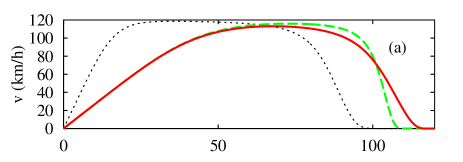
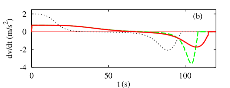
FIG. 2.: Temporal evolution of velocity and acceleration of a single driver-vehicle unit which accelerates on a 2.5 km long stretch of free road before it decelerates when approaching a standing obstacle at $x=2.5$ km. The dynamics for the IDM parameters of Table I (solid) is compared with the result for an increased acceleration $a_{0}=2$ m/s (dotted), or an increased braking deceleration $b=5$ m/s² (dashed).

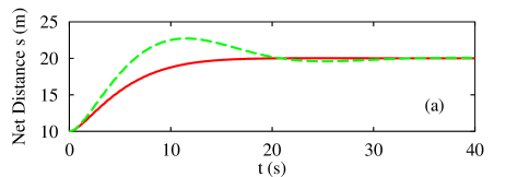
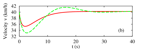
FIG. 3.: Adaptation of a single vehicle to the equilibrium distance in the car-following regime. Shown is (a) the net distance $s$, and (b) the velocity of a vehicle following a queue of vehicles which all drive at $v^{*}=40.5$ km/h corresponding to an equilibrium distance $s_{e}=20$ m. The initial conditions are $v(0)=v^{*}$ and $s(0)=s_{e}/2=10$ m. The solid line is for the IDM standard parameters, and the dashed line for the deceleration parameter $b$ increased from 1.67 m/s² to 10 m/s².

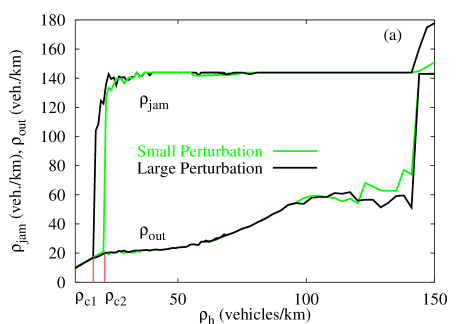
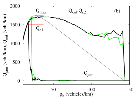
FIG. 4.: Stability diagram of homogeneous traffic on a circular road as a function of the homogeneous density $\rho_{h}$ for small (grey) and large (black) initial perturbations of the density. In plot (a), the upper two lines display the density inside of density clusters after a stationary state has been reached. The lower two lines represent the density between the clusters. Plot (b) shows the corresponding flows and the equilibrium flow-density relation (thin curve). The critical densities $\rho_{{\rm c}i}$ and flows $Q_{{\rm c}i}$ are discussed in the main text. For $\rho_{\rm c2}\leq\rho_{h}\leq 45$ vehicles/km, the outflow $Q_{\rm out}\approx Q_{\rm c2}$ and the corresponding density $\rho_{\rm out}$ are constant. Here, we have $Q_{\rm max}\approx Q_{\rm out}$ for the maximum equilibrium flow, but there are other parameter sets (especially if $s_{1}>0$) where $Q_{\rm max}$ is clearly larger than $Q_{\rm out}$ [37].

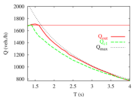
FIG. 5.: Outflow $Q_{\rm out}$ from congested traffic (solid curve), minimum flow $Q_{\rm c1}$ for nonlinear instabilities (dashed), and maximum equilibrium flow $Q_{\rm max}$ (dotted) as a function of the safe time headway. An approximation for the bottleneck strength $\delta Q$ of the phase diagram is given by the difference between the value $Q_{\rm out}=1689$ vehicles/h for $T=1.6$ s (horizontal thin line), and $Q_{\rm out}(T)$. For decerasing values of $T$ traffic becomes more unstable which is indicated by increasing differences ($Q_{\rm max}-Q_{\rm out}$) or ($Q_{\rm max}-Q_{\rm c1}$). For $T\leq 1.5$ s this even leads to $\partial Q_{\rm out}(T)/\partial T>0$. Furthermore, $Q_{\rm out}\approx Q_{\rm c1}$ for $T\leq 1.4$ s.

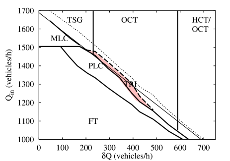
FIG. 6.: Phase diagram resulting from IDM simulations of an open system with a flow-conserving bottleneck. The bottleneck is realized by an increased IDM parameter $T$ in the downstream region, cf. Eq. (16). The control parameters are the traffic flow $Q_{\rm in}$ and the bottleneck strength $\delta Q$, see Eq. (15). The solid thick lines separate the congested traffic states TSG, OCT, HCT, PLC, and MLC (cf. the main text and Fig. 7) and free traffic (FT) as they appear after adiabatically increasing the inflow to the value $Q_{\rm in}$ and applying a large perturbation afterwards (history “C” in the main text). Also shown is the critical downstream flow $Q^{\prime}_{\rm c2}(\delta Q)$ (thin solid line), below which free traffic (FT) is (meta-)stable, and the maximum downstream flow $Q^{\prime}_{\rm max}(\delta Q)$ (thin dotted) below which (possibly unstable) equilibrium traffic exists. Traffic is bistable for inflows above the lines FT-PLC or FT-MLC (whichever is lower), and below $Q^{\prime}_{\rm c2}(\delta Q)$. In the smaller shaded region, traffic is tristable and the possible states FT, PLC, or OCT depend on the previous history (see the main text). For history “C” we obtain OCT in this region.

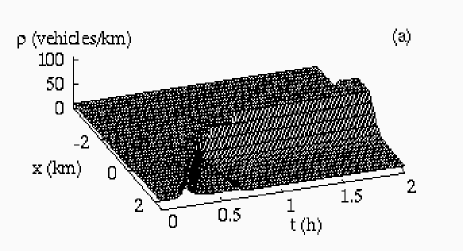
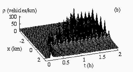
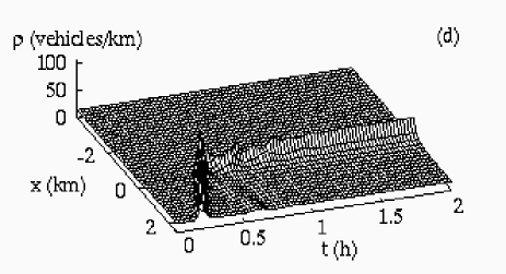
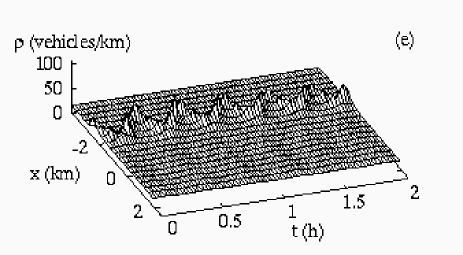
FIG. 7.: Spatio-temporal density plots of the traffic states appearing in the phase diagram of Fig. 6. (a) Homogeneous congested traffic (HCT), (b) oscillating congested traffic (OCT), (c) triggered stop-and-go waves (TSG), (d) (stationary) pinned localized cluster (SPLC), and (e) oscillatory pinned localized cluster (OPLC). The latter two states are summarized as pinned localized clusters (PLC). After a stationary state of free traffic has developed, a density wave is introduced through the downstream boundary (or initial conditions) which eventually triggers the breakdown (History “C”, cf. the main text).

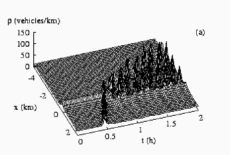
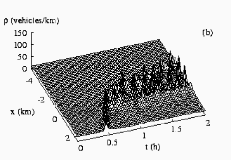
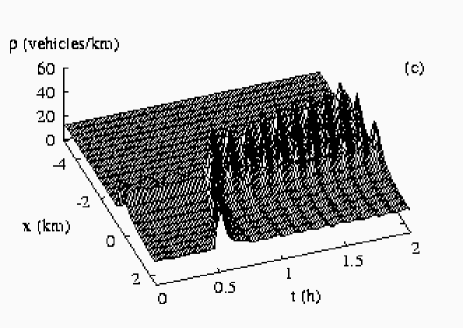
FIG. 8.: Spatio-temporal density plots for the same phase point in the tristable traffic regime, but different histories. (a) Metastable PLC and stable OCT. The system is the same as in Fig. 7 with $Q_{\rm in}=1440$ vehicles/h and $T^{\prime}=1.95$ s ($\delta Q=270$ vehicles/h). The metastable PLC is triggered by a triangular-shaped density peak in the initial conditions (of total width 600 m, centered at $x=0$), in which the density rises from 14 vehicles/km to 45 vehicles km. The OCT is triggered by a density wave introduced by the downstream boundary conditions. (b) Same system as in (a), but starting with metastable free traffic. Here, the transition to OCT is triggered by a density wave coming from the downstream boundary. (c) Similar behavior as in (a), but for the GKT model (with model parameters $v_{0}=120$ km/h, $T=1.8$ s, $\tau=50$ s, $\rho_{\rm max}=130$ vehicles/km, $\gamma=1.2$, $A_{0}=0.008$, and $\Delta A=0.008$, cf. Ref. [27]).

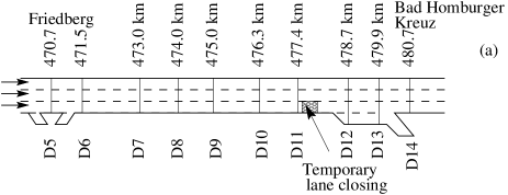
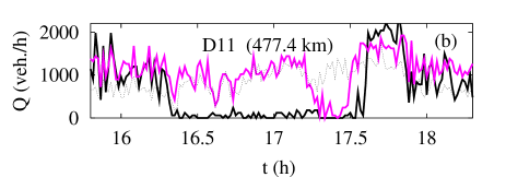
FIG. 9.: Traffic breakdown to nearly homogeneous congested traffic on the freeway A5-South near Frankfurt triggered by a temporary incident between 16:20 and 17:30 on Aug. 6, 1998 between the cross sections D11 and D12. (a) Sketch of the freeway. (b) Flows at cross section D11 on the right lane (solid black), middle lane (grey), and left lane (dotted).

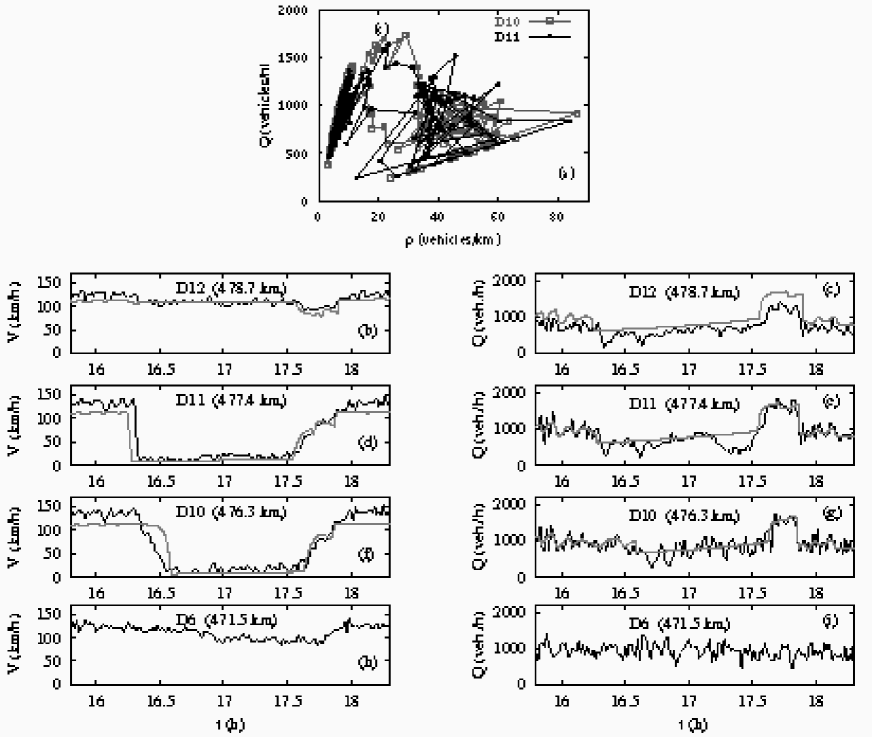
FIG. 10.: [Please display in two columns as indicated] Details of the traffic breakdown depicted in Fig. 9. (a) Flow-density diagram of the traffic breakdown on the A5 South, (b)-(g) temporal evolution of velocity and flow at three locations near the perturbation, and (h), (i) inflow boundary conditions taken from cross section D6. Besides the data (black lines), the results of the microsimulation are shown (grey). All empirical quantities are averages over one minute and over all three lanes.

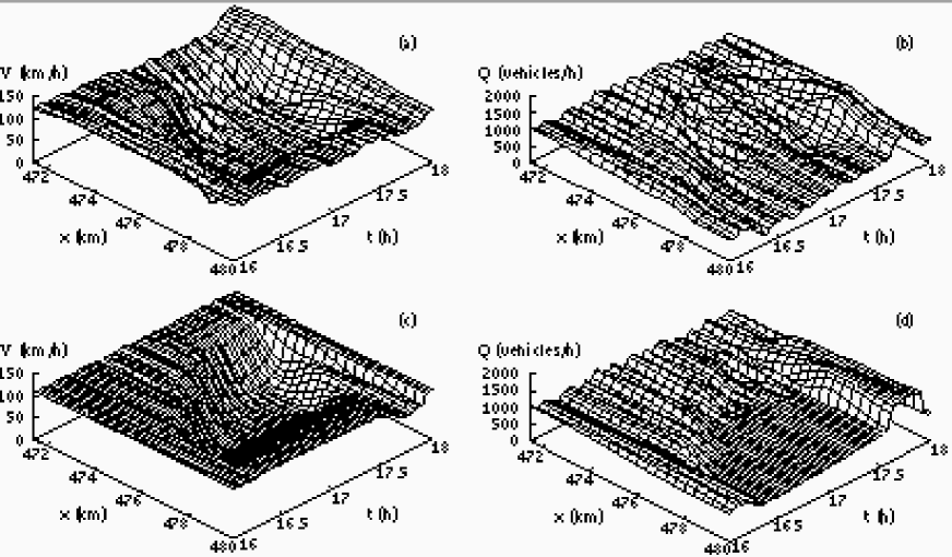
FIG. 11.: [Please display in two columns as indicated] (a), (b) Smoothed spatio-temporal velocity and flow from the data of the traffic breakdown depicted in Figs. 9 and 10. (c), (d) Corresponding IDM microsimulation with the parameter set from Table I. The upstream boundary conditions for velocity and traffic flow were taken from cross section D6. Because of the fast relaxation of the velocity to the model’s equilibrium value, the upstream boundary conditions for the empirical velocity plots (a) seem to be different from the simulation (c) (see main text). Homogeneous von Neumann boundary conditions were assumed downstream. The temporary lane closing is modelled by locally increasing the IDM parameter $T$ in a 1000 m long section centered at $x=478$ km during the time interval 16:20 h $\leq t\leq$ 17:30 h of the incident.

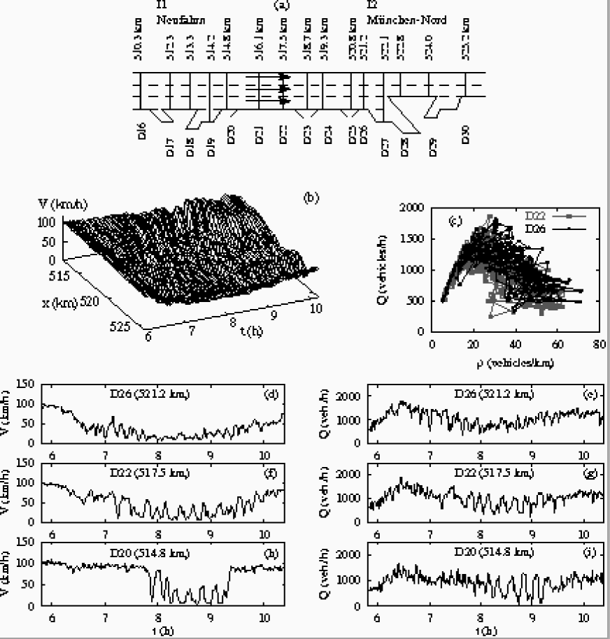
FIG. 12.: [Please display in two columns as indicated] Traffic breakdown to oscillating congested traffic in the evening rush hour of October 29, 1998 on the freeway A9-South near Munich. (a) Sketch of the considered section with the cross sections D16 to D30 and their positions in kilometers. The small on- and off-ramps between I1 and I2, which have been neglected in our simulation, are indicated by diagonal lines. (b) Spatio-temporal plot of the smoothed lane-averaged velocity. (c) Flow-density diagram obtained from two detectors in the congested region. (d)-(i) Lane-averaged 1-minute data of velocities and flows.

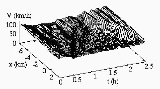
FIG. 13.: Smoothed spatio-temporal velocity plot from a qualitative IDM microsimulation of the situation depicted in Fig. 12. As inflow boundary conditions, we used the traffic flow data of cross section D20. Homogeneous von Neumann boundary conditions were assumed at the downstream boundary. The inhomogeneity was implemented by a local, but time-independent increase of $T$ in the region $x\geq 0$ km from $T=2.2$ s to $T^{\prime}=2.5$ s.

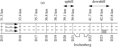
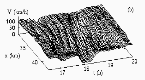
FIG. 14.: Oscillating congested traffic (OCT) on an uphill section of the freeway A8 East (near Munich). (a) Sketch of the section with the cross sections D15 to D24 and their positions in kilometers. (b) Smoothed lane-averaged empirical velocity. An incident leading to a temporary lane closing between D23 and D24 (near the downstream boundaries of the plots) induces even denser congested traffic that propagates through the OCT region. (c) Microsimulation using the data of cross sections D15 and D23 as upstream and downstream boundary conditions, respectively. The uphill section is modelled by linearly increasing the safe time headway from $T=1.6$ s (for $x<39.3$ km) to $T^{\prime}=1.9$ s (for $x>40.0$ km). As in the previous microsimulations, the velocity near the upstram boundary relaxes quickly and, therefore, seems to be inconsistent with the empirical values (see main text).

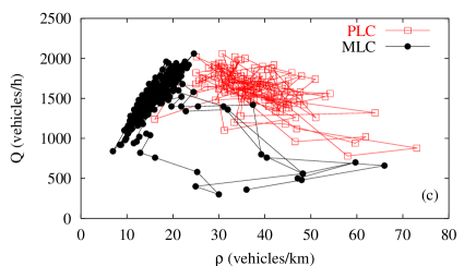
FIG. 15.: Data of two moving localized clusters (MLCs), and pinned localized clusters (PLC) on the freeway A5-North near Frankfurt. (a) Sketch of the infrastructure with the positions of the cross sections D5 - D16 in kilometers. (b) Spatio-temporal plot of the density. (c) Flow-density diagram for detector D6, where there are only stop-and-go waves ($\Box$), and for detector D13 ($\bullet$), where we have omitted data points during the time intervals when the MLCs passed by. (d)-(f) Temporal evolution of the velocity (one-minute data) at the location of the PLC at D13, and upstream (D18) and downstream (D6) of it.

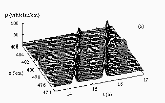
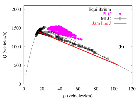
FIG. 16.: Smoothed spatio-temporal plot of the traffic density showing the coexistence of a pinned localized cluster (PLC) with moving localized clusters (MLCs) in an IDM simulation. The PLC is positioned at a road section with locally increased capacity corresponding to a bottleneck strength $\delta Q=-300$ vehicles/h, which can be identified with the region between the off- and on-ramps of intersection I2 in Fig. 15(a). It was produced by locally decreasing the IDM parameter $T$ from 1.9 s to $T^{\prime}=1.6$ s in a 400 m wide section centered at $x=480.8$ km, and increasing it again from $T^{\prime}$ to $T$ in a 400 m wide section centered at $x=480.2$ km. The initial conditions correspond to equilibrium traffic of flow $Q_{\rm in}=1390$ vehicles/h, to which a triangular-shaped density peak (with maximum density 60 vehicles/km at $x=480.5$ km and total width 1 km) was superposed to initialize the PLC. As upstram boundary conditions, we assumed free equilibrium traffic with a constant inflow $Q_{\rm in}$ of 1390 vehicles/h. As downstream boundary conditions for the velocity, we used the value for equilibrium free traffic most of the time. However, for two five-minute intervals at 14:20 h and 15:40 h, we reduced the velocity to $v=12$ km/h to initialize the MLCs. (b) Flow-density diagram of virtual detectors located at the position $x=480.2$ km (PLC), and 2.2 km downstream of it (MLC). Again, the time intervals, where density waves passed through the PLC, were omitted in the (“virtual”) data points belonging to PLC. The thin solid curve indicates the equilibrium flow density relation and the thick solid line $J$ characterizes the outflow from fully developed density clusters to free traffic, cf. Ref. [7], both for $T=1.9$ s.

FIG. 17.: Flow-density diagram of a HCT state of single-lane heterogeneous traffic consisting of 70% “cars” and 30% “trucks”. Trucks are characterized by lower IDM parameters $v_{0}$ and $a$, and a larger $T$ compared to cars. The solid and dashed curves give the equilibrium flow-density relations for traffic consisting only of cars and trucks, respectively. For details, see Ref. [37].

REFERENCES

- [1] F. L. Hall and K. Agyemang-Duah, Transp. Res. Rec. 1320, 91 (1991).
- [2] C. F. Daganzo, in Proceedings of the 13rd International Symbosium on Transportation and Traffic theory, edited by J. B. Lesort (Pergamon, Tarrytown, 1996), p. 629.
- [3] B. S. Kerner and H. Rehborn, Phys. Rev. E 53, R4275 (1996).
- [4] B. S. Kerner and H. Rehborn, Phys. Rev. Lett. 79, 4030 (1997).
- [5] T. Nagatani, J. Phys. Soc. Japan 66, L1928 (1997).
- [6] B. Persaud, S. Yagar, and R. Brownlee, Transportation Research Record 1634, 64 (1998).
- [7] B. S. Kerner, Phys. Rev. Lett. 81, 3797 (1998).
- [8] D. Helbing and M. Treiber, Phys. Rev. Lett. 81, 3042 (1998).
- [9] D. Helbing and M. Treiber, Science 282, 2001 (1998).
- [10] H. Y. Lee, H. W. Lee, and D. Kim, Phys. Rev. Lett. 81, 1130 (1998).
- [11] H. Y. Lee, H. W. Lee, and D. Kim, Phys. Rev. E 59, 5101 (1999).
- [12] H. Y. Lee and H. W. Lee and D. Kim, Empirical Phase Diagram of Congested Traffic Flow, Preprint cond-mat/9905292.
- [13] C. F. Daganzo, M. J. Cassidy, and R. L. Bertini, Transportation Research B 33, 25 (1999).
- [14] D. Helbing, A. Hennecke, and M. Treiber, Phys. Rev. Lett. 82, 4360 (1999).
- [15] B. S. Kerner, Congested traffic flow: Observations and theory, Transportation Research Record 1999, in print.
- [16] B. S. Kerner and H. Rehborn, Internationales Verkehrswesen 5, 196 (1998).
- [17] D. Helbing and M. Treiber, Computing in Science and Engineering (CiSE) 5, 89 (1999).
- [18] D. Helbing, Verkehrsdynamik (Springer, Berlin, 1997).
- [19] D. Helbing, Phys. Rev. E 55, R25 (1997).
- [20] M. Treiber and D. Helbing, J. Phys. A 32, L17 (1999).
- [21] S. Smulders, 7th International Conference on Road Traffic Monitoring and Control (IEE, London, 1994), pp. 145–149.
- [22] V. Shvetsov and D. Helbing, Phys. Rev. E 59, 6328 (1999).
- [23] B. S. Kerner and H. Rehborn, Phys. Rev. E 53, R1297 (1996).
- [24] M. J. Lighthill and G. B. Whitham, Proc. Roy. Soc. of London A 229, 317 (1955).
- [25] M. Cremer and F. Meißner, Traffic Prediction and Optimization Using an Efficient Macroscopic Simulation Tool. In: A. Pave, ed. Modelling and Simulation 1993, pp. 513-519. Society for Computer Simulation International, Ghent, Belgium.
- [26] B. S. Kerner and P. Konhäuser, Phys. Rev. E 50, 54 (1994).
- [27] M. Treiber, A. Hennecke, and D. Helbing, Phys. Rev. E 59, 239 (1999).
- [28] G. F. Newell, Operations Research 9, 209 (1961).
- [29] P. G. Gipps, Transportation Research B 15, 105 (1981).
- [30] R. Wiedemann, Simulation des Straßenverkehrsflusses. Schriftenreihe des IfV, Vol. 8 (Institut für Verkehrswesen, University of Karlsruhe, Germany, 1974).
- [31] M. Bando et al., Phys. Rev. E 51, 1035 (1995).
- [32] S. Krauß, in Traffic and Granular Flow ’97, edited by M. Schreckenberg and D. E. Wolf (Springer, Singapore, 1998), pp. 269–283.
- [33] B. Tilch and D. Helbing, Phys. Rev. E 58, 133 (1998).
-
[34]
For an overview, see the internet page
http://hippo.mit.edu/products/mitsim/main.html. - [35] L. D. Howe, Physica A 246, 157 (1997).
- [36] M. Treiber and D. Helbing, “Explanation of observed features of self-organization in traffic flow”. Preprint cond-mat/9901239.
- [37] M. Treiber, A. Hennecke, and D. Helbing, in Traffic and Granular Flow ’99, edited by D. Helbing, H. J. Herrmann, M. Schreckenberg, and D. E. Wolf (Springer, Berlin, 2000), in print.
- [38] O. Biham, A. A. Middleton, and D. Levine, Phys. Rev. A 46, R6124 (1992).
- [39] M. Cremer and J. Ludwig, Math. Comput. Simulation 28, 297 (1986).
- [40] K. Nagel and M. Schreckenberg, J. Phys. I France 2, 2221 (1992).
- [41] R. Barlovic, L. Santen, A. Schadschneider, and M. Schreckenberg, Traffic and Granular Flow ’97 (Springer, Singapore, 1998), p. 335.
- [42] D. Helbing and B. A. Huberman, Nature 396, 738 (1998).
- [43] D. E. Wolf, Physica A 263, 438 (1999).
- [44] R. D. Kühne, in Proceedings of the 9th International Symposium on Transportation and Traffic Theory, edited by I. Volmuller and R. Hamerslag (VNU Science Press, Utrecht, 1984), p. 21
- [45] J. Treiterer and J. A. Myers, in Proc. 6th Int. Symp. on Transportation and Traffic Theory, edited by D. J. Buckley (Elsevier, New York, 1974), p. 13, empirical observation of trajectories.
- [46] A. Hennecke, M. Treiber, and D. Helbing, in Traffic and Granular Flow ’99, edited by D. Helbing, H. J. Herrmann, M. Schreckenberg, and D. E. Wolf (Springer, Berlin, 2000), p. to be published.
- [47] A. Reuschel, Österreichisches Ingenieur-Archiv 4, 193 (1950).
- [48] R. E. Chandler, R. Herman, and E. W. Montroll, Operations Research 6, 165 (1958).
- [49] R. Herman, E. W. Montroll, R. B. Potts, and R. W. Rothery, Operations Research 7, 86 (1959).
- [50] D. C. Gazis, R. Herman, and R. W. Rothery, Operations Research 9, 545 (1961).
- [51] L. C. Edie, Transp. Res. B 28, 66 (1961).
- [52] T. Bleile, Modellierung des Fahrzeugfolgeverhaltens im innerstädtischen PKW-Verkehr, (Phd thesis, University of Stuttgart, Germany, 1999).
- [53] P. G. Gipps, Transp. Res. 20 B, 403 (1986).
- [54] M. Muramatsu and T. Nagatani, Phys. Rev. E 60, 180 (1999).
- [55] The simulations were performed on a personal workstation with a 433 Mhz Alpha processor.
- [56] B. S. Kerner, P. Konhäuser, and M. Schilke, Phys. Rev. E 51, 6243 (1995).
- [57] Since speed limits lead to reduced desired velocities for many drivers as well, one might conclude that speed limits also cause undesirable local bottlenecks. The main effect of speed limits is, however, to reduce the velocity variance which leads to less braking maneuvers and de facto to a higher capacity. In contrast, gradients mainly influence slow vehicles (trucks), leading to higher values for the velocity variance.
- [58] D. C. Gazis and R. Herman, Transportation Science 26(3),223–229 (1992).
- [59] E. Ben-Naim and P. L. Krapivsky, Phys. Rev. E 56, 6680 (1997).
- [60] Interactive simulations of the multi-lane IDM are available at www.theo2.physik.uni-stuttgart.de/treiber/MicroApplet/.