Foundations of Dissipative Particle Dynamics

Abstract

We derive a mesoscopic modeling and simulation technique that is very close to the technique known as dissipative particle dynamics. The model is derived from molecular dynamics by means of a systematic coarse-graining procedure. This procedure links the forces between the dissipative particles to a hydrodynamic description of the underlying molecular dynamics (MD) particles. In particular, the dissipative particle forces are given directly in terms of the viscosity emergent from MD, while the interparticle energy transfer is similarly given by the heat conductivity derived from MD. In linking the microscopic and mesoscopic descriptions we thus rely on the macroscopic description emergent from MD. Thus the rules governing our new form of dissipative particle dynamics reflect the underlying molecular dynamics; in particular all the underlying conservation laws carry over from the microscopic to the mesoscopic descriptions. We obtain the forces experienced by the dissipative particles together with an approximate form of the associated equilibrium distribution. Whereas previously the dissipative particles were spheres of fixed size and mass, now they are defined as cells on a Voronoi lattice with variable masses and sizes. This Voronoi lattice arises naturally from the coarse-graining procedure which may be applied iteratively and thus represents a form of renormalisation-group mapping. It enables us to select any desired local scale for the mesoscopic description of a given problem. Indeed, the method may be used to deal with situations in which several different length scales are simultaneously present. We compare and contrast this new particulate model with existing continuum fluid dynamics techniques, which rely on a purely macroscopic and phenomenological approach. Simulations carried out with the present scheme show good agreement with theoretical predictions for the equilibrium behavior.

I Introduction

The non-equilibrium behavior of fluids continues to present a major challenge for both theory and numerical simulation. In recent times, there has been growing interest in the study of so-called ‘mesoscale’ modeling and simulation methods, particularly for the description of the complex dynamical behavior of many kinds of soft condensed matter, whose properties have thwarted more conventional approaches. As an example, consider the case of complex fluids with many coexisting length and time scales, for which hydrodynamic descriptions are unknown and may not even exist. These kinds of fluids include multi-phase flows, particulate and colloidal suspensions, polymers, and amphiphilic fluids, including emulsions and microemulsions. Fluctuations and Brownian motion are often key features controlling their behavior.

From the standpoint of traditional fluid dynamics, a general problem in describing such fluids is the lack of adequate continuum models. Such descriptions, which are usually based on simple conservation laws, approach the physical description from the macroscopic side, that is in a ‘top down’ manner, and have certainly proved successful for simple Newtonian fluids [1]. For complex fluids, however, equivalent phenomenological representations are usually unavailable and instead it is necessary to base the modeling approach on a microscopic (that is on a particulate) description of the system, thus working from the bottom upwards, along the general lines of the program for statistical mechanics pioneered by Boltzmann [2]. Molecular dynamics (MD) presents itself as the most accurate and fundamental method [3] but it is far too computationally intensive to provide a practical option for most hydrodynamic problems involving complex fluids. Over the last decade several alternative ‘bottom up’ strategies have therefore been introduced. Hydrodynamic lattice gases [4], which model the fluid as a discrete set of particles, represent a computationally efficient spatial and temporal discretization of the more conventional molecular dynamics. The lattice-Boltzmann method [5], originally derived from the lattice-gas paradigm by invoking Boltzmann’s Stosszahlansatz, represents an intermediate (fluctuationless) approach between the top-down (continuum) and bottom-up (particulate) strategies, insofar as the basic entity in such models is a single particle distribution function; but for interacting systems even these lattice-Boltzmann methods can be subdivided into bottom-up [6] and top-down models [7].

A recent contribution to the family of bottom-up approaches is the dissipative particle dynamics (DPD) method introduced by Hoogerbrugge and Koelman in 1992 [8]. Although in the original formulation of DPD time was discrete and space continuous, a more recent re-interpretation asserts that this model is in fact a finite-difference approximation to the ‘true’ DPD, which is defined by a set of continuous time Langevin equations with momentum conservation between the dissipative particles [9]. Successful applications of the technique have been made to colloidal suspensions [10], polymer solutions [11] and binary immiscible fluids [12]. For specific applications where comparison is possible, this algorithm is orders of magnitude faster than MD [13]. The basic elements of the DPD scheme are particles that represent rather ill-defined ‘mesoscopic’ quantities of the underlying molecular fluid. These dissipative particles are stipulated to evolve in the same way that MD particles do, but with different inter-particle forces: since the DPD particles are pictured to have internal degrees of freedom, the forces between them have both a fluctuating and a dissipative component in addition to the conservative forces that are present at the MD level. Newton’s third law is still satisfied, however, and consequently momentum conservation together with mass conservation produce hydrodynamic behavior at the macroscopic level.

Dissipative particle dynamics has been shown to produce the correct macroscopic (continuum) theory; that is, for a one-component DPD fluid, the Navier-Stokes equations emerge in the large scale limit, and the fluid viscosity can be computed [14, 15]. However, even though dissipative particles have generally been viewed as clusters of molecules, no attempt has been made to link DPD to the underlying microscopic dynamics, and DPD thus remains a foundationless algorithm, as is that of the hydrodynamic lattice gas and a fortiori the lattice-Boltzmann method. It is the principal purpose of the present paper to provide an atomistic foundation for dissipative particle dynamics. Among the numerous benefits gained by achieving this, we are then able to provide a precise definition of the term ‘mesoscale’, to relate the hitherto purely phenomenological parameters in the algorithm to underlying molecular interactions, and thereby to formulate DPD simulations for specific physicochemical systems, defined in terms of their molecular constituents. The DPD that we derive is a representation of the underlying MD. Consequently, to the extent that the approximations made are valid, the DPD and MD will have the same hydrodynamic descriptions, and no separate kinetic theory for, say, the DPD viscosity will be needed once it is known for the MD system. Since the MD degrees of freedom will be integrated out in our approach the MD viscosity will appear in the DPD model as a parameter that may be tuned freely.

In our approach, the ‘dissipative particles’ (DP) are defined in terms of appropriate weight functions that sample portions of the underlying conservative MD particles, and the forces between the dissipative particles are obtained from the hydrodynamic description of the MD system: the microscopic conservation laws carry over directly to the DPD, and the hydrodynamic behavior of MD is thus reproduced by the DPD, albeit at a coarser scale. The mesoscopic (coarse-grained) scale of the DPD can be precisely specified in terms of the MD interactions. The size of the dissipative particles, as specified by the number of MD particles within them, furnishes the meaning of the term ‘mesoscopic’ in the present context. Since this size is a freely tunable parameter of the model, the resulting DPD introduces a general procedure for simulating microscopic systems at any convenient scale of coarse graining, provided that the forces between the dissipative particles are known. When a hydrodynamic description of the underlying particles can be found, these forces follow directly; in cases where this is not possible, the forces between dissipative particles must be supplemented with the additional components of the physical description that enter on the mesoscopic level.

The DPD model which we derive from molecular dynamics is formally similar to conventional, albeit foundationless, DPD [14]. The interactions are pairwise and conserve mass and momentum, as well as energy [16, 17]. Just as the forces conventionally used to define DPD have conservative, dissipative and fluctuating components, so too do the forces in the present case. In the present model, the role of the conservative force is played by the pressure forces. However, while conventional dissipative particles possess spherical symmetry and experience interactions mediated by purely central forces, our dissipative particles are defined as space-filling cells on a Voronoi lattice whose forces have both central and tangential components. These features are shared with a model studied by Español [18]. This model links DPD to smoothed particle hydrodynamics [19] and defines the DPD forces by hydrodynamic considerations in a way analogous to earlier DPD models. Español et al. [20] have also carried out MD simulations with a superposed Voronoi mesh in order to measure the coarse grained inter-DP forces.

While conventional DPD defines dissipative particle masses to be constant, this feature is not preserved in our new model. In our first publication on this theory [21], we stated that, while the dissipative particle masses fluctuate due to the motion of MD particles across their boundaries, the average masses should be constant. In fact, the DP-masses vary due to distortions of the Voronoi cells, and this feature is now properly incorporated in the model.

We follow two distinct routes to obtain the fluctuation-dissipation relations that give the magnitude of the thermal forces. The first route follows the conventional path which makes use of a Fokker-Planck equation [9]. We show that the DPD system is described in an approximate sense by the isothermal-isobaric ensemble. The second route is based on the theory of fluctuating hydrodynamics and it is argued that this approach corresponds to the statistical mechanics of the grand canonical ensemble. Both routes lead to the same result for the fluctuating forces and simulations confirm that, with the use of these forces, the measured DP temperature is equal to the MD temperature which is provided as input. This is an important finding in the present context as the most significant approximations we have made underlie the derivation of the thermal forces.

II Coarse-graining molecular dynamics: from micro to mesoscale

The essential idea motivating our definition of mesoscopic dissipative particles is to specify them as clusters of MD particles in such a way that the MD particles themselves remain unaffected while all being represented by the dissipative particles. The independence of the molecular dynamics from the superimposed coarse-grained dissipative particle dynamics implies that the MD particles are able to move between the dissipative particles. The stipulation that all MD particles must be fully represented by the DP’s implies that while the mass, momentum and energy of a single MD particle may be shared between DP’s, the sum of the shared components must always equal the mass and momentum of the MD particle.

A Definitions

Full representation of all the MD particles can be achieved in a general way by introducing a sampling function

$$f_{k}({\bf x})=\frac{s({\bf x}-{\bf r}_{k})}{\sum_{l}s({\bf x}-{\bf r}_{l})}\;.$$ (1)

where the positions ${\bf r}_{k}$ and ${\bf r}_{l}$ define the DP centers, ${\bf x}$ is an arbitrary position and $s({\bf x})$ is some localized function. It will prove convenient to choose it as a Gaussian

$$s({\bf x})=\exp{(-x^{2}/a^{2})}$$ (2)

where the distance $a$ sets the scale of the sampling function, although this choice is not necessary. The mass, momentum and internal energy $E$ of the $k$th DP are then defined as

$$M_{k} = \sum_{i}f_{k}({\bf x}_{i})m,$$ (3)

$${\bf P}_{k} = \sum_{i}f_{k}({\bf x}_{i})m{\bf v}_{i},$$ (4)

$$\frac{1}{2}M_{k}U_{k}^{2}+E_{k} = \sum_{i}f_{k}({\bf x}_{i})\left(\frac{1}{2}mv_{i}^{2}+\frac{1}{2}\sum_{j\neq i}V_{MD}(r_{ij})\right)$$ (5)

$$\equiv \sum_{i}f_{k}({\bf x}_{i})\epsilon_{i},$$ (6)

where ${\bf x}_{i}$ and ${\bf v}_{i}$ are the position and velocity of the $i$th MD particle, which are all assumed to have identical masses $m$, ${\bf P}_{k}$ is the momentum of the $k$th DP and $V_{MD}(r_{ij})$ is the potential energy of the MD particle pair $ij$, separated a distance $r_{ij}$. The particle energy $\epsilon_{i}$ thus contains both the kinetic and a potential term. The kinematic condition

$$\dot{{\bf r}}_{k}={\bf U}_{k}\equiv{\bf P}_{k}/M_{k}$$ (7)

completes the definition of our dissipative particle dynamics.

It is generally true that mass and momentum conservation suffice to produce hydrodynamic behavior. However, the equations expressing these conservation laws contain the fluid pressure. In order to get the fluid pressure a thermodynamic description of the system is needed. This produces an equation of state, which closes the system of hydrodynamic equations. Any thermodynamic potential may be used to obtain the equation of state. In the present case we shall take this potential to be the internal energy $E_{k}$ of the dissipative particles, and we shall obtain the equations of motion for the DP mass, momentum and energy. Note that the internal energy would also have to be computed if a free energy had been chosen for the thermodynamic description. For this reason it is not possible to complete the hydrodynamic description without taking the energy flow into account. As a byproduct of this the present DPD also contains a description of the heat flow and corresponds to the recently introduced DPD with energy conservation [16, 17]. Español previously introduced an angular momentum variable describing the dynamics of extended particles [18]: this is needed when forces are non-central in order to avoid dissipation of energy in a rigid rotation of the fluid. Angular momentum could be included on the same footing as momentum in the following developments. However for reasons both of space and conceptual economy we shall omit it in the present context, even though it is probably important in applications where hydrodynamic precision is important. In the following sections, we shall use the notation ${\bf r}$, $M$, ${\bf P}$ and $E$ with the indices $k\;,l\;,m$ and $n$ to denote DP’s while we shall use ${\bf x}$, $m$, ${\bf v}$ and $\epsilon$ with the indices $i$ and $j$ to denote MD particles.

B Equations of motion for the dissipative particles based on a microscopic description

The fact that all the MD particles are represented at all instants in the coarse-grained scheme is guaranteed by the normalization condition $\sum_{k}f_{k}({\bf x})=1$. This implies directly that

$$\sum_{k}M_{k} = \sum_{i}m$$ (8)

$$\sum_{k}{\bf P}_{k} = \sum_{i}m{\bf v}_{i}$$ (9)

$$\sum_{k}E_{k}^{\text{tot}} = \sum_{k}\left(\frac{1}{2}M_{k}{\bf U}_{k}^{2}+E_{k}\right)=\sum_{i}\epsilon_{i}\;;$$ (10)

thus with mass, momentum and energy conserved at the MD level, these quantities are also conserved at the DP level. In order to derive the equations of motion for dissipative particle dynamics we now take the time derivatives of Eqs. (6). This gives

$$\frac{\text{d}{M_{k}}}{\text{d}t} = \sum_{i}\dot{f}_{k}({\bf x}_{i})m$$ (11)

$$\frac{\text{d}{\bf P}_{k}}{\text{d}t} = \sum_{i}\left(\dot{f}_{k}({\bf x}_{i})m{\bf v}_{i}+{f}_{k}({\bf x}_{i}){\bf F}_{i}\right)$$ (12)

$$\frac{\text{d}E_{k}^{\text{tot}}}{\text{d}t} = \sum_{i}\left(\dot{f}_{k}({\bf x}_{i})\epsilon_{i}+{f}_{k}({\bf x}_{i})\dot{\epsilon}_{i}\right)$$ (13)

where $\text{d}/\text{d}t$ is the substantial derivative and ${\bf F}_{i}=m\dot{{\bf v}}_{i}$ is the force on particle $i$.

The Gaussian form of $s$ implies that
$\dot{s}({\bf x})=-(2/a^{2})\dot{{\bf x}}\cdot{\bf x}s({\bf x})$. This makes it possible to write

$$\dot{f}_{k}({\bf x}_{i})=f_{kl}({\bf x}_{i})({\bf v}^{\prime}_{i}\cdot{\bf r}_{kl}+{\bf x}^{\prime}_{i}\cdot{\bf U}_{kl})$$ (14)

where the overlap function $f_{kl}$ is defined as $f_{kl}({\bf x})\equiv(2/a^{2})f_{k}({\bf x})f_{l}({\bf x})$, ${\bf r}_{kl}\equiv({\bf r}_{k}-{\bf r}_{l})$ and ${\bf U}_{kl}\equiv({\bf U}_{k}-{\bf U}_{l})$, and we have rearranged terms so as to get them in terms of the centered variables

$${\bf v}^{\prime}_{i} = {\bf v}_{i}-\frac{({\bf U}_{k}+{\bf U}_{l})}{2}$$ (15)

$${\bf x}^{\prime}_{i} = {\bf x}_{i}-\frac{({\bf r}_{k}+{\bf r}_{l})}{2}\;.$$ (16)

Before we proceed with the derivation of the equations of motion it is instructive to work out the actual forms of $f_{k}({\bf x})$ and $f_{kl}({\bf x})$ in the case of only two particles $k$ and $l$. Using the Gaussian choice of $s$ we immediately get

$$f_{k}({\bf x})=\frac{1}{1+\left[\exp{(({\bf x}-({\bf r}_{k}+{\bf r}_{l})/2)\cdot({\bf r}_{kl})/(a^{2}))}\right]^{2}}\;.$$ (17)

The overlap function similarly follows:

$$f_{kl}({\bf x})=\frac{1}{2a^{2}}\cosh^{-2}{\left(\left({\bf x}-\frac{{\bf r}_{k}+{\bf r}_{l}}{2}\right)\cdot\left(\frac{{\bf r}_{kl}}{a^{2}}\right)\right)}\;.$$ (18)

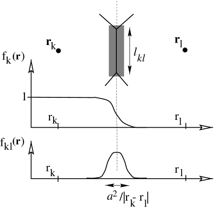
FIG. 1.: The overlap region between two Voronoi cells is shown in grey. The sampling function $f_{k}({\bf r})$ is shown in the top graph and the overlap function $f_{kl}({\bf r})=(2/a^{2})f_{k}({\bf r})f_{l}({\bf r})$ in the bottom graph. The width of the overlap region is $a^{2}/|{\bf r}_{k}-{\bf r}_{l}|$ and its length is denoted by $l$.

These two functions are shown in Fig.1. Note that the scale of the overlap region is not $a$ but $a^{2}/|{\bf r}_{k}-{\bf r}_{l}|$. Dissipative particle interactions only take place where the overlap function is non-zero. This happens along the dividing line which is equally far from the two particles. The contours of non-zero $f_{kl}$ thus define a Voronoi lattice with lattice segments of length $l_{kl}$. This Voronoi construction is shown in Fig. 2 in which MD particles in the overlap region defined by $f_{kl}>0.1$, are shown, though presently not actually simulated as dynamic entities. The volume of the Voronoi cells will in general vary under the dynamics. However, even with arbitrary dissipative particle motion the cell volumes will approach zero only exceptionally, and even then the identities of the DP particles will be preserved so that they subsequently re-emerge.

1 Mass equation

The mass equation (11) takes the form

$$\frac{\text{d}{M_{k}}}{\text{d}t}\equiv\sum_{l}\dot{M}_{kl}$$ (19)

where

$$\dot{M}_{kl}=\sum_{i}{f}_{kl}({\bf x}_{i})m({\bf v}_{i}^{\prime}\cdot{\bf r}_{kl}+{\bf x}^{\prime}_{i}\cdot{\bf U}_{kl})\;.$$ (20)

The ${\bf v}^{\prime}_{i}$ term will be shown to be negligible within our approximations. The ${\bf x}^{\prime}_{i}\cdot{\bf U}_{kl}$-term however describes the geometric effect that the Voronoi cells do not conserve their volume: The relative motion of the DP centers causes the cell boundaries to change their orientation. We will return to give this ‘boundary twisting’ term a quantitative content when the equations of motion are averaged–an effect which was overlooked in our first publication of this theory [21] where it was stated that $\langle\dot{M}_{kl}\rangle=0$.

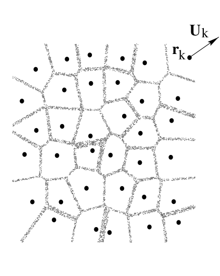
FIG. 2.: The Voronoi lattice defined by the dissipative particle positions ${\bf r}_{k}$. The grey dots which represent the underlying MD particles are drawn only in the overlap region.

2 Momentum equation

The momentum equation (12) takes the form

$$\frac{\text{d}{\bf P}_{k}}{\text{d}t} = \sum_{li}{f}_{kl}({\bf x}_{i})m{\bf v}_{i}({\bf v}_{i}^{\prime}\cdot{\bf r}_{kl}+{\bf x}^{\prime}_{i}\cdot{\bf U}_{kl})$$ (21)

$$+ \sum_{li}f_{k}({\bf x}_{i}){\bf F}_{i}$$ (22)

We can write the force as ${\bf F}_{i}=m{\bf g}+\sum_{j}{\bf F}_{ij}$ where the first term is an external force and the second term is the internal force caused by all the other particles. Newton’s third law then takes the form ${\bf F}_{ij}=-{\bf F}_{ji}$. The last term in Eq. (22) may then be rewritten as

$$\sum_{i}f_{k}({\bf x}_{i}){\bf F}_{i}=M_{k}{\bf g}+\sum_{ij}f_{k}({\bf x}_{i}){\bf F}_{ij}$$ (23)

where

$$\sum_{ij}f_{k}({\bf x}_{i}){\bf F}_{ij} = -\sum_{ij}f_{k}({\bf x}_{i}){\bf F}_{ji}$$ (24)

$$= -\sum_{ij}f_{k}({\bf x}_{j}+\Delta{\bf x}_{ij}){\bf F}_{ji}$$ (25)

$$\approx -\sum_{ij}f_{k}({\bf x}_{j}){\bf F}_{ji}-\sum_{ij}\left(\Delta{\bf x}_{ij}\cdot\nabla f_{k}({\bf x}_{i})\right){\bf F}_{ji}$$ (26)

$$= -\frac{1}{2}\sum_{ij}\left(\Delta{\bf x}_{ij}\cdot\nabla f_{k}({\bf x}_{i})\right){\bf F}_{ji}$$ (27)

$$= \sum_{l}\left\{\sum_{ij}\frac{1}{2}f_{kl}({\bf x}_{i}){\bf F}_{ij}\Delta{\bf x}_{ij}\right\}\cdot{\bf r}_{kl}$$ (28)

where $\Delta{\bf x}_{ij}={\bf x}_{i}-{\bf x}_{j}$, we have Taylor expanded $f_{k}({\bf x})$ around ${\bf x}_{j}$ and used a result similar to Eq. (14) to evaluate $\nabla f_{k}({\bf x})$. In passing from the third to the fourth line in the above equations we have moved the first term on the right hand side to the left hand side and divided by two. Now, if we group the last term above with the ${\bf r}_{kl}$ term in Eq. (22), make use of Eq. (16), and do some rearranging of terms we get

$$\frac{\text{d}{\bf P}_{k}}{\text{d}t} = M_{k}{\bf g}+\sum_{l}\dot{M}_{kl}\frac{{\bf U}_{k}+{\bf U}_{l}}{2}$$ (29)

$$+ \sum_{li}f_{kl}({\bf x}_{i}){\bf\Pi}_{i}^{\prime}\cdot{\bf r}_{kl}$$ (30)

$$+ \sum_{li}f_{kl}({\bf x}_{i})m{\bf v}_{i}^{\prime}{\bf x}_{i}^{\prime}\cdot{\bf U}_{kl}$$ (31)

where we have used the relation $\dot{M}_{k}=\sum_{l}\dot{M}_{kl}$ and defined the general momentum-flux tensor

$${\bf\Pi}_{i}=m{\bf v}_{i}{\bf v}_{i}+\frac{1}{2}\sum_{j}{\bf F}_{ij}\Delta{\bf x}_{ij}\;.$$ (32)

This tensor is the momentum analogue of the mass-flux vector $m{\bf v}_{i}$. The prime indicates that the velocities on the right hand side are those defined in Eq. (16). The tensor ${\bf\Pi}_{i}$ describes both the momentum that the particle carries around through its own motion and the momentum exchanged by inter-particle forces. It may be arrived at by considering the momentum transport across imaginary cross sections of the volume in which the particle is located.

3 Energy equation

In order to get the microscopic energy equation of motion we proceed as with the mass and momentum equations and the two terms that appear on the right hand side of Eq. (13).

Taking $V_{MD}$ to be a central potential and using the relations $\nabla V_{MD}(r_{ij})=V_{MD}^{\prime}(r_{ij}){\bf e}_{ij}=-{\bf F}_{ij}$ and $\dot{V}_{MD}(r_{ij})=V_{MD}^{\prime}(r_{ij}){\bf e}_{ij}\cdot{\bf v}_{ij}=-{\bf F}_{ij}\cdot{\bf v}_{ij}$ where ${\bf v}_{ij}={\bf v}_{i}-{\bf v}_{j}$ we get the time rate of change of the particle energy

$$\dot{\epsilon_{i}}=m{\bf g}\cdot{\bf v}_{i}+\frac{1}{2}\sum_{j\neq i}{\bf F}_{ij}\cdot({\bf v}_{i}+{\bf v}_{j})\;.$$ (33)

This gives the first term of Eq. (13) in the form

$$\sum_{i}f_{k}({\bf x}_{i})\dot{\epsilon}={\bf P}_{k}\cdot{\bf g}+\frac{1}{2}\sum_{i\neq j}f_{k}({\bf x}_{i}){\bf F}_{ij}\cdot({\bf v}_{i}+{\bf v}_{j})\;.$$ (34)

The last term of this equation is odd under the exchange $i\leftrightarrow j$ and exactly the same manipulations as in Eq. (28) may be used to give

$$\sum_{i}f_{k}({\bf x}_{i})\dot{\epsilon} = {\bf P}_{k}\cdot{\bf g}$$ (35)

$$+ \sum_{l,i\neq j}f_{kl}({\bf x}_{i})\frac{1}{4}{\bf F}_{ij}\cdot({\bf v}_{i}+{\bf v}_{j})\Delta{\bf x}_{ij}\cdot{\bf r}_{kl}$$ (36)

$$= {\bf P}_{k}\cdot{\bf g}+\sum_{l,i\neq j}f_{kl}({\bf x}_{i})\left(\frac{1}{4}{\bf F}_{ij}\cdot({\bf v}^{\prime}_{i}+{\bf v}^{\prime}_{j})\right.$$ (37)

$$+ \left.\frac{1}{2}{\bf F}_{ij}\cdot\frac{{\bf U}_{k}+{\bf U}_{l}}{2}\right)\Delta{\bf x}_{ij}\cdot{\bf r}_{kl}$$ (38)

where for later purposes we have used Eqs. (16) to get the last equation. The last term of Eq. (13) is easily written down using Eq. (14). This gives

$$\sum_{i}\dot{f}_{k}({\bf x}_{i})\epsilon_{i}=\sum_{li}f_{kl}({\bf x}_{i})({\bf v}^{\prime}_{i}\cdot{\bf r}_{kl}+{\bf x}^{\prime}_{i}\cdot{\bf U}_{kl})\epsilon_{i}\;.$$ (39)

As previously we write the particle velocities in terms of ${\bf v}_{i}^{\prime}$. The corresponding expression for the particle energy is $\epsilon_{i}=\epsilon^{\prime}_{i}+m{\bf v}_{i}^{\prime}\cdot({\bf U}_{k}+{\bf U}_{l})/2+(1/2)m(({\bf U}_{k}+{\bf U}_{l})/2)^{2}$ where the prime in $\epsilon^{\prime}_{i}$ denotes that the particle velocity is ${\bf v}^{\prime}_{i}$ rather than ${\bf v}_{i}$. Equation (39) may then be written

$$\sum_{i}\dot{f}_{k}({\bf x}_{i})\epsilon_{i} = \sum_{l}\frac{1}{2}\dot{M}_{kl}\left(\frac{{\bf U}_{k}+{\bf U}_{l}}{2}\right)^{2}$$ (40)

$$+ \sum_{li}f_{kl}({\bf x}_{i})\left(\epsilon^{\prime}_{i}{\bf v}_{i}^{\prime}+m{\bf v}_{i}^{\prime}{\bf v}_{i}^{\prime}\cdot\frac{{\bf U}_{k}+{\bf U}_{l}}{2}\right)\cdot{\bf r}_{kl}$$ (41)

$$+ \sum_{li}f_{kl}({\bf x}_{i})\epsilon_{i}{\bf x}^{\prime}_{i}\cdot{\bf U}_{kl}\;.$$ (42)

Combining this equation with Eq. (38) we obtain

$$\dot{E}_{k}^{\text{tot}} = \sum_{li}f_{kl}({\bf x}_{i})\left({\bf J}_{\epsilon i}^{\prime}+\Pi^{\prime}_{i}\cdot\frac{{\bf U}_{k}+{\bf U}_{l}}{2}\right)\cdot{\bf r}_{kl}$$ (43)

$$+ M_{k}{\bf U}_{k}\cdot{\bf g}+\sum_{l}\frac{1}{2}\dot{M}_{kl}\left(\frac{{\bf U}_{k}+{\bf U}_{l}}{2}\right)^{2}$$ (44)

$$+ \sum_{li}f_{kl}({\bf x}_{i})\left(\epsilon^{\prime}_{i}+m{\bf v}^{\prime}_{i}\cdot\left(\frac{{\bf U}_{k}+{\bf U}_{l}}{2}\right)\right){\bf x}^{\prime}_{i}\cdot{\bf U}_{kl}\;.$$ (45)

where the momentum-flux tensor is defined in Eq. (32) and we have identified the energy-flux vector associated with a particle $i$

$${\bf J}_{\epsilon i}=\epsilon_{i}{\bf v}_{i}+\frac{1}{4}\sum_{i\neq j}{\bf F}_{ij}\cdot({\bf v}_{i}+{\bf v}_{j})\Delta{\bf x}_{ij}\;.$$ (46)

Again the prime denotes that the velocities are ${\bf v}^{\prime}_{i}$ rather than ${\bf v}_{i}$. To get the internal energy $\dot{E}_{k}$ instead of $\dot{E}_{k}^{\text{tot}}$ we note that $\text{d}({\bf P}^{2}_{k}/2M_{k})/\text{d}t={\bf U}_{k}\cdot\dot{{\bf P}}_{k}-(1/2)\dot{M}_{k}{\bf U}^{2}_{k}$. Using this relation, the momentum equation Eq. (31), as well as the substitution $({\bf U}_{k}+{\bf U}_{l})/2={\bf U}_{k}-{\bf U}_{kl}/2$ in Eq. (45), followed by some rearrangement of the $\dot{M}_{kl}$ terms we find that

$$\dot{E}_{k}^{\text{tot}} = \frac{\text{d}}{\text{d}t}\left(\frac{1}{2}M_{k}{\bf U}_{k}^{2}\right)$$ (47)

$$+ \sum_{l}\frac{1}{2}\dot{M}_{kl}\left(\frac{{\bf U}_{kl}}{2}\right)^{2}+\sum_{li}f_{kl}({\bf x}_{i})\left({\bf J}_{\epsilon i}^{\prime}-\Pi^{\prime}_{i}\cdot\frac{{\bf U}_{kl}}{2}\right)\cdot{\bf r}_{kl}$$ (48)

$$+ \sum_{li}f_{kl}({\bf x}_{i})\left(\epsilon^{\prime}_{i}-m{\bf v}^{\prime}_{i}\cdot\frac{{\bf U}_{kl}}{2}\right){\bf x}^{\prime}_{i}\cdot{\bf U}_{kl}\;.$$ (49)

This equation has a natural physical interpretation. The first term represents the translational kinetic energy of the DP as a whole. The remaining terms represent the internal energy $E_{k}$. This is a purely thermodynamic quantity which cannot depend on the overall velocity of the DP, i.e. it must be Galilean invariant. This is easily checked as the relevant terms all depend on velocity differences only.

The $\dot{M}_{kl}$ term represents the kinetic energy received through mass exchange with neighboring DPs. As will become evident when we turn to the averaged description, the term involving the momentum and energy fluxes represents the work done on the DP by its neighbors and the heat conducted from them. The $\epsilon^{\prime}_{i}$-term represents the energy received by the DP due to the same ‘boundary twisting’ effect that was found in the mass equation. Upon averaging, the last term proportional to ${\bf v}_{i}^{\prime}$ will be shown to be relatively small since $\langle{\bf v}^{\prime}_{i}\rangle=0$ in our approximations. This is true also in the mass and momentum equations. Equations (20), (31) and (49) have the coarse grained form that will remain in the final DPD equations. Note, however, that they retain the full microscopic information about the MD system, and for that reason they are time-reversible. Equation (31) for instance contains only terms of even order in the velocity. In the next section terms of odd order will appear when this equation is averaged.

It can be seen that the rate of change of momentum in Eq. (31) is given as a sum of separate pairwise contributions from the other particles, and that these terms are all odd under the exchange $l\leftrightarrow k$. Thus the particles interact in a pairwise fashion and individually fulfill Newton’s third law; in other words, momentum conservation is again explicitly upheld. The same symmetries hold for the mass conservation equation (20) and energy equation (45).

III Derivation of dissipative particle dynamics: average and fluctuating forces

We can now investigate the average and fluctuating parts of Eqs. (49), (31) and (20). In so doing we shall need to draw on a hydrodynamic description of the underlying molecular dynamics and construct a statistical mechanical description of our dissipative particle dynamics. For concreteness we shall take the hydrodynamic description of the MD system in question to be that of a simple Newtonian fluid [1]. This is known to be a good description for MD fluids based on Lennard-Jones or hard sphere potentials, particularly in three dimensions [3]. Here we shall carry out the analysis for systems in two spatial dimensions; the generalization to three dimensions is straight forward, the main difference being of a practical nature as the Voronoi construction becomes more involved.

We shall begin by specifying a scale separation between the dissipative particles and the molecular dynamics particles by assuming that

$${|{\bf x}_{i}-{\bf x}_{j}|}<<{|{\bf r}_{k}-{\bf r}_{l}|}\;,$$ (50)

where ${\bf x}_{i}$ and ${\bf x}_{j}$ denote the positions of neighbouring MD particles. Such a scale separation is in general necessary in order for the coarse-graining procedure to be physically meaningful. Although for the most part in this paper we are thinking of the molecular interactions as being mediated by short-range forces such as those of Lennard-Jones type, a local description of the interactions will still be valid for the case of long-range Coulomb interactions in an electrostatically neutral system, provided that the screening length is shorter than the width of the overlap region between the dissipative particles. Indeed, as we shall show here, the result of doing a local averaging is that the original Newtonian equations of motion for the MD system become a set of Langevin equations for the dissipative particle dynamics. These Langevin equations admit an associated Fokker-Planck equation. An associated fluctuation-dissipation relation relates the amplitude of the Langevin force to the temperature and damping in the system.

A Definition of ensemble averages

With the mesoscopic variables now available, we need to define the correct average corresponding to a dynamical state of the system. Many MD configurations are consistent with a given value of the set $\{{\bf r}_{k},M_{k},{\bf U}_{k},E_{k}\}$, and averages are computed by means of an ensemble of systems with common instantaneous values of the set $\{{\bf r}_{k},M_{k},{\bf U}_{k},E_{k}\}$. This means that only the time derivatives of the set $\{{\bf r}_{k},M_{k},{\bf U}_{k},E_{k}\}$, i.e. the forces, have a fluctuating part. In the end of our development approximate distributions for ${\bf U}_{k}$’s and $E_{k}$’s will follow from the derived Fokker-Planck equations. These distributions refer to the larger equilibrium ensemble that contains all fluctuations in $\{{\bf r}_{k},M_{k},{\bf U}_{k},E_{k}\}$.

It is necessary, to compute the average MD particle velocity $\langle{\bf v}\rangle$ between dissipative particle centers, given $\{{\bf r}_{k},M_{k},{\bf U}_{k},E_{k}\}$. This velocity depends on all neighboring dissipative particle velocities. However, for simplicity we shall only employ a “nearest neighbor” approximation, which consists in assuming that $\langle{\bf v}\rangle$ interpolates linearly between the two nearest dissipative particles. This approximation is of the same nature as the approximation used in the Newtonian fluid stress–strain relation which is linear in the velocity gradient. This implies that in the overlap region between dissipative particles $k$ and $l$

$$\langle{\bf v}^{\prime}\rangle=\langle{\bf v}^{\prime}\rangle({\bf x})=\frac{{\bf x}^{\prime}\cdot{\bf r}_{kl}}{r_{kl}^{2}}{\bf U}_{kl}\;,$$ (51)

where the primes are defined in Eqs. (16) and $r_{kl}=|{\bf r}_{k}-{\bf r}_{l}|$.

A preliminary mathematical observation is useful in splitting the equations of motion into average and fluctuating parts. Let $r({\bf x})$ be an arbitrary, slowly varying function on the $a^{2}/r_{kl}$ scale. Then we shall employ the approximation corresponding to a linear interpolation between DP centers, that $r({\bf x})=(1/2)(r_{k}+r_{l})$ where ${\bf x}$ is a position in the overlap region between DP k and l and $r_{k}$ and $r_{l}$ are values of the function $r$ associated with the DP centers k and l respectively.

FIG. 3.: Two interacting Voronoi cells. The length of the intersection between DP’s k and l is $l_{kl}$, the shift from the center of the intersection between ${\bf r}_{kl}$ and $l_{kl}$ is $L_{kl}$ ($L_{kl}=0$ when ${\bf r}_{kl}$ intersects $l_{kl}$ in the middle) and the unit vector ${\bf i}_{kl}$ is normal to ${\bf e}_{kl}$. The coordinate system x-y used for the integration has its origin on the intersection.

Then

$$\sum_{i} f_{kl}({\bf x}_{i})r({\bf x})\approx\int dx\;dy\frac{\rho_{k}+\rho_{l}}{2}f_{kl}({\bf x})\frac{r_{k}+r_{l}}{2}$$ (52)

$$\approx \frac{l_{kl}}{2a^{2}}\frac{\rho_{k}+\rho_{l}}{2}\frac{r_{k}+r_{l}}{2}\int_{-\infty}^{\infty}dx^{\prime}\;\cosh^{-2}{(x^{\prime}r_{kl}/a^{2})}$$ (53)

$$= \frac{l_{kl}}{r_{kl}}\frac{\rho_{k}+\rho_{l}}{2}\frac{r_{k}+r_{l}}{2},$$ (54)

where $\frac{\rho_{k}+\rho_{l}}{2}$ is the MD particle number density and we have used the identity $\tanh^{\prime}(x)=\cosh^{-2}(x)$. We will also need the first moment in ${\bf x}^{\prime}$

$$\sum_{i} f_{kl}({\bf x}_{i}) {\bf x}^{\prime}_{i}r({\bf x}_{i})\approx\int dxdy\frac{\rho_{k}+\rho_{l}}{2}f_{kl}({\bf x}){\bf x}^{\prime}\frac{r_{k}+r_{l}}{2}$$ (55)

$$\approx \frac{1}{2a^{2}}\frac{\rho_{k}+\rho_{l}}{2}\frac{r_{k}+r_{l}}{2}\int dx\;dy\cosh^{-2}\left(\frac{xr_{kl}}{a^{2}}\right)y{\bf i}_{kl}$$ (56)

$$= \frac{l_{kl}}{2r_{kl}}L_{kl}\frac{\rho_{k}+\rho_{l}}{2}\frac{r_{k}+r_{l}}{2}{\bf i}_{kl}$$ (57)

where the unit vectors ${\bf e}_{kl}={\bf r}_{kl}/r_{kl}$ and ${\bf i}_{kl}$ are shown in Fig. 3, we have used the fact that the integral over $x{\bf e}_{kl}\cosh^{-2}...$ vanishes since the integrand is odd, and the last equation follows by the substitution $x\rightarrow(a^{2}/r_{kl})x$. In contrast to the vector ${\bf e}_{kl}$ the vector ${\bf i}_{kl}$ is even under the exchange $k\leftrightarrow l$, as is $L_{kl}$. This is a matter of definition only as it would be equally permissible to let ${\bf i}_{kl}$ and $L_{kl}$ be odd under this exchange. However, it is important for the symmetry properties of the fluxes that ${\bf i}_{kl}$ and $L_{kl}$ have the same symmetry under $k\leftrightarrow l$.

B The mass conservation equation

Taking the average of Eq. (20), we observe that the first term vanishes if Eq. (51) is used, and the second term follows directly from Eq. (57). We thus obtain

$$\dot{M}_{k}=\sum_{l}(\langle\dot{M}_{kl}\rangle+\dot{\tilde{M}}_{kl})$$ (58)

where

$$\langle\dot{M}_{kl}\rangle=\sum_{li}f_{kl}m({\bf x}_{i})\langle{\bf x}^{\prime}_{i}\rangle\cdot{\bf U}_{kl}=\frac{l_{kl}}{2r_{kl}}L_{kl}\frac{\rho_{k}+\rho_{l}}{2}{\bf i}_{kl}\cdot{\bf U}_{kl}\;,$$ (59)

and $\dot{\tilde{M}}_{kl}=\dot{M}_{kl}-\langle\dot{M}_{kl}\rangle$. The finite value of $\langle\dot{M}_{kl}\rangle$ is caused by the relative DP motion perpendicular to ${\bf e}_{kl}$. This is a geometric effect intrinsic to the Voronoi lattice. When particles move the Voronoi boundaries change their orientation, and this boundary twisting causes mass to be transferred between DP’s. This mass variation will be visible in the energy flux, though not in the momentum flux. It will later be shown that the effect of mass fluctuations in the momentum and energy equations may be absorbed in the force and heat flux fluctuations.

C The momentum conservation equation

Using Eq. (59) we may split Eq. (31) into average and fluctuating parts to get

$$\frac{\text{d}{\bf P}_{k}}{\text{d}t} = M_{k}{\bf g}$$ (60)

$$+ \sum_{l}\langle\dot{M}_{kl}\rangle\frac{{\bf U}_{k}+{\bf U}_{l}}{2}+\sum_{li}f_{kl}({\bf x}_{i})\langle{\bf\Pi}_{i}\rangle\cdot{\bf r}_{kl}$$ (61)

$$+ \sum_{i}f_{kl}({\bf x}_{i})m\langle{\bf v}_{i}^{\prime}{\bf x}_{i}^{\prime}\rangle\cdot{\bf U}_{kl}+\sum_{l}\tilde{{\bf F}}_{kl}\;,$$ (62)

where the fluctuating force or, equivalently, the momentum flux is

$$\tilde{{\bf F}}_{kl} = \sum_{i}f_{kl}({\bf x}_{i})[({\bf\Pi}_{i}-\langle{\bf\Pi}_{i}\rangle)\cdot{\bf r}_{kl}$$ (63)

$$+ m({\bf v}^{\prime}_{i}{\bf x}^{\prime}_{i}-\langle{\bf v}^{\prime}_{i}{\bf x}^{\prime}_{i}\rangle)\cdot{\bf U}_{kl}]$$ (64)

$$+ \dot{\tilde{M}}_{kl}\frac{{\bf U}_{k}+{\bf U}_{l}}{2}\;.$$ (65)

Note that by definition $\tilde{{\bf F}}_{lk}=-\tilde{{\bf F}}_{kl}$. The fact that we have absorbed mass fluctuations with the fluctuations in $\tilde{{\bf F}}_{kl}$ deserves a comment. In general force fluctuations will cause mass fluctuations, which in turn will couple back to cause momentum fluctuations. The time scale over which this will happen is $t_{\eta}=r_{kl}^{2}/\eta$, where $\eta$ is the dynamic viscosity of the MD system. This is the time it takes for a velocity perturbation to decay over a distance of $r_{kl}$. Perturbations mediated by the pressure, i.e. sound waves, will have a shorter time. In the sequel we shall need to make the assumption that the forces are Markovian, and it is clear that this assumption may only be valid on time scales larger than $t_{\eta}$. Since the time scale of a hydrodynamic perturbation of size $l$, say, is also given as $l^{2}/\eta$ this restriction implies the scale separation requirement $r_{kl}^{2}<<l^{2}$, consistent with the scale $r_{kl}$ being mesoscopic.

Since $\langle{\bf\Pi}_{i}\rangle$ is in general dissipative in nature, Eq. (62) and its mass- and energy analogue will be referred to as DPD1. It is at the point of taking the average in Eq. (62) that time reversibility is lost. Note, however, that we do not claim to treat the introduction of irreversibility into the problem in a mathematically rigorous way. This is a very difficult problem in general which so far has only been realized by rigorous methods in the case of some very simple dynamical systems with well defined ergodic properties [22, 23, 24]. We shall instead use the constitutive relation for a Newtonian fluid which, as noted earlier, is an emergent property of Lennard-Jones and hard sphere MD systems, to give Eq. (62) a concrete content. The momentum-flux tensor then has the following simple form

$$\rho\langle{\bf\Pi}_{i}\rangle=m\rho{\bf v}{\bf v}+{\bf I}p-\eta(\nabla{\bf v}+(\nabla{\bf v})^{T})$$ (66)

where $p$ is the pressure and ${\bf v}$ the average velocity of the MD fluid, ^T denotes the transpose and $\bf I$ is the identity tensor [1]. In the above equation we have for simplicity assumed that the bulk viscosity $\zeta=(2/d)\eta$ where $d$ is the space dimension 2. The modifications to include an independent $\zeta$ are completely straight forward.

Using the assumption of linear interpolation (Eq. (51)), the advective term $\rho{\bf v}{\bf v}$ vanishes in the frame of reference of the overlap region since there ${\bf v}^{\prime}\approx 0$. The velocity gradients in Eq. (66) may be evaluated using Eq. (51); the result is

$$\nabla{\bf v}+(\nabla{\bf v})^{T}=\frac{1}{r_{kl}}\left({\bf e}_{kl}{\bf U}_{kl}+{\bf U}_{kl}{\bf e}_{kl}\right)\;.$$ (67)

Note further that $\sum_{l}l_{kl}$ is in fact a surface integral over the DP surface. Consequently

$$\sum_{l}l_{kl}{\bf e}_{kl}g_{k}=0$$ (68)

for any function $g_{k}$ that does not depend on $l$. In particular we have $\sum_{l}l_{kl}{\bf e}_{kl}(p_{k}+p_{l})/2=-\sum_{l}l_{kl}{\bf e}_{kl}p_{kl}/2$, where $p_{kl}=p_{k}-p_{l}$. Combining Eqs. (66), (54) and (67), Eq. (62) then takes the form

$$\frac{\text{d}{\bf P}_{k}}{\text{d}t}=M_{k}{\bf g}+\sum_{l}\langle\dot{M}_{kl}\rangle\frac{{\bf U}_{k}+{\bf U}_{l}}{2}$$ (69)

$$- \sum_{l}l_{kl}\left(\frac{p_{kl}}{2}{\bf e}_{kl}+\frac{\eta}{r_{kl}}\left({\bf U}_{kl}+({\bf U}_{kl}\cdot{\bf e}_{kl}){\bf e}_{kl}\right)\right)$$ (70)

$$+ \sum_{l}\tilde{{\bf F}}_{kl}\;,$$ (71)

where we have assumed that the pressure $p$, as well as the average velocity, interpolates linearly between DP centers, and we have omitted the $\langle{\bf v}^{\prime}_{i}{\bf x}^{\prime}_{i}\rangle\approx 0$ term. Note that all terms except the gravity term on the right hand side of Eq. (71) are odd when $k\leftrightarrow l$. This shows that Newton’s third law is unaffected by the approximations made and that momentum conservation holds exactly. The same statements can be made for the mass equation and the energy equation. The pressure will eventually follow from an equation of state of the form $p_{k}=p(E_{k},V_{k},M_{k})$ where $V_{k}$ is the volume and $M_{k}$ is the mass of DP $k$.

D The energy conservation equation

Splitting Eq. (49) into an average and a fluctuating part gives

$$\dot{E}_{k} = \sum_{li}f_{kl}({\bf x}_{i})\left(\langle{\bf J}_{\epsilon i}^{\prime}\rangle-\langle\Pi^{\prime}_{i}\rangle\cdot\frac{{\bf U}_{kl}}{2}\right)\cdot{\bf r}_{kl}$$ (72)

$$+ \sum_{li}f_{kl}({\bf x}_{i})\langle\epsilon^{\prime}_{i}{\bf x}^{\prime}_{i}\rangle\cdot{\bf U}_{kl}$$ (73)

$$+ \sum_{l}\frac{1}{2}\langle\dot{M}_{kl}\rangle\left(\frac{{\bf U}_{kl}}{2}\right)^{2}$$ (74)

$$- \sum_{l}\tilde{{\bf F}}_{kl}\cdot\frac{{\bf U}_{kl}}{2}+\tilde{q}_{kl}\;.$$ (75)

where we have defined

$$\tilde{q}_{kl} = \sum_{i}f_{kl}({\bf x}_{i})({\bf J}^{\prime}_{\epsilon i}-\langle{\bf J}^{\prime}_{\epsilon i}\rangle)\cdot{\bf r}_{kl}+\frac{\dot{\tilde{M}}_{kl}}{2}\left(\frac{{\bf U}_{kl}}{2}\right)^{2}$$ (76)

$$+ \sum_{i}f_{kl}({\bf x}_{i})[(\epsilon^{\prime}_{i}{\bf x}^{\prime}_{i}-\langle\epsilon^{\prime}_{i}{\bf x}^{\prime}_{i}\rangle)$$ (77)

$$- m\frac{{\bf U}_{kl}}{2}\cdot{\bf v}^{\prime}_{i}{\bf x}^{\prime}_{i}]\cdot{\bf U}_{kl}$$ (78)

i.e. the fluctuations in the heat flux also contains the energy fluctuations caused by mass fluctuations. This is like the momentum case.

Note that in taking the average in Eq. (75) the ${\bf\Pi}\cdot{\bf U}_{kl}$ product presents no problem as ${\bf U}_{kl}$ is kept fixed under this average. If we had averaged over different values of ${\bf U}_{kl}$ the product of velocities in ${\bf\Pi}\cdot{\bf U}_{kl}$ would have caused difficulties. Equation (75) is the third component in the description at the DPD1 level.

The average of the energy flux vector ${\bf J}_{\epsilon}$ is taken to have the general form [1]

$$\rho\langle{\bf J}_{\epsilon}\rangle=\epsilon{\bf v}+\sigma\cdot{\bf v}-\lambda\nabla T$$ (79)

where $\sigma={\bf\Pi}-\rho{\bf v}{\bf v}$ is the stress tensor, and $\lambda$ the thermal conductivity and $T$ the local temperature. Note that in Eq. (49) only ${\bf J}^{\prime}_{\epsilon}$ appears. Since ${\bf v}^{\prime}\approx{\bf 0}$ we have $\langle{\bf J}^{\prime}_{\epsilon}\rangle=\lambda\nabla T$. Averaging of Eq. (75) gives

$$\dot{E}_{k}=-\sum_{l}l_{lk}\lambda\frac{T_{kl}}{r_{kl}}$$ (80)

$$- \sum_{l}l_{lk}\left(\frac{p_{k}+p_{l}}{2}{\bf e}_{kl}-\frac{\eta}{r_{kl}}({\bf U}_{kl}+({\bf U}_{kl}\cdot{\bf e}_{kl}){\bf e}_{kl})\right)\cdot\frac{{\bf U}_{kl}}{2}$$ (81)

$$+ \sum_{l}\frac{1}{2}\langle\dot{M}_{kl}\rangle\left(\frac{{\bf U}_{kl}}{2}\right)^{2}+\frac{l_{kl}}{4r_{kl}}L_{kl}{\bf i}_{kl}\cdot{\bf U}_{kl}\left(\frac{E_{k}}{V_{k}}+\frac{E_{l}}{V_{l}}\right)$$ (82)

$$- \sum_{l}\tilde{{\bf F}}_{kl}\cdot\frac{{\bf U}_{kl}}{2}+\tilde{q}_{kl}\;.$$ (83)

where $T_{kl}=T_{k}-T_{l}$ is the temperature difference between DP’s $k$ and $l$, and we have used linear interpolation to write $\langle\epsilon^{\prime}_{1}\rangle=(1/2)(E_{k}/V_{k}+E_{l}/V_{l})$. The first term above describes the heat flux according to Fourier’s law. The next non-fluctuating terms, which are multiplied by ${\bf U}_{kl}/2$ represent the (rate of) work done by the interparticle forces, and the $\tilde{{\bf F}}_{kl}$ term represents the work done by the fluctuating force.

As has been pointed out by Avalos et al and Espanol[16, 17] the work done by $\tilde{{\bf F}}_{kl}$ has the effect that it increases the thermal motion of the DP’s at the expense of a reduction in $E_{k}$. This is the case here as well since the above $\tilde{{\bf F}}_{kl}\cdot{\bf U}_{kl}$ term always has a positive average due to the positive correlation between the force and the velocity increments.

Equation (83) is identical in form to the energy equation postulated by Avalos and Mackie [16], save for the fact that here the conservative force $(({p_{k}+p_{l}})/{2}){\bf e}_{kl}\cdot{{\bf U}_{kl}}/{2}$ (which sums to zero under $\sum_{k}$) is present. The pressure forces in the present case correspond to the conservative forces in conventional DPD–it will be observed that they are both derived from a potential. However, while the conservative force in conventional DPD must be thought to be carried by some field external to the particles, the pressure force in our model has its origin within the particles themselves. There is also a small difference between the present form of Fourier’s law and the description of thermal conduction employed by Avalos and Mackie. While the heat flux here is taken to be linear in differences in $T$, Avalos and Mackie use a flux linear in differences in $(1/T)$. As both transport laws are approximations valid to lowest order in differences in $T$, they should be considered equivalent.

With the internal energy variable at hand it is possible to update the pressure and temperature $T$ of the DP’s provided an equation of state for the underlying MD system is assumed, and written in the form $P=P(E,V,m)$ and $T=T(E,V,m)$. For an ideal gas these are the well known relations $PV=(2/d)E$ and $k_{B}T=(2/d)mE$.

Note that we only need the average evolution of the pressure and temperature. The fluctuations of $p$ are already contained in $\tilde{{\bf F}}_{kl}$ and the effect of temperature fluctuations is contained within $\tilde{q}_{kl}$.

At this point we may compare the forces arising in the present model to those used in conventional DPD. In conventional DPD the forces are pairwise and act in a direction parallel to ${\bf e}_{kl}$, with a conservative part that depends only on $r_{kl}$ and a dissipative part proportional to $({\bf U}_{kl}\cdot{\bf e}_{kl}){\bf e}_{kl}$ [8, 9, 25]. The forces in our new version of DPD are pairwise too. The analog of the conservative force, $l_{kl}(p_{kl}/2){\bf e}_{kl}$, is central and its ${\bf r}$ dependence is given by the Voronoi lattice. When there is no overlap $l_{kl}$ between dissipative particles their forces vanish. (A cut–off distance, beyond which no physical interactions are permitted, was also present in the earlier versions of DPD–see, for example, Ref. [8]–where it was introduced to simplify the numerical treatment.) Due to the existence of an overlap region in our model, the dissipative force has both a component parallel to ${\bf e}_{kl}$ and a component parallel to the relative velocity ${\bf U}_{kl}$. However, due to the linear nature of the stress–strain relation in the Newtonian MD fluid studied here, this force has the same simple linear velocity dependence that has been postulated in the literature.

The friction coefficient is simply the viscosity $\eta$ of the underlying fluid times the geometric ratio $l_{kl}/r_{kl}$. As has been pointed out both in the context of DPD [14] and elsewhere, the viscosity is generally not proportional to a friction coefficient between the particles. After all, conservative systems like MD are also described by a viscosity. Generally the viscosity will be caused by the combined effect of particle interaction (dissipation, if any) and the momentum transfer caused by particle motion. The latter contribution is proportional to the mean free path. The fact that the MD viscosity $\eta$, the DPD viscosity and the friction coefficient are one and the same therefore implies that the mean free path effectively vanishes. This is consistent with the space filling nature of the particles. See Sec. VI B for a further discussion of the zero viscosity limit.

Note that constitutive relations like Eqs. (66) and (79) are usually regarded as components of a top-down or macroscopic description of a fluid. However, any bottom-up mesoscopic description necessarily relies on the use of some kind of averaging procedure; in the present context, these relations represent a natural and convenient although by no means a necessary choice of average. The derivation of emergent constitutive relations is itself part of the programme of non-equilibrium statistical mechanics (kinetic theory), which provides a link between the microscopic and the macroscopic levels. However, as noted above, no general and rigorous procedure for deriving such relations has hitherto been realised; in the present theoretical treatment, such assumed constitutive relations are therefore a necessary input in the linking of the microscopic and mesoscopic levels.

IV Statistical mechanics of dissipative particle dynamics

In this section we discuss the statistical properties of the DP’s with the particular aim of obtaining the magnitudes of $\tilde{{\bf F}}_{kl}$ and $\tilde{q}_{kl}$. We shall follow two distinct routes that lead to the same result for these quantities, one based on the conventional Fokker-Planck description of DPD[16], and one based on Landau’s and Lifshitz’s fluctuating hydrodynamics [1].

It is not straightforward to obtain a general statistical mechanical description of the DP-system. The reason is that the DP’s, which exchange mass, momentum, energy and volume, are not captured by any standard statistical ensemble. For the grand canonical ensemble, the system in question is defined as the matter within a fixed volume, and in the case of a the isobaric ensemble the particle number is fixed. Neither of these requirements hold for a DP in general.

A system which exchanges mass, momentum, energy and volume without any further restrictions will generally be ill-defined as it will lose its identity in the course of time. The DP’s of course remain well-defined by virtue of the coupling between the momentum and volume variables: The DP volumes are defined by the positions of the DP-centers and the DP-momenta govern the motion of the DP-centers. Hence the quantities that are exchanged with the surroundings are not independent and the ensemble must be constructed accordingly.

However, for present purposes we shall leave aside the interesting challenge of designing the statistical mechanical properties of such an ensemble, and derive the magnitude of $\tilde{{\bf F}}_{kl}$ and $\tilde{q}_{kl}$ from two different approximations. The approximations are both justifiable from the assumption that $\tilde{{\bf F}}_{kl}$ and $\tilde{q}_{kl}$ have a negligible correlation time. It follows that their properties may be obtained from the DP behavior on such short time scales that the DP-centers may be assumed fixed in space. As a result, we may take either the DP volume or the system of MD-particles fixed for the relevant duration of time. Hence for the purpose of getting $\tilde{{\bf F}}_{kl}$ and $\tilde{q}_{kl}$ we may use either the isobaric ensemble, applied to the DP system, or the grand canonical ensemble, applied to the MD system. We shall find the same results from either route. The analysis of the DP system using the isobaric ensemble follows the standard procedure using the Fokker-Planck equation, and the result for the equilibrium distribution is only valid in the short time limit. The analysis of the MD system corresponding to the grand canonical ensemble could be conducted along the similar lines. However, it is also possible to obtain the magnitude of $\tilde{{\bf F}}_{kl}$ and $\tilde{q}_{kl}$ directly from the theory of fluctuating hydrodynamics since this theory is derived from coarse-graining the fluid onto a grid. The pertinent fluid velocity and stress fields thus result from averages over fixed volumes associated with the grid points: Since mass flows freely between these volumes the appropriate ensemble is thus the grand canonical one.

A The isobaric ensemble

We consider the system of $N_{k}\gg 1$ MD particles inside a given DP_k at a given time, say all the MD particles with positions that satisfy $f_{k}({\bf x}_{i})>1/2$ at time $t_{0}$. At later times it will be possible to associate a certain volume per particle with these particles, and by definition the system they form will exchange volume and energy but not mass. We consider all the remaining DP’s as a thermodynamic bath with which DP_k is in equilibrium. The system defined in this way will be described by the Gibbs free energy and the isobaric ensemble. Due to the diffusive spreading of MD-particles, this system will only initially coincide with the DP; during this transient time interval, however, we may treat the DP’s as systems of fixed mass and describe them by the approximation $\langle\dot{M}_{kl}\rangle=0$. The magnitudes of $\tilde{q}$ and $\tilde{{\bf F}}$ follow in the form of fluctuation-dissipation relations from the Fokker-Planck equivalent of our Langevin equations. The mathematics involved in obtaining fluctuation-dissipation relations is essentially well-known from the literature [9], and our analysis parallels that of Avalos and Mackie [16]. However, the fact that the conservative part of the conventional DP forces is here replaced by the pressure and that the present DP’s have a variable volume makes a separate treatment enlightening.

The probability $\rho(V_{k},{\bf P}_{k},E_{k})$ of finding DP_k with a volume $V_{k}$, momentum ${\bf P}_{k}$ and internal energy $E_{k}$ is then proportional to $\exp(S_{T}/k_{B})$ where $S_{T}$ is the entropy of all DP’s given that the values $(V_{k},{\bf P}_{k},E_{k})$ are known for DP_k[26]. If $S^{\prime}$ denotes the entropy of the bath we can write $S_{T}$ as

$$S_{T} = S^{\prime}(V_{T}-V_{k},{\bf P}_{T}-{\bf P}_{k},E_{T}-\frac{P_{k}^{2}}{2M_{k}}-E_{k})+S_{k}$$ (84)

$$\approx S^{\prime}(V_{T},{\bf P}_{T},E_{T})-\frac{\partial S^{\prime}}{\partial E}\left(E_{k}+\frac{P_{k}^{2}}{2M_{k}}\right)-\frac{\partial S^{\prime}}{\partial V}V_{k}$$ (85)

$$- \frac{\partial S^{\prime}}{\partial{\bf P}}{\bf P}_{k}+S_{k}$$ (86)

where the derivatives are evaluated at $(V_{T},{\bf P}_{T},E_{T})$ and thus characterize the bath only. Assuming that ${\bf P}_{T}$ vanishes there is nothing in the system to give the vector ${\partial S^{\prime}}/{\partial{\bf P}}$ a direction, and it must therefore vanish as well [27]. The other derivatives give the pressure $p_{0}$ and temperature $T_{0}$ of the bath and we obtain

$$S_{T}=S^{\prime}(V_{T},{\bf P}_{T},E_{T})-\frac{1}{T_{0}}\left(G_{k}+\frac{P_{k}^{2}}{2M_{k}}\right)$$ (87)

where the Gibbs free energy has the standard form $G_{k}=E_{k}+p_{0}V_{k}-T_{0}S_{k}$. Since there is nothing special about DP_k it immediately follows that the the full equilibrium distribution has the form

$$\rho^{\text{eq}}=Z^{-1}(T_{0},p_{0})\exp\left(-\beta_{0}\sum_{k}\frac{P_{k}^{2}}{2M_{k}}+G_{k}\right)\;,$$ (88)

where $\beta_{0}=1/(k_{B}T_{0})$. The temperature $T_{k}=(\partial S_{k}/\partial E_{k})^{-1}$ and pressure $p_{k}=T_{k}(\partial S_{k}/\partial V_{k})$ will fluctuate around the equilibrium values $T_{0}$ and $p_{0}$. The above distribution is analyzed by Landau and Lifshitz [27] who show that the fluctuations have the magnitude

$$\langle\Delta P_{k}^{2}\rangle=\frac{k_{B}T_{0}}{V_{k}\kappa_{S}},\;\;\langle\Delta T^{2}_{k}\rangle=\frac{k_{B}T_{0}^{2}}{Vc_{v}}$$ (89)

where the isentropic compressibility $\kappa_{S}=-(1/V)(\partial V/\partial P)_{S}$ and the specific heat capacity $c_{v}$ are both intensive quantities. Comparing our expression with the distribution postulated by Avalos and Mackie, we have replaced the Helmholtz by the Gibbs free energy in Eq. (88). This is due to the fact that our DP’s exchange volume as well as energy.

We write the fluctuating force as

$$\tilde{{\bf F}}_{kl}=\mbox{\boldmath$\omega$}_{kl\parallel}W_{kl\parallel}+\mbox{\boldmath$\omega$}_{kl\perp}W_{kl\perp}$$ (90)

where, for reasons soon to become apparent, we have chosen to decompose $\tilde{{\bf F}}_{kl}$ into components parallel and perpendicular to ${\bf e}_{kl}$. The $W$’s are defined as Gaussian random variables with the correlation function

$$\langle W_{kl\alpha}(t)W_{nm\beta}(t^{\prime})\rangle = \delta_{\alpha\beta}\delta(t-t^{\prime})(\delta_{kn}\delta_{lm}+\delta_{km}\delta_{ln})$$ (91)

where $\alpha$ and $\beta$ denote either $\perp$ or $\parallel$. The product of $\delta$ factors ensures that only equal vectorial components of the forces between a pair of DP’s are correlated, while Newton’s third law guarantees that $\mbox{\boldmath$\omega$}_{kl}=-\mbox{\boldmath$\omega$}_{lk}$. Likewise the fluctuating heat flux takes the form

$$\tilde{q}_{kl}=\Lambda_{kl}W_{kl}$$ (92)

where $W_{kl}$ satisfies Eq. (91) without the $\delta_{\alpha\beta}$ factor and energy conservation implies $\Lambda_{kl}=-\Lambda_{lk}$.

The force correlation function then takes the form

$$\langle\tilde{{\bf F}}_{kn}(t)\tilde{{\bf F}}_{lm}(t^{\prime})\rangle = (\mbox{\boldmath$\omega$}_{kn\perp}\mbox{\boldmath$\omega$}_{lm\perp}+\mbox{\boldmath$\omega$}_{kn\parallel}\mbox{\boldmath$\omega$}_{lm\parallel})$$ (94)

$$(\delta_{kl}\delta_{nm}+\delta_{km}\delta_{ln})\delta(t-t^{\prime})$$

$$\equiv \mbox{\boldmath$\omega$}_{klnm}(\delta_{kl}\delta_{nm}+\delta_{km}\delta_{ln})\delta(t-t^{\prime})\;$$ (95)

where we have introduced the second order tensor $\mbox{\boldmath$\omega$}_{knlm}$.

It is a standard result in non-equilibrium statistical mechanics that a Langevin description of a dynamical variable $\bf y$

$$\dot{\bf y}={\bf a}({\bf y})+\tilde{\bf G}$$ (96)

where $\tilde{{\bf G}}$ is a delta-correlated force has an equivalent probabilistic representation in terms of the Fokker-Planck equation

$$\frac{\partial\rho({\bf y},t)}{\partial t}=-\nabla\cdot({\bf a}({\bf y})\rho({\bf y}))+\frac{1}{2}\nabla\nabla\colon({\bf A}({\bf y})\rho({\bf y}))$$ (97)

where $\nabla$ denotes derivatives with respect to ${\bf y}$ and $\rho({\bf y},t)$ is the probability distribution for the variable ${\bf y}$ at time $t$, $\langle\tilde{{\bf G}}({\bf y},t)\tilde{{\bf G}}({\bf y},t^{\prime})\rangle={\bf A}\delta(t-t^{\prime})$ and $\bf A$ is a symmetric tensor of rank two [28].

In the preceding paragraph, ${\bf G}$ denotes all the fluctuating terms in Eqs. (71) and (83). Using the above definitions and $\langle\dot{M}_{kl}\rangle=0$ it is a standard matter [9] to obtain the Fokker-Planck equation

$$\frac{\partial\rho}{\partial t}=(L_{0}+L_{\text{DIS}}+L_{\text{DIF}}),\rho$$ (98)

where

$$L_{0} = -\sum_{k}\frac{\partial}{\partial{\bf r}_{k}}\cdot{\bf U}_{k}+\sum_{k\neq l}l_{kl}\left(\frac{\partial}{\partial{\bf P}_{k}}\cdot{\bf e}_{kl}\frac{p_{kl}}{2}\right.$$ (99)

$$+ \left.\frac{\partial}{\partial E_{k}}{\bf e}_{kl}\cdot{\bf U}_{kl}\frac{p_{k}+p_{l}}{4}\right)$$ (100)

$$L_{\text{DIS}} = \sum_{k\neq l}l_{kl}\left(\frac{\partial}{\partial{\bf P}_{k}}\cdot{\bf F}^{D}_{kl}-\frac{\partial}{\partial E_{k}}\left(\frac{{\bf U}_{kl}}{2}\cdot{\bf F}^{D}_{kl}-\lambda\frac{T_{kl}}{r_{kl}}\right)\right)$$ (101)

$$L_{\text{DIF}} = \frac{1}{2}\sum_{k\neq l}\left(\mbox{\boldmath$\omega$}_{klkl}\cdot\frac{\partial}{\partial{\bf P}_{k}}\cdot{\mathcal{L}}_{kl}-\frac{\partial}{\partial E_{k}}\left(\mbox{\boldmath$\omega$}_{klkl}\cdot\frac{{\bf U}_{kl}}{2}\cdot{\mathcal{L}}_{kl}\right.\right.$$ (102)

$$- \left.\left.\Lambda^{2}_{kl}\left(\frac{\partial}{\partial E_{k}}-\frac{\partial}{\partial E_{l}}\right)\right)\right),$$ (103)

${\bf F}^{D}_{kl}=(\eta/r_{kl})({\bf U}_{kl}+({\bf U}_{kl}\cdot{\bf e}_{kl}){\bf e}_{kl})$, and the sum $\sum_{k\neq l}$ runs over both $k$ and $l$. The operator ${\mathcal{L}}_{kl}$ is defined as in Ref. [16]:

$${\mathcal{L}}_{kl}=\left(\frac{\partial}{\partial{\bf P}_{k}}-\frac{\partial}{\partial{\bf P}_{l}}\right)-\frac{{\bf U}_{kl}}{2}\left(\frac{\partial}{\partial E_{k}}-\frac{\partial}{\partial E_{l}}\right)\;.$$ (104)

The steady-state solution of Eq. (98) is already given by Eq. (88); following conventional procedures we can obtain the fluctuation-dissipation relations for $\omega$ and $\Lambda$ by inserting $\rho^{\text{eq}}$ in Eq. (98).

Apart from the tensorial nature of $\mbox{\boldmath$\omega$}_{klkl}$ the operators $L_{\text{DIS}}$ and $L_{\text{DIF}}$ are essentially identical to those published earlier in conventional DPD [16, 17]. However, the ‘Liouville’ operator $L_{0}$ plays a somewhat different role as it contains the $\partial/\partial E_{k}$ term, corresponding to the fact that the pressure forces do work on the DP’s to change their internal energy.

While $L_{0}\rho^{\text{eq}}$ conventionally vanishes exactly by construction of the inter-DP forces, here it vanishes only to order $1/N_{k}$. In order to evaluate $L_{0}\rho^{\text{eq}}$ we need the following relationship

$$\frac{\partial}{\partial{\bf r}_{k}}=\frac{1}{2}\sum_{k\neq l}l_{kl}{\bf e}_{kl}\left(\frac{\partial}{\partial V_{l}}-\frac{\partial}{\partial V_{k}}\right)\;,$$ (105)

which is derived by direct geometrical consideration of the Voronoi construction. By repeated use of Eq. (68) it is then a straightforward algebraic task to obtain

$$L_{0}\rho^{\text{eq}}=\frac{\rho^{\text{eq}}}{4}\sum_{k\neq l}l_{kl}{\bf e}_{kl}\cdot{\bf U}_{k}\left[\frac{\partial p_{l}}{\partial E_{l}}-\frac{p_{kl}T_{kl}}{k_{B}T_{k}T_{l}}\right]\;,$$ (106)

which does not vanish identically. However, note that if we estimate $E_{l}\approx N_{l}k_{B}T$ we obtain ${\partial p_{l}}/{\partial E_{l}}\approx(1/N_{k})(p_{l}/k_{B}T)$. Similarly we may estimate $p_{kl}$ and $T_{kl}$ from Eq. (89) to obtain

$$\frac{p_{kl}T_{kl}}{k_{B}T_{k}T_{l}}\approx\frac{\sqrt{\Delta P^{2}\Delta T^{2}}}{k_{B}T_{k}T_{l}}=\frac{1}{N_{k}}\sqrt{\frac{N_{k}/V_{k}}{\kappa_{S}c_{v}T_{0}^{2}}}\;.$$ (107)

The last square root is an intensive quantity of the order $p_{0}/(k_{B}T_{0})$, as may be easily demonstrated for the case of an ideal gas. Since each separate quantity that is contained in the differences in the square brackets of Eq. (106) is of the order $p_{0}/T_{0}$ we have shown that they cancel up to relative order $1/N_{k}\ll 1$. In fact, it is not surprising that Langevin equations which approximate local gradients to first order only in the corresponding differences, like $T_{kl}$, give rise to a Fokker-Planck description that contains higher order correction terms.

Having shown that $L_{0}\rho^{\text{eq}}$ vanishes to a good approximation we may proceed to obtain the fluctuation-dissipation relations from the equation $(L_{\text{DIS}}+L_{\text{DIF}})\rho^{\text{eq}}=0$. It may be noted from Eq. (103) that this equation is satisfied if

$$(l_{kl}{\bf F}^{D}_{kl}+\frac{1}{2}\mbox{\boldmath$\omega$}_{klkl}{\mathcal{L}}_{kl})\rho^{\text{eq}} = 0$$ (108)

$$\left(l_{kl}\lambda\frac{T_{kl}}{r_{kl}}+\frac{1}{2}\Lambda^{2}_{kl}\left(\frac{\partial}{\partial E_{k}}-\frac{\partial}{\partial E_{l}}\right)\right)\rho^{\text{eq}} = 0\;.$$ (109)

Using the identity

$${\bf e}_{kl}{\bf e}_{kl}+{\bf i}_{kl}{\bf i}_{kl}={\bf I}$$ (110)

where ${\bf i}_{kl}$ a vector normal to ${\bf e}_{kl}$, we may show that Eq. (109) implies that

$$\omega_{kl\parallel}^{2} = 2\omega_{kl\perp}^{2}=4\eta k_{B}\Theta_{kl}\frac{l_{kl}}{r_{kl}}$$ (111)

$$\Lambda_{kl}^{2} = 2k_{B}T_{k}T_{l}\lambda\frac{l_{kl}}{r_{kl}}\;,$$ (112)

where $\Theta^{-1}_{kl}=(1/2)(T_{k}^{-1}+T_{l}^{-1})$.

B $\tilde{{\bf F}}$ from fluctuating hydrodynamics

Having derived the fluctuation-dissipation relations from the approximation of the isobaric ensemble we now derive the same result from fluctuating hydrodynamics, which corresponds to the grand canonical ensemble. We shall only derive the magnitude of $\tilde{{\bf F}}_{kl}$ since $\tilde{q}$ follows on the basis of the same reasoning.

Fluctuating hydrodynamics [1] is based on the conservation equations for mass, momentum and energy with the modification that the momentum and energy fluxes contain an additional fluctuating term. Specifically, the momentum flux tensor takes the form $-\nabla P+\rho{\bf v}{\bf v}+\sigma^{\prime}$, where $P$ is the pressure, ${\bf v}$ is the velocity field and the viscous stress tensor is given as

$$\sigma^{\prime}=\eta\left(\nabla{\bf v}+\nabla{\bf v}^{T}-\frac{2}{d}\nabla\cdot{\bf v}\right)+\zeta\nabla\cdot{\bf v}+{\bf s},$$ (113)

where ${\bf s}$ is the fluctuating component of the momentum flux. From the same approximations as we used in deriving Eq. (112), i.e. a negligible correlation time for the fluctuating forces, Landau and Lifshitz derive

$$\langle{\bf s}({\bf x},t)\cdot{\bf n}{\bf s}({\bf x}^{\prime},0)\cdot{\bf n}\rangle=2k_{B}T\left(\eta(1+{\bf n}{\bf n})+(\zeta-\frac{2}{d}\eta){\bf n}{\bf n}\right)$$ (114)

$$\delta(t)\left\{\begin{array}[]{cc}\frac{1}{\Delta V_{n}}&\mbox{if }{\bf x},{\bf x}^{\prime}\varepsilon\Delta V_{n}\\ 0&\mbox{otherwise}\end{array}\right.\;$$ (117)

where ${\bf n}$ is an arbitrary unit vector and $n$ labels the volume element $\Delta V_{n}$. By following the derivations presented by Landau and Lifshitz, it may be noted that nowhere is it assumed that the $\Delta V_{n}$’s are cubic or stationary.

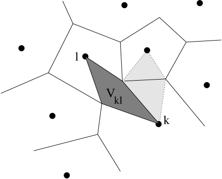
FIG. 4.: Pairwise Voronoi-cell interactions. Dark gray: The volume $V_{kl}$ associated with the interaction between a single DP-pair. The light gray region shows the volume of the neighboring interaction.

By making the identifications $\zeta=(2/d)\eta$, ${\bf n}\rightarrow{\bf e}_{kl}$ $\tilde{{\bf F}}_{kl}=l_{kl}{\bf s}\cdot{\bf e}_{kl}$, $\Delta V_{n}\rightarrow V_{kl}$, (shown in Fig. 4), and $T=\Theta_{kl}$ we may immediately write down

$$\langle\tilde{{\bf F}}_{kl}(t)\tilde{{\bf F}}_{nm}(0)\rangle = 2\frac{k_{B}\Theta_{kl}l_{kl}^{2}}{V_{kl}}\eta(1+{\bf e}_{kl}{\bf e}_{nm})\delta(t)$$ (118)

$$( \delta_{kn}\delta_{lm}+\delta_{km}\delta_{ln})$$ (119)

where again the last sum of $\delta$-factors ensures that $kl$ and $nm$ denote the same DP pair. Observing from Fig. 4 that $V_{kl}=l_{kl}r_{kl}$, it now follows directly from Eq. (119) that

$$\langle\tilde{{\bf F}}_{kl}(t)\cdot{\bf e}_{kl}\tilde{{\bf F}}_{nm}(0)\cdot{\bf e}_{nm}\rangle = 2\langle\tilde{{\bf F}}_{kl}(t)\cdot{\bf i}_{kl}\tilde{{\bf F}}_{nm}(0)\cdot{\bf i}_{nm}\rangle$$ (120)

$$= 4k_{B}\Theta_{kl}\frac{l_{kl}}{r_{kl}}\eta\delta(t)$$ (121)

$$( \delta_{kn}\delta_{lm}+\delta_{km}\delta_{ln})$$ (122)

which is nothing but the momentum part of Eq. (112). That the fluctuating heat flux $\tilde{q}$ produces the form of fluctuation-dissipation relations given in Eq. (112) follows from a similar analysis. Thus the approximation of fixed DP volume $V_{k}$ produces the same result as the approximation of fixed number of MD particles $N_{k}$. This is due to the fact that both approximations are based on the assumption that the DP’s are only considered within a time interval which is longer than the correlation time of the fluctuations but shorter than the time needed for the DP’s to move significantly.

The result given in Eq. (122) was derived from the somewhat arbitrary choice of discretizaton volume $V_{kl}$; this is the volume which corresponds to the segment $l_{kl}$ over which all forces have been taken as constant. It is thus the smallest discretization volume we may consistently choose. It is reassuring that Eq. (122) also follows from different choices of $\Delta V_{n}$. For example, one may readily check that Eq. (122) is obtained if we split $V_{kl}$ in two along $r_{kl}$ and consider $\tilde{{\bf F}}_{kl}$ to be the sum of two independent forces acting on the two parts of $l_{kl}$.

We are now in a position to quantify the average component $\langle\dot{\tilde{E}}_{k}\rangle\equiv\sum_{l\neq k}\langle\tilde{{\bf F}}_{kl}\cdot{\bf U}_{kl}/2\rangle$ of the fluctuations in the internal energy given in Eq. (83). Writing the velocity in response to $\tilde{{\bf F}}_{kl}$ as $\tilde{{\bf U}}_{k}=\sum_{l\neq k}\int_{-\infty}^{t}\text{d}t^{\prime}\tilde{F}_{kl}(t^{\prime})/M_{k}$, we get that $\langle\dot{\tilde{E}}_{k}\rangle=\sum\int_{-\infty}^{t}\text{d}t^{\prime}\langle\tilde{F}_{kl}(t^{\prime})\tilde{F}_{kl}(t)\rangle$ which by Eqs. (112) and (95) becomes $\langle\dot{\tilde{E}}_{k}\rangle=(1/M_{k})\sum 3l_{kl}\eta k_{B}\Theta_{kl}/r_{kl}$. This result is the same as one would have obtained applying the rules of Itô calculus to $\tilde{{\bf U}}_{k}^{2}/(2M_{k})$. It yields the modified, though equivalent, energy equation

$$\dot{E}_{k}=-\sum_{l}l_{lk}\lambda\frac{T_{kl}}{r_{kl}}$$ (123)

$$- \sum_{l}l_{lk}\left(\frac{p_{k}+p_{l}}{2}{\bf e}_{kl}-\frac{\eta}{r_{kl}}({\bf U}_{kl}+({\bf U}_{kl}\cdot{\bf e}_{kl}){\bf e}_{kl})\right)\cdot\frac{{\bf U}_{kl}}{2}$$ (124)

$$- \sum_{l}\tilde{{\bf F}^{\prime}}_{kl}\cdot\frac{{\bf U}_{kl}}{2}-3\frac{l_{kl}}{r_{kl}}\eta k_{B}\Theta_{kl}+\tilde{q}_{kl}\;.$$ (125)

where we have written $\tilde{{\bf F}^{\prime}}_{kl}$ with a prime to denote that it is uncorrelated with ${\bf U}_{kl}$. In a numerical implementation this implies that $\tilde{{\bf F}^{\prime}}_{kl}$ must be generated from a different random variable than $\tilde{{\bf F}}_{kl}$, which was used to update ${\bf U}_{kl}$.

The fluctuation-dissipation relations Eqs. (112) complete our theoretical description of dissipative particle dynamics, which has been derived by a coarse-graining of molecular dynamics. All the parameters and properties of this new version of DPD are related directly to the underlying molecular dynamics, and properties such as the viscosity which are emergent from it.

V Simulations

While the present paper primarily deals with theoretical developments we have carried out simulations to test the equilibrium behavior of the model in the case of the isothermal model. This is a crucial test as the derivation of the fluctuating forces relies on the most significant approximations. The simulations are carried out using a periodic Voronoi tesselation described in detail elsewhere [29].

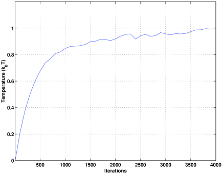
FIG. 5.: The DPD temperature (energy units) averaged over 5000 dissipative particles as a function of time (iteration number in the integration scheme), showing good convergence to the underlying molecular dynamics temperature which was set at one. This simulation provides strong support for the approximations used to derive the fluctuation-dissipation relations in our DPD model from molecular dynamics.

Figure 5 shows the relaxation process towards equilibrium of an initially motionless system. The DP temperature is measured as $\langle{\bf P}_{k}^{2}/(2M_{k})\rangle$ for a system of DPs with internal energy equal to unity. The simulations were run for 4000 iterations of 5000 dissipative particles and a timestep $\text{d}t=0.0005$ using an initial molecular density $\rho=5$ for each DP. The molecular mass was taken to be $m=1$, the viscosity was set at $\eta=1$, the expected mean free path is 0.79, and the Reynolds number (See Sec. VI B) is Re=2.23. It is seen that the convergence of the DP system towards the MD temperature is good, a result that provides strong support for the fluctuation-dissipation relations of Eq. (112).

VI Possible applications

A Multiscale phenomena

For most practical applications involving complex fluids, additional interactions and boundary conditions need to be specified. These too must be deduced from the microscopic dynamics, just as we have done for the interparticle forces. This may be achieved by considering a particulate description of the boundary itself and including molecular interactions between the fluid MD particles and other objects, such as particles or walls. Appropriate modifications can then be made on the basis of the momentum-flux tensor of Eq. (32), which is generally valid.

Consider for example the case of a colloidal suspension, which is shown in Fig. 6. Beginning with the hydrodynamic momentum-flux tensor Eq. (32) and Eq. (71), it is evident that we also need to define an interaction region where the DP–colloid forces act: the DP–colloid interaction may be obtained in the same form as the DP–DP interaction of Eq. (71) by making the replacement $l_{kl}\rightarrow L_{kI}$, where $L_{kI}$ is the length (or area in 3D) of the arc segment where the dissipative particle meets the colloid (see Fig. 6) and the velocity gradient $r_{kl}^{-1}(({\bf U}_{kl}\cdot{\bf e}_{kl}){\bf e}_{kl}+{\bf U}_{kl})$ is that between the dissipative particle and the colloid surface. The latter may be computed using ${\bf U}_{k}$ and the velocity of the colloid surface together with a no-slip boundary condition on this surface. In Eq. (112) the replacement $l_{kl}\rightarrow L_{KI}$ must also be made.

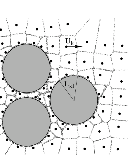
FIG. 6.: Multiscale modeling of colloidal fluids. As usual, the dissipative particles are defined as cells in the Voronoi lattice. Note that there are four relevant length scales in this problem: the scale of the large, gray colloid particles, the two distinct scales of the dissipative particles in between and away from the colloids and finally the molecular scale of the MD particles. These mediate the mesoscopic interactions and are shown as dots on the boundaries between dissipative and colloidal particles.

Although previous DPD simulations of colloidal fluids have proved rather successful [10] at low to intermediate solids volume fractions, they break down for dense systems whose solids volume fraction exceeds a value of about 40% because the existing method is unable to handle multiple lengthscale phenomena. However, our new version of the algorithm provides the freedom to define dissipative particle sizes according to the local resolution requirements as illustrated in Fig. 6. In order to increase the spatial resolution where colloidal particles are within close proximity it is necessary and perfectly admissible to introduce a higher density of dissipative particles there; this ensures that fluid lubrication and hydrodynamic effects are properly maintained. After these dissipative particles have moved it may be necessary to re-tile the DP system; this is easily achieved by distributing the mass and momentum of the old dissipative particles on the new ones according to their area (or volume in 3D). Considerations of space prevent us from discussing this problem further in the present paper, but we plan to report in detail on such dense colloidal particle simulations using our method in future publications. We note in passing that a wide variety of other complex systems exist where modeling and simulation are challenged by the presence of several simultaneous length scales, for example in polymeric and amphiphilic fluids, particularly in confined geometries such as porous media [30].

B The low viscosity limit and high Reynolds numbers

In the kinetic theory derived by Marsh, Backx and Ernst [15] the viscosity is explicitly shown to have a kinetic contribution $\eta_{K}=\rho D/2$ where $D$ is the DP self diffusion coefficient and $\rho$ the mass density. The kinetic contribution to the viscosity was measured by Masters and Warren [31] within the context of an improved theory. How then can the viscosity $\eta$ used in our model be decreased to zero while kinetic theory puts the lower limit $\eta_{K}$ to it?

To answer this question we must define a physical way of decreasing the MD viscosity while keeping other quantities fixed, or, alternatively rescale the system in a way that has the equivalent effect. The latter method is preferable as it allows the underlying microscopic system to remain fixed. In order to do this we non-dimensionalize the DP momentum equation Eq. (71).

For this purpose we introduce the characteristic equilibrium velocity, $U_{0}=\sqrt{k_{B}T/M}$, the characteristic distance $r_{0}$ as the typical DP size. Then the characteristic time $t^{\prime}=r_{0}/U_{0}$ follows.

Neglecting gravity for the time being Eq. (71) takes the form

$$\frac{\text{d}{\bf P}_{k}^{\prime}}{\text{d}t^{\prime}}=-\sum_{l}l^{\prime}_{kl}\left(\frac{p^{\prime}_{kl}}{2}{\bf e}_{kl}+\frac{1}{\text{Re}}\left({\bf U}^{\prime}_{kl}+({\bf U}^{\prime}_{kl}\cdot{\bf e}_{kl}){\bf e}_{kl}\right)\right)$$ (126)

$$+ \sum_{l}\frac{l^{\prime}_{kl}L^{\prime}_{kl}}{2r^{\prime}_{kl}}\frac{\rho^{\prime}_{k}+\rho^{\prime}_{l}}{2}{\bf i}_{kl}\cdot{\bf U}^{\prime}_{kl}\frac{{\bf U}^{\prime}_{k}+{\bf U}^{\prime}_{l}}{2}+\sum_{l}\tilde{{\bf F}}^{\prime}_{kl}\;,$$ (127)

where ${\bf P}_{k}^{\prime}={\bf P}_{k}/(MU_{0})$, $p^{\prime}_{kl}=p_{kl}r_{0}^{2}/(MU_{0}^{2})$, $M=\rho r_{0}^{2}$ in 2d, the Reynolds number $\text{Re}=U_{0}r_{0}\rho/\eta$ and $\tilde{{\bf F}}^{\prime}_{kl}=(r_{0}/MU_{0}^{2})\tilde{{\bf F}}_{kl}$ where $\tilde{{\bf F}}_{kl}$ is given by Eqs. (90) and (112). A small calculations then shows that if $\tilde{{\bf F}}^{\prime}_{kl}$ is related to $\omega_{kl}^{\prime}$ and $t^{\prime}$ like $\tilde{{\bf F}}_{kl}$ related to $\omega_{kl}$ and $t$, then

$$\omega_{kl}^{{}^{\prime}2}\approx\frac{1}{\text{Re}}\frac{k_{B}T}{MU_{0}^{2}}\approx\frac{1}{\text{Re}}$$ (128)

where we have neglected dimensionless geometric prefactors like $l_{kl}/r_{kl}$ and used the fact that the ratio of the thermal to kinetic energy by definition of $U_{0}$ is one.

The above results imply that when the DPD system is measured in non-dimensionalized units everything is determined by the value of the mesoscopic Reynolds number Re. There is thus no observable difference in this system between increasing $r_{0}$ and decreasing $\eta$.

Returning to dimensional units again the DP diffusivity may be obtained from the Stokes-Einstein relation [32] as

$$D=\frac{k_{B}T}{ar_{0}\eta}$$ (129)

where $a$ is some geometric factor ($a=6\pi$ for a sphere) and all quantities on the right hand side except $r_{0}$ refer directly to the underlying MD. As we are keeping the MD system fixed and increasing Re by increasing $r_{0}$, it is seen that $D$ and hence $\eta_{K}$ vanish in the process.

We note in passing that if $D$ is written in terms of the mean free path $\lambda$: $D=\lambda\sqrt{k_{B}T/(\rho r_{0}^{2})}$ and this result is compared with Eq. (129) we get $\lambda^{\prime}=\lambda/r_{0}\sim 1/r_{0}$ in 2d, i.e. the mean free path, measured in units of the particle size decreases as the inverse particle size. This is consistent with the decay of $\eta_{K}$. The above argument shows that decreasing $\eta$ is equivalent to keeping the microscopic MD system fixed while increasing the DP size, in which case the mean free path effects on viscosity is decreased to zero as the DP size is increased to infinity. It is in this limit that high Re values may be achieved.

Note that in this limit the thermal forces $\tilde{{\bf F}}_{kl}\sim\text{Re}^{-1/2}$ will vanish, and that we are effectively left with a macroscopic, fluctuationless description. This is no problem when using the present Voronoi construction. However, the effectively spherical particles of conventional DPD will freeze into a colloidal crystal, i.e. into a lattice configuration [8,9] in this limit. Also while conventional DPD has usually required calibration simulations to determine the viscosity, due to discrepancies between theory and measurements, the viscosity in this new form of DPD is simply an input parameter. However, there may still be discrepancies due to the approximations made in going from MD to DPD. These approximations include the linearization of the inter-DP velocity fields, the Markovian assumption in the force correlations and the neglect of a DP angular momentum variable.

None of the conclusions from the above arguments would change if we had worked in three dimensions in stead of two.

VII Conclusions

We have introduced a systematic procedure for deriving the mesoscopic modeling and simulation method known as dissipative particle dynamics from the underlying description in terms of molecular dynamics.

FIG. 7.: Outline of the derivation of dissipative particle dynamics from molecular dynamics as presented in the present paper. The MD viscosity is denoted by $\eta$ and $\omega$ is the amplitude of the fluctuating force $\tilde{\bf F}$ as defined in Eq. (90)

Figure 7 illustrates the structure of the theoretical development of DPD equations from MD as presented in this paper. The initial coarse graining leads to equations of essentially the same structure as the final DPD equations. However, they are still invariant under time- reversal. The label DPD1 refers to Eqs. (58), (62) and (75), whereas the DPD2 equations have been supplemented with specific constitutive relations both for the non-equilibrium fluxes (momentum and heat) and an equilibrium description of the thermodynamics. These equations are Eqs. (71) and (83) along with Eqs. (112). The development we have made which is shown in Fig. 7 does not claim to derive the irreversible DPD equations from the reversible ones of molecular dynamics in a rigorous manner, although it does illustrate where the transition takes place with the introduction of molecular averages. The kinetic equations of this new DPD satisfy an $H$-theorem, guaranteeing an irreversible approach to the equilibrium state. Note that in passing to the time-asymmetric description by the introduction of the averaged description of Eq. (66), a time asymmetric non-equilibrium ensemble is required [23].

This is the first time that any of the various existing mesoscale methods have been put on a firm ‘bottom up’ theoretical foundation, a development which brings with it numerous new insights as well as practical advantages. One of the main virtues of this procedure is the capability it provides to choose one or more coarse-graining lengthscales to suit the particular modeling problem at hand. The relative scale between molecular dynamics and the chosen dissipative particle dynamics, which may be defined as the ratio of their number densities $\rho_{\text{DPD}}/\rho_{\text{MD}}$, is a free parameter within the theory. Indeed, this rescaling may be viewed as a renormalisation group procedure under which the fluid viscosity remains constant: since the conservation laws hold exactly at every level of coarse graining, the result of doing two rescalings, say from MD to DPD$\alpha$ and from DPD$\alpha$ to DPD$\beta$, is the same as doing just one with a larger ratio, i.e. $\rho_{\text{DPD}\beta}/\rho_{\text{MD}}=(\rho_{\text{DPD}\beta}/\rho_{\text{DPD}\alpha})(\rho_{\text{DPD}\alpha}/\rho_{\text{MD}})$.

The present coarse graining scheme is not limited to hydrodynamics. It could in principle be used to rescale the local description of any quantity of interest. However, only for locally conserved quantities will the DP particle interactions take the form of surface terms as here, and so it is unlikely that the scheme will produce a useful description of non-conserved quantities.

In this context, we note that the bottom-up approach to fluid mechanics presented here may throw new light on aspects of the problem of homogeneous and inhomogeneous turbulence. Top-down multiscale methods and, to a more limited extent, ideas taken from renormalisation group theory have been applied quite widely in recent years to provide insight into the nature of turbulence [33, 34]; one might expect an alternative perspective to emerge from a fluid dynamical theory originating at the microscopic level, in which the central relationship between conservative and dissipative processes is specified in a more fundamental manner. From a practical point of view it is noted that, since the DPD viscosity is the same as the viscosity emergent from the underlying MD level, it may be treated as a free parameter in the DPD model, and thus high Reynolds numbers may be reached. In the $\eta\rightarrow 0$ limit the model thus represents a potential tool for hydrodynamic simulations of turbulence. However, we have not investigated the potential numerical complications of this limit.

The dissipative particle dynamics which we have derived is formally similar to the conventional version, incorporating as it does conservative, dissipative and fluctuating forces. The interactions are pairwise, and conserve mass and momentum as well as energy. However, now all these forces have been derived from the underlying molecular dynamics. The conservative and dissipative forces arise directly from the hydrodynamic description of the molecular dynamics and the properties of the fluctuating forces are determined via a fluctuation–dissipation relation.

The simple hydrodynamic description of the molecules chosen here is not a necessary requirement. Other choices for the average of the general momentum and energy flux tensors Eqs. (46) and (32) may be made and we hope these will be explored in future work. More significant is the fact that our analysis permits the introduction of specific physicochemical interactions at the mesoscopic level, together with a well-defined scale for this mesoscopic description.

While the Gaussian basis we used for the sampling functions is an arbitrary albeit convenient choice, the Voronoi geometry itself emerged naturally from the requirement that all the MD particles be fully accounted for. Well defined procedures already exist in the literature for the computation of Voronoi tesselations [35] and so algorithms based on our model are not computationally difficult to implement. Nevertheless, it should be appreciated that the Voronoi construction represents a significant computational overhead. This overhead is of order $N\log N$, a factor $\log N$ larger than the most efficient multipole methods in principle available for handling the particle interactions in molecular dynamics. However, the prefactors are likely to be much larger in the particle interaction case.

Finally we note the formal similarity of the present particulate description to existing continuum fluid dynamics methods incorporating adaptive meshes, which start out from a top-down or macroscopic description. These top-down approaches include in particular smoothed particle hydrodynamics [19] and finite-element simulations. In these descriptions too the computational method is based on tracing the motion of elements of the fluid on the basis of the forces acting between them [36]. However, while such top-down computational strategies depend on a macroscopic and purely phenomenological fluid description, the present approach rests on a molecular basis.

- [1] L. D. Landau and E. M. Lifshitz, Fluid Mechanics (Pergamon Press, New York, 1959).
- [2] L. Boltzmann., Vorlesungen über Gastheorie (Leipzig, 1872).
- [3] J. Koplik and J. R. Banavar, Ann. Rev. Fluid Mech. 27, 257 (1995).
- [4] U. Frisch, B. Hasslacher, and Y. Pomeau, Phys. Rev. Lett. 56, 1505 (1986).
- [5] G. McNamara and G. Zanetti, Phys. Rev. Lett. 61, 2332 (1988).
- [6] X. W. Chan and H. Chen, Phys. Rev E 49, 2941 (1993).
- [7] M. R. Swift, W. R. Osborne, and J. Yeomans, Phys. Rev. Lett. 75, 830 (1995).
- [8] P. J. Hoogerbrugge and J. M. V. A. Koelman, Europhys. Lett. 19, 155 (1992).
- [9] P. Español and P. Warren, Europhys. Lett. 30, 191 (1995).
- [10] E. S. Boek, P. V. Coveney, H. N. W. Lekkerkerker, and P. van der Schoot, Phys. Rev. E 54, 5143 (1997).
- [11] A. G. Schlijper, P. J. Hoogerbrugge, and C. W. Manke, J. Rheol. 39, 567 (1995).
- [12] P. V. Coveney and K. E. Novik, Phys. Rev. E 54, 5143 (1996).
- [13] R. D. Groot and P. B. Warren., J. Chem. Phys. 107, 4423 (1997).
- [14] P. Español, Phys. Rev. E 52, 1734 (1995).
- [15] C. A. Marsh, G. Backx, and M. Ernst, Phys. Rev. E 56, 1676 (1997).
- [16] J. B. Avalos and A. D. Mackie, Europhys. Lett. 40, 141 (1997).
- [17] P. Español, Europhys. Lett 40, 631 (1997).
- [18] P. Español, Phys. Rev. E 57, 2930 (1998).
- [19] J. J. Monaghan, Ann. Rev. Astron. Astophys. 30, 543 (1992).
- [20] P. Español, M. Serrano, and I. Zuñiga, Int. J. Mod. Phys. C 8, 899 (1997).
- [21] E. G. Flekkøy and P. V. Coveney, Phys. Rev. Lett. 83, 1775 (1999).
- [22] P. V. Coveney and O. Penrose, J. Phys A: Math. Gen. 25, 4947 (1992).
- [23] O. Penrose and P. V. Coveney, Proc. R. Soc. 447, 631 (1994).
- [24] P. V. Coveney and R. Highfield, The Arrow of Time (W. H.Allen, London, 1990).
- [25] C. A. Marsh and P. V. Coveney, J. Phys. A: Math. Gen. 31, 6561 (1998).
- [26] F. Reif, Fundamentals of statistical and thermal physics (Mc Graw-Hill, Singapore, 1965).
- [27] L. D. Landau and E. M. Lifshitz, Statistical Physics (Pergamon Press, New York, 1959).
- [28] C. W. Gardiner, Handbook of stochastic methods (Springer Verlag, Berlin Heidelberg, 1985).
- [29] G. D. Fabritiis, P. V. Coveney, and E. G. Flekkøy, in Proc. 5th European SGI/Cray MPP Workshop, Bologna, Italy 1999.
- [30] P. V. Coveney, J. B. Maillet, J. L. Wilson, P. W. Fowler, O. Al-Mushadani and B. M. Boghosian, Int. J. Mod. Phys. C 9, 1479 (1998).
- [31] A. J. Masters and P. B. Warren, preprint cond-mat/9903293 (http://xxx.lanl.gov/) (unpublished).
- [32] A. Einstein, Ann. Phys. 17, 549 (1905).
- [33] U. Frisch, Turbulence (Cambridge University Press, Cambridge, 1995).
- [34] A. Bensoussan, J. L. Lions, and G. Papanicolaou, Asymptotic Analysis for Periodic Structures (North-Holland, Amsterdam, 1978).
- [35] D. E. K. L. J. Guibas and M. Sharir, Algorithmica 7, 381 (1992).
- [36] B. M. Boghosian, Encyclopedia of Applied Physics 23, 151 (1998).