Coexistent State of Charge Density Wave and Spin Density Wave in One-Dimensional Quarter Filled Band Systems under Magnetic Fields

1 Introduction

It is found that the system with the one-dimensional quarter filled band becomes the coexistent state of the charge density wave (CDW) and spin density wave (SDW) due to the interplay between the on-site Coulomb interaction ($U$) and the inter-site Coulomb interaction ($V$) by recent theoretical works.${}^{\hbox{\immediate{\bf{?}},\penalty 1000\hskip 0.91003pt plus 0.70004pt minus 0.70004pt{\bf{?}},\penalty 1000\hskip 0.91003pt plus 0.70004pt minus 0.70004pt{\bf{?}},\penalty 1000\hskip 0.91003pt plus 0.70004pt minus 0.70004pt{\bf{?}})}}$ The inter-site Coulomb interaction plays important role of the charge ordering, and the ground state is the coexistent state of $2k_{\rm F}$-SDW and $4k_{\rm F}$-CDW,${}^{\hbox{\immediate{?})}}$ where $k_{\rm F}$ is Fermi wave vector, $k_{\rm F}=\pi/4a$ and $a$ is the lattice constant. Furthermore, when the next nearest neighbor and the dimerization of the energy band are considered, it has been indicated that $2k_{\rm F}$-SDW and $2k_{\rm F}$-CDW coexist.${}^{\hbox{\immediate{?},\penalty 1000\hskip 0.91003pt plus 0.70004pt minus 0.70004pt{?})}}$

Quasi-one dimensional organic conductors such as (TMTSF)₂$X$ and (TMTTF)₂$X$ ($X$=ClO₄, PF₆, AsF₆, ReO₄, Br, SCN, etc.) are known as the one-dimensional quarter filled band and exhibit many kinds of ground state, for example, spin-Peierls, SDW, superconductivity.${}^{\hbox{\immediate{\bf{?}},\penalty 1000\hskip 0.91003pt plus 0.70004pt minus 0.70004pt{\bf{?}})}}$ In (TMTSF)₂PF₆, the incommensurate SDW is occurred at $T=12$ K, where the wave vector is (0.5, 0.24,-0.06) by NMR measurement.${}^{\hbox{\immediate{\bf{?}},\penalty 1000\hskip 0.91003pt plus 0.70004pt minus 0.70004pt{\bf{?}})}}$ Recently, from the X-ray measurement, Pouget and Ravy argue the coexistence of $2k_{\rm F}$-SDW and $2k_{\rm F}$-CDW,${}^{\hbox{\immediate{\bf{?}})}}$ which has been theoretically explained by Kobayashi et al.${}^{\hbox{\immediate{?},\penalty 1000\hskip 0.91003pt plus 0.70004pt minus 0.70004pt{?})}}$ mentioned above and Mazumdar et al..${}^{\hbox{\immediate{?})}}$

On the other hand, in (TMTTF)₂$X$, (X=Br and SCN), it is known that the ground state is the antiferromagnetic phase understood as Mott-Hubbard inslator phase due to the dimerization and the quarter filling. It is clear that the wave vector of the SDW is commesurate, (0.5, 0.25,0) from the measurements of ¹³C-NMR${}^{\hbox{\immediate{\bf{?}})}}$ and ¹H-NMR.${}^{\hbox{\immediate{\bf{?}})}}$ From the angle depenence of satelite peak positions of ¹H-NMR,${}^{\hbox{\immediate{?},\penalty 1000\hskip 0.91003pt plus 0.70004pt minus 0.70004pt{\bf{?}})}}$ the alignment of the spin moment along the conductive axis (a-axis) becomes ($\uparrow,0,\downarrow,0$), which corresponds to the recent calculational results.${}^{\hbox{\immediate{?},\penalty 1000\hskip 0.91003pt plus 0.70004pt minus 0.70004pt{\bf{?}})}}$ In (TMTTF)₂Br, $4k_{\rm F}$-CDW accompanied by $2k_{\rm F}$-SDW is found in X-ray measurments.${}^{\hbox{\immediate{?})}}$ This can be explained by Seo and Fukuyama${}^{\hbox{\immediate{?})}}$ by using the extended Hubbard model.

When the pressure is applied, the commensurate antiferromagnetic phase in (TMTTF)₂Br at ambient pressure changes to the incommensurate SDW phase such as (TMTSF)₂$X$.${}^{\hbox{\immediate{\bf{?}})}}$ It is originated to the increasing of the hopping transfer integral, $t$. In the case of small $t$, as the exchange interaction is strongly influenced, the state becomes Mott antiferromagnetic state. When $t$ becomes large, the system becomes the SDW phase due to the Peierls instability of the Fermi surface. The difference between (TMTTF)₂$X$ and (TMTSF)₂$X$ is whether the charge or spin ordering is localized or not. This difference is attributed that $U/t$ in (TMTTF)₂$X$ is larger than that in (TMTSF)₂$X$. It is indicated that $U/t\simeq 5.0$ (3.0) in (TMTTF)₂$X$ ((TMTSF)₂$X$) since $t$ in (TMTTF)₂$X$ ((TMTSF)₂$X$) are about 0.2 (0.3) eV by the extended Huckel band calculations. ${}^{\hbox{\immediate{\bf{?}},\penalty 1000\hskip 0.91003pt plus 0.70004pt minus 0.70004pt{\bf{?}},\penalty 1000\hskip 0.91003pt plus 0.70004pt minus 0.70004pt{\bf{?}},\penalty 1000\hskip 0.91003pt plus 0.70004pt minus 0.70004pt{\bf{?}})}}$ We consider the system in (TMTTF)₂$X$ ((TMTSF)₂$X$) as strongly (non-strongly) correlated.

In the one-dimensional system, when the magnetic field ($H$) is applied to $c$-axis, the amplitudes of the charge density or the spin moment along the $c$-axis in the CDW or SDW state by coupling of electrons with same spins are suppressed due to Pauli paramagnetic limit field ($H_{p}$),${}^{\hbox{\immediate{\bf{?}},\penalty 1000\hskip 0.91003pt plus 0.70004pt minus 0.70004pt{\bf{?}},\penalty 1000\hskip 0.91003pt plus 0.70004pt minus 0.70004pt{\bf{?}})}}$ where $H_{p}\simeq\Delta(0)/\sqrt{2}\mu_{\rm B}$, $\Delta(0)$ is the amplitude of the energy gap at $H=0$ and $\mu_{\rm B}=e\hbar/2m_{0}c$ is the Bohr magneton. The energy band is splitted by Zeeman effect, so that the original wave vector at $H=0$ becomes the not good nesting vector. In the case of the magnetic field applied along the $a$- or $b$-axis, the CDW and SDW are not broken, because the nesting vector is unchanged by Zeeman effect. In other words, the CDW and SDW are not influenced when the magnetic field is applied perpendicular to the easy axis. This picture is for the weak coupling system.

In the strong coupling system, the $H$-dependence of the antiferromagnetic state by one-dimensional Ising model has been studied in the mean field approximation.${}^{\hbox{\immediate{\bf{?}})}}$ The amplitude of the spin moment along the $c$-axis of the antiferromagnetic state under magnetic fields applied along the $a$-axis is easily obtained, which obey

$$S_{z}(H,j)/S_{z}(0,j)=\sqrt{1-(H/H_{x}^{0})^{2}},$$ (1)

where $S_{z}(H,j)$ is the amplitude of the spin moment along the $c$-axis at $j$ site at $H=0$ and $H_{x}^{0}$ is the critical field at which the ordering of the antiferromagnetic state disappear.${}^{\hbox{\immediate{?})}}$ Since the spin of electrons are tilted to $a$-axis by the magnetic field, $S_{z}$ is smaller upon increasing $H_{x}$, finally, $S_{z}$ becomes zero.

In the case of magnetic fields applied to the $c$-axis, the antiferromagnetic state along the $c$-axis is kept, because if the spin is tilted to $a$-$b$ plane, this tilted state is not unstable in weak fields. However, the paramagnetic state becomes more stable at higher critical field, $H_{z}^{0}$, where $H_{z}^{0}=H_{x}^{0}$, ${}^{\hbox{\immediate{?})}}$

We try to analyze the coexistent state in the two cases when the electron correlation is strong or not, since the coexistent phase of CDW and SDW under magnetic fields dose not have been studied although the state of CDW or SDW under magnetic fields has been studied. When $U/t$ and $V/t$ are large ($\sim 5.0$), we consider that the system is strongly correlated, because the charge and spin are localized as shown in Figs. 1 and 2. On the other hand, in small $U/t$ and $V/t$ ($\sim 1.5$), the correlation between electrons is not strong, where there are small amplitudes of charge density and spin moment as shown in Fig. 7, 8 and 9. We calculate to compare the strong coupling system with the non-strong coupling system by using of two sets of the values of $U/t$ and $V/t$.

In this paper, we calculate the self-consistent solutions at $T=0$ for the one-dimensional band model under the magnetic field perpendicular to (or parallel to) the a-axis based on the mean field approximation. We use the one-dimensional quarter filled extended Hubbard model, where the effect of the dimerization do not be considered to be simplified problems.

2 Formulation

We treat the one-dimensional extended Hubbard model,

$$\hat{\cal H} = \hat{\cal K}+\hat{\cal U}+\hat{\cal V},$$ (2)

$$\hat{\cal K} = t\sum_{i,\sigma}(C^{\dagger}_{i,\sigma}C_{i+1,\sigma}+h.c.)-\frac{\mu_{\rm B}gH_{j}}{2}\sum_{i,\sigma}n_{i,\sigma},$$ (3)

$$\hat{\cal U} = U\sum_{i}n_{i,\uparrow}n_{i,\downarrow},$$ (4)

$$\hat{\cal V} = V\sum_{i,\sigma,\sigma^{\prime}}n_{i,\sigma}n_{i+1,\sigma^{\prime}},$$ (5)

where $C^{\dagger}_{i,\sigma}$ is the creation operator of $\sigma$ spin electron at $i$ site, $n_{i,\sigma}$ is the number operator, $g=2$, $i=1,\cdots,N_{\rm S}$, $N_{\rm S}$ is the number of the total sites and $\sigma=\uparrow$ and $\downarrow$. When the magnetic field is applied to (x or z)-axis ($H_{x}$ or $H_{z}$), $H_{j}=H\hat{\sigma}_{j}$ ($j=x$ and $z$), where $H$ is the strength of the magnetic field and $\hat{\sigma}_{j}$ is Pauli spin matrix. In this model, the filling of electrons is 1/4.

The interaction term, $\hat{\cal U}$ and $\hat{\cal V}$ are treated in mean field approximation as

$$\hat{\cal U}_{\rm M} = \sum_{k_{x}}\sum_{Q}\{\rho_{\uparrow}(Q)C^{\dagger}(k_{x},\downarrow)C(k_{x}-Q,\downarrow)$$ (6)

$$+ \rho^{*}_{\downarrow}(Q)C^{\dagger}(k_{x}-Q,\uparrow)C(k_{x},\uparrow)\}$$

$$- \frac{1}{I}\sum_{Q}\rho_{\uparrow}(Q)\rho^{*}_{\downarrow}(Q),$$

$$\hat{\cal V}_{\rm M} = (\frac{V}{U})\sum_{k_{x},\sigma,\sigma^{\prime}}\sum_{Q}e^{-iQa}\{\rho_{\sigma}(Q)C^{\dagger}(k_{x},\sigma^{\prime})C(k_{x}-Q,\sigma^{\prime})$$ (7)

$$+ \rho_{\sigma^{\prime}}^{*}(Q)C^{\dagger}(k_{x},\sigma)C(k_{x}-Q,\sigma)\}$$

$$- \frac{V}{IU}\sum_{Q,\sigma,\sigma^{\prime}}e^{-iQa}\rho_{\sigma}(Q)\rho_{\sigma^{\prime}}^{*}(Q),$$

where $I=U/N_{\rm S}$. The self-consistent equation for the order parameter $\rho_{\sigma}(Q)$ is given by

$$\rho_{\sigma}(Q) = I\sum_{k_{x}}<C^{\dagger}(k_{x},\sigma)C(k_{x}-Q,\sigma)>.$$ (8)

We use the mean field, $\rho_{\sigma}(Q)$, by the coupling between electrons with same spins. In order to simplify, we do not consider the case of the mean field, $\bar{\rho_{\sigma}}(Q)=I\sum_{k_{x}}<C^{\dagger}(k_{x},\sigma)C(k_{x}-Q,\bar{\sigma})>$, by the coupling of electrons with opposite spin.

We limit the sum of the wave vector as $Q=q,2q,3q$ and $4q$ ($q=2k_{\rm F}$), because the wave vectors of $2k_{\rm F}=\pi/2a$ and its higher harmonics should be considered due to the nesting of the Fermi surface in the one-dimensional quarter filled band. We can obtain the self-consistent solutions from eq. (8) by using eigenvectors obtained by diagonalizing $\hat{\cal K}+\hat{\cal U}_{\rm M}+\hat{\cal V}_{\rm M}$, which becomes $8\times 8$ matrix. The electron density at $j$ site, $n(j)$, and the spin moment at $j$ site, $S_{z}(j)$, are given by

$$n(j) = \frac{1}{U}\sum_{Q,\sigma}\rho_{\sigma}(Q)e^{iQja},$$ (9)

$$S_{z}(j) = \frac{1}{2U}\sum_{Q}(\rho_{\uparrow}(Q)-\rho_{\downarrow}(Q))e^{iQja}.$$ (10)

The notation in this paper follows Seo and Fukuyama.${}^{\hbox{\immediate{?})}}$ We can calculate the total energy, $E$,

$$E=\sum_{i=1,\sigma}\epsilon_{i,\sigma},$$ (11)

where the sum is limited to electron filling and $\epsilon_{i,\sigma}$ is an eigenvalue. From the ordered state energy ($E_{\rm OS}$) and the normal state energy ($E_{\rm N}$), the energy gain ($E_{\rm g}$) can be obtained by $E_{\rm g}=E_{\rm OS}-E_{\rm N}$.

The Pauli spin susceptibility, $\chi$, is $\mu_{\rm B}^{2}N(0)$ ($N(0)$ is the density of state on the Fermi energy and $N(0)=N_{\rm S}/(4\pi t\sin ak_{\rm F})$),${}^{\hbox{\immediate{?},\penalty 1000\hskip 0.91003pt plus 0.70004pt minus 0.70004pt{?},\penalty 1000\hskip 0.91003pt plus 0.70004pt minus 0.70004pt{?})}}$ and the energy gain from the normal state is given by $-\chi H^{2}$. When $E_{\rm g}=-\chi H_{p}^{2}$, the Pauli limit field, $h_{p}$, is given by

$$h_{p}=2\sqrt{\frac{-\pi E_{\rm g}}{\sqrt{2}N_{\rm S}}},$$ (12)

where $h_{p}=\mu_{\rm B}gH_{p}/2t$.

Fig.  1: 2S_z as a function of $v$ at $H=0$

Fig.  2: $\delta$ as a function of $v$ at $H=0$

3 Results and Discussions

3.1 Strong coupling

First, we show the result at $H=0$ at $U/t=5.0$, whose large value means the strongly correlated system. Figs. 1 and 2 are $S_{z}$ and $\delta$ as a function of $V/t$ at $U/t=5.0$. At $0\leq V\leq 0.392$, the antiferromagnetic ordering (($\uparrow$,$\uparrow$,$\downarrow$,$\downarrow$), i.e., $S_{z}(1)=S_{z}(2)=-S_{z}(3)=-S_{z}(4)$) is stabilized and there is no charge ordering. The spin ordering of ($\uparrow$,$\uparrow$,$\downarrow$,$\downarrow$) has the wave vector of $2k_{\rm F}$. Above $V/t=0.392$, the spin ordering becomes ($\uparrow$,0,$\downarrow$,0) ($S_{z}(1)=-S_{z}(3)$, $S_{z}(2)=S_{z}(4)=0$) and the charge ordering ($\delta$,-$\delta$,$\delta$,-$\delta$) exist, where $n(1)=n(3)$=0.5+$\delta$, $n(2)=n(4)$=0.5-$\delta$, which can be seen in Figs. 1 and 2. These ($\uparrow$,0,$\downarrow$,0) and ($\delta$,$-\delta$,$\delta$,$-\delta$) mean $2k_{\rm F}$-SDW and $4k_{\rm F}$-CDW, respectively. By including the inter-site Coulomb interaction, $4k_{\rm F}$-CDW is induced.

When $U/t$ and $V/t$ are smaller than ($\sim 1.5$), we understand that the system with small $S_{z}$ is the SDW transition due to Peierls instability of the Fermi surface. The spin and charge orderings are localized if $U/t$ and $V/t$ become larger than ($\sim 4.0$) since the amplitudes of $S_{z}$ and $n$ are saturated. This state with the localized spin and charge orderings is Mott antiferromagnetic state due to the larger values of $U/t$ and $V/t$. These are the same results as Seo and Fukuyama.${}^{\hbox{\immediate{?})}}$

Next, we show $S_{z}$ and $n$ at $H\neq 0$ and $U/t=V/t=5.0$ by using the ground state, ($\uparrow$,0,$\downarrow$,0) and ($\delta$,-$\delta$,$\delta$,-$\delta$), in the strong coupling system. When the magnetic field is applied along $x$-axis ($h_{x}=\mu_{\rm B}gH_{x}/2t$), the antiferromagnetic state is gradually suppressed up to the critical field ($h_{x}^{c}=2.4$) and above $h_{x}^{c}$ the spin ordering becomes $(0,0,0,0)$, whereas the charge ordering is unchanged, as shown in Figs. 3 and 4, where $S_{z}(1)=-S_{z}(3)$, $S_{z}(2)=S_{z}(4)$ and $n(1)=n(3)$=0.5+$\delta$, $n(2)=n(4)$=0.5-$\delta$. The $h_{x}$-dependence of the amplitude of $S_{z}$ is in good agreement with eq. (1) when we set $H_{x}^{0}$ as $H_{x}^{c}=2th_{x}^{c}/\mu_{\rm B}g$, which is shown by solid lines in Fig. 3.

In the case of $h_{z}=\mu_{\rm B}gH_{z}/2t\neq 0$, the alignment of the spin moment, ($\uparrow$,0,$\downarrow$,0) when $h_{z}^{c}=0$ is kept as $h_{z}^{c}$ increases, but, the system becomes ($\downarrow$,0,$\downarrow$,0) at $h_{z}^{c}=2.4$, as shown in Fig.5. This $h_{z}^{c}$ has the same value of $h_{x}^{c}$. The charge ordering is not changed upon increasing $h_{z}$, as shown in Fig. 6, where $n(1)=n(3)$=0.5+$\delta$, $n(2)=n(4)$=0.5-$\delta$. These ($\downarrow$,0,$\downarrow$,0) and ($\delta$,$-\delta$,$\delta$,$-\delta$) are $4k_{\rm F}$-SDW and $4k_{\rm F}$-CDW, that is, above $h_{z}^{c}$ the system becomes paramagnetic state to stay to be localized due to larger $U/t$ and $V/t$.

The $h_{x}$- and $h_{z}$- dependences of the spin ordering in our results can be understood by the mean field solutions for strong coupled Ising model mentioned in the introduction.${}^{\hbox{\immediate{?})}}$

The charge ordering is unchanged by the magnetic field. The magnetic field is not contributed to localized electrons made by larger $V/t$.

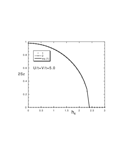
Fig.  3: When $U/t=V/t=5.0$, 2S_z as a function of $h_{x}$. The solid lines are written by eq. (1).

Fig.  4: When $U/t=V/t=5.0$, $\delta$ as a function of $h_{x}$.

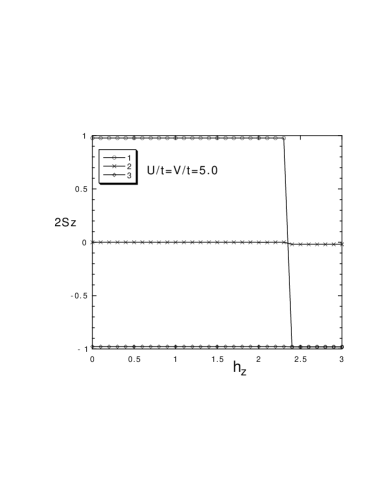
Fig.  5: When $U/t=V/t=5.0$, 2S_z as a function of $h_{z}$.

Fig.  6: When $U/t=V/t=5.0$, $\delta$ as a function of $h_{z}$.

3.2 Non-Strong coupling

We calculated the solutions as a function of $V/t$ at $U/t=1.5$. There were two solutions (($\uparrow$,$\uparrow$,$\downarrow$,$\downarrow$) and ($\uparrow$,0,$\downarrow$,0) and ($\delta$,$-\delta$,$\delta$,$-\delta$)), which are shown in Figs 7, 8 and 9. These are for the state with $2k_{\rm F}$-SDW and the coexistent state with $2k_{\rm F}$-SDW and $4k_{\rm F}$-CDW, respectively. It is found that these amplitudes of $S_{z}$ and $\delta$ are small. In the region of $0\leq V/t\leq 1.5$, the energies with these solutions are nearly the same, namely, these states are degenerate. Therefore, we analyze $h_{x}$- and $h_{z}$-dependences of $S_{z}$ and $n$ for two solutions.

We calculate the case of $U/t=V/t=1.5$ at $H\neq 0$. On using ($\uparrow$,$\uparrow$,$\downarrow$,$\downarrow$) when $H=0$, for $h_{z}$ this state is changed to ($\downarrow$,$\downarrow$,$\downarrow$,$\downarrow$) at $h_{z}^{c}=0.0155$, but, for $h_{x}$, $S_{z}$ is unchanged, which are shown in Figs. 10 and 11. This suppression for $h_{z}$ comes from Pauli paramagnetic limit since $h_{z}^{c}$ corresponds to $h_{p}\simeq 0.0125$ obtained by using eq. (12) and $E_{\rm g}/N_{\rm S}\simeq 0.0000175$ calculated at $U/t=V/t=1.5$ and $H=0$. For $h_{x}$, there is no Pauli limit, because the nesting vector of the SDW is not affected by Zeeman splitting. In Fig. 11, $S_{z}$ linearly increases as $h_{z}$ increases, which means that the paramagnetic state is stabilized by the magnetic field.

For ($\uparrow$,0,$\downarrow$,0) and ($\delta$,-$\delta$,$\delta$,-$\delta$), when the magnetic field is applied along $x$-axis, the spin and charge ordering do not change, as shown in Figs. 12 and 13. However, for $h_{z}$, both orderings of the spin and charge disappear at $h_{z}^{c}=0.0155$, which is corresponding to Pauli paramagnetic limit field, $h_{p}\simeq 0.0125$, as shown in Figs. 14 and 15. This is due to the effect of Pauli limit, too. The coexistent state of $2k_{\rm F}$-SDW and $4k_{\rm F}$-CDW with ($\uparrow$,0,$\downarrow$,0) and ($\delta$,-$\delta$,$\delta$,-$\delta$) is changed to paramagnetic state with ($\downarrow$,$\downarrow$,$\downarrow$,$\downarrow$) and (0,0,0,0). It is seen that the linear increasing of $S_{z}$ above $h_{z}^{c}$.

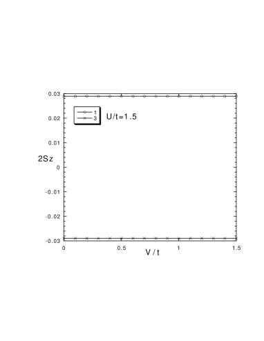
Fig.  7: By using of ($\uparrow$,$\uparrow$,$\downarrow$,$\downarrow$) at $U/t=1.5$ and $V/t=0$, $2S_{z}$ as a function of $v$ at $H=0$.

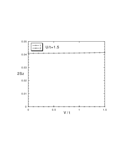
Fig.  8: By using of ($\uparrow$,0,$\downarrow$,0) at $U/t=1.5$ and $V/t=0$, $2S_{z}$ as a function of $v$ at $H=0$.

Fig.  9: By using of ($\uparrow$,0,$\downarrow$,0) at $U/t=1.5$ and $V/t=0$, $\delta$ as a function of $v$ at $H=0$.

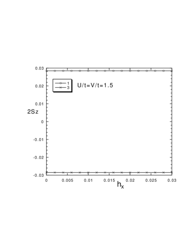
Fig.  10: When $U/t=V/t=1.5$, $2S_{z}$ as a function of $h_{x}$ by using of ($\uparrow$,$\uparrow$,$\downarrow$,$\downarrow$) at $h_{x}=0$.

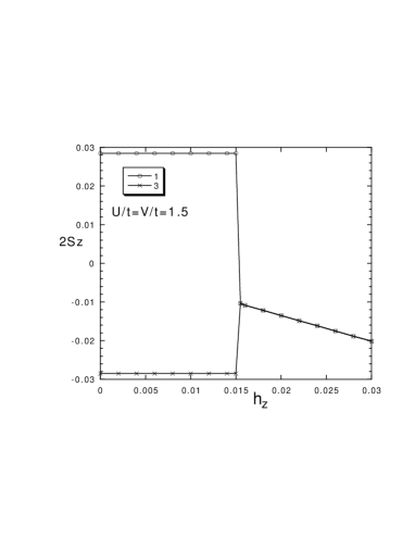
Fig.  11: When $U/t=V/t=1.5$, $2S_{z}$ as a function of $h_{z}$ by using of ($\uparrow$,$\uparrow$,$\downarrow$,$\downarrow$) at $h_{z}=0$.

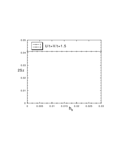
Fig.  12: When $U/t=V/t=1.5$, $2S_{z}$ as a function of $h_{x}$, by using of ($\uparrow$,0,$\downarrow$,0) at $h_{x}=0$.

Fig.  13: When $U/t=V/t=1.5$, $\delta$ as a function of $h_{x}$, by using of ($\uparrow$,0,$\downarrow$,0) at $h_{x}=0$.

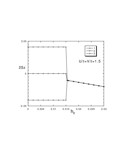
Fig.  14: When $U/t=V/t=1.5$, $2S_{z}$ as a function of $h_{z}$, by using of ($\uparrow$,0,$\downarrow$,0) at $h_{z}=0$.

Fig.  15: When $U/t=V/t=1.5$, $\delta$ as a function of $h_{z}$, by using of ($\uparrow$,0,$\downarrow$,0) at $h_{z}=0$.

3.3 Comparison with Experiments

The coexistent state with CDW and SDW is realized due to the inter-site Coulomb interaction even if the correlation between electrons is strong or not.

In the non-localized SDW system, when the magnetic field is applied parallel to the easy axis, both orderings of SDW and CDW disappear at the critical field of the Pauli paramagnetic limit. In the case of the magnetic field perpendicular to easy axis, both orderings of CDW and SDW are unchanged. In (TMTSF)₂$X$, for example, since the easy axis is $b$-axis, it is expected that when the magnetic field is applied to $b$-axis both orderings become to disorder at Pauli limit field.

On the other hand, in the localized antiferromagnetic state such as (TMTTF)₂$X$, the charge ordering is not suppressed in both cases of the magnetic field applied to parallel to and perpendicular to the easy axis. Thus, $4k_{\rm F}$-CDW may be observed from the X-ray measurement even if the magnetic field is applied to $a$, $b$ and $c$-axis. It is a means of finding whether the system is strongly correlated or not.

In (DCNQI)₂Ag, which are strongly correlated system such as (TMTTF)₂$X$, $4k_{\rm F}$-CDW has been observed at zero magnetic field.${}^{\hbox{\immediate{\bf{?}},\penalty 1000\hskip 0.91003pt plus 0.70004pt minus 0.70004pt{\bf{?}})}}$ Even under high fields, the charge ordering should be appeared.

4 Conclusions

We theoretically study the coexistent state of CDW and SDW under the magnetic field. As a result, in the case of the strongly coupling system, although the spin ordering is suppressed at high fields, the charge ordering still remains. When the coupling is not so large, the CDW and the SDW disappear at Pauli paramagnetic limit field.

These features of the coexisitent state of CDW and SDW under magnetic fields should be observed in the strongly correlated system (non-strongly correlated system) such as (TMTTF)₂$X$ and (DCNQI)₂Ag ((TMTSF)₂$X$).

5 Acknowledgment

One of the authors (K. K.) would like to thank T. Sakai for valuable discussions. K. K. was partially supported by Grant-in-Aid for JSPS Fellows from the Ministry of Education, Science, Sports and Culture. K. K. was financially supported by the Research Fellowships of the Japan Society for the Promotion of Science for Young Scientists.

References

- [1] H.Seo and H. Fukuyama: J. Phys. Soc. Jpn. 66 (1997) 1249.
- [2] N. Kobayashi and M. Ogata: J. Phys. Soc. Jpn. 66 (1997) 3356.
- [3] N. Kobayashi, M. Ogata and K. Yonemitsu: J. Phys. Soc. Jpn. 67 (1998) 1098.
- [4] S. Mazumdar, S. Rammasesha, R. Torsten Clay and David K. Campbell: Phys. Rev. Lett. 82 (1999) 1522.
- [5] For a review, see: T. Ishiguro, K. Yamaji, and G. Saito: Organic Superconductors (Springer-Verlag, Berlin 1998).
- [6] For a review, see D. Jerome: Organic Conductors ed J. P. Farges (Marcel Deckker, New York, 1994).
- [7] T. Takahashi, Y. Maniwa, H. Kawamura and G. Saito: J. Phys. Soc. Jpn. 55 (1986) 1364.
- [8] J. M. Delrieu, M. Roger, Z. Toffano and A. Moradpour: J. Phys. (Paris) 47 (1986) 839.
- [9] J. P. Pouget and S. Ravy: Synth. Met. 85 (1997) 1523.
- [10] E. Barthel, G. Quirion, P. Wzietek, D. Jerome, J. B. Christensen, M. Joregensen and K. Bechgaard: Europhys. Lett. 21 (1993) 87.
- [11] T. Nakamura, T. Nobutoki, Y. Kobayashi, T. Takahashi and G. Saito: Synth. Met. 70 (1995) 1293.
- [12] T. Nakamura, R. Kinami, Takahashi and G. Saito: Synth. Met. 86 (1997) 2053.
- [13] N. Tanemura and Y. Suzumura: J. Phys. Soc. Jpn. 65 (1996) 1792.
- [14] B. J. Klemme, S. E. Brown, P. Wzietek, G. Kriza, P. Batail, D. Jerome and J. M. Fabre: Phys. Rev. Lett. 75 (1995) 2408.
- [15] T. Mori, A. Kobayashi, Y. Sasaki and H. Kobayashi: Chem. Lett. (1982) 1923.
- [16] P. M. Grant: J. Phys. Colloq. C3 (1983) 847.
- [17] T. Mori, A. Kobayashi, Y. Sasaki and H. Kobayashi, G. Saito and H. Inokuchi: Bull. Chem. Soc. Jpn. 57 (1984) 627.
- [18] L. Ducasse, M. Abderrabba, J. Hoarau, M. Pesquer, B. Gallois and J. Gaultier: J. Phys. C19 (1986) 3805.
- [19] B. S. Shandrasekhar: Appl. Phys. Lett. 1 (1962) 7.
- [20] A. M. Clogston: Phys. Rev. Lett. 9 (1962) 266.
- [21] For study of the Pauli limit of CDW in recent, Ross H. McKenzie cond-mat/9706235.
- [22] V. Yu. Irkhin and A. A. Katanin: Phys. Rev. B58 (1998) 5509.
- [23] K. Hiraki and K. Kanoda: Phys. Rev. B54 (1996) 17276.
- [24] R. Moret, P. Erk, S. Hunig and J. U. Von Shultz: J. Phys. 49 (1988) 1925.