Correlation Effects in Multi-Band Hubbard Model and
Anomalous Properties of FeSi

In the study of a specific material among the strongly correlated electron systems, the effect of the band structures often plays a crucial role when one compares a theoretical calculation to the experiments. Use of a simple theoretical model might not capture the salient features of the material. Development of a theoretical method that is capable of taking proper account of the realistic features of the material is necessary. We report our recent approach to the study of the anomalous properties of FeSi in such direction.

FeSi is well known for more than thirty years and a number of studies from various aspects have been done, stimulated by the fascinating physical properties. The early study by Jaccarino et al.${}^{\hbox{\immediate{\bf{?}})}}$ showed that the susceptibility is much enhanced over the value expected from the band paramagnetism at finite temperatures and has a broad peak at about 500 K. It was also reported that the specific heat seems to have an anomalous enhancement at about 250 K. These behaviors were explained by a band model with an energy gap, but unphysically narrow bands were necessary, so that this difficulty has attracted interests of many researchers. From the conductivity measurements, FeSi is an insulator at low temperatures but shows metallic behavior at room temperature. To explain these unusual properties of FeSi, several theoretical approaches have been proposed, but the most successful one is the spin fluctuation scenario by Takahashi and Moriya.${}^{\hbox{\immediate{\bf{?}})}}$ It explains the anomalous magnetic property of FeSi and their idea of the thermally induced magnetic moment was confirmed by the neutron scattering experiment.${}^{\hbox{\immediate{\bf{?}})}}$

The recent optical studies,${}^{\hbox{\immediate{\bf{?}},\penalty 1000\hskip 0.91003pt plus 0.70004pt minus 0.70004pt{\bf{?}},\penalty 1000\hskip 0.91003pt plus 0.70004pt minus 0.70004pt{\bf{?}},\penalty 1000\hskip 0.91003pt plus 0.70004pt minus 0.70004pt{\bf{?}})}}$ however, revealed the unusual properties of FeSi again. Schlesinger et al. reported that the gap of about 60 meV ($\sim$700 K) opened at low temperatures is filled and almost closed at room temperature (about 250$\sim$300 K), which they attributed to the correlation effect. The following experiments also reported the evidence of the correlation effects at low temperatures.${}^{\hbox{\immediate{\bf{?}},\penalty 1000\hskip 0.91003pt plus 0.70004pt minus 0.70004pt{\bf{?}},\penalty 1000\hskip 0.91003pt plus 0.70004pt minus 0.70004pt{\bf{?}},\penalty 1000\hskip 0.91003pt plus 0.70004pt minus 0.70004pt{\bf{?}})}}$ In these contexts, Aeppli and Fisk${}^{\hbox{\immediate{\bf{?}})}}$ suggested that FeSi can be viewed as a Kondo insulator or a strongly correlated insulator.

Kondo insulators have been found in the f-electron systems and typical examples are YbB₁₂${}^{\hbox{\immediate{\bf{?}})}}$ and Ce₃Bi₄Pt₃${}^{\hbox{\immediate{\bf{?}})}}$ and so on. They have correlated f-bands and small energy gaps at low temperatures. Although there are many similarities among FeSi and these materials, the correlation in FeSi may not be so strong. However, the same physics can be recognized both in FeSi and Kondo insulators, if one reexamines the experimental data carefully. From this aspect, Fu and Doniach${}^{\hbox{\immediate{\bf{?}})}}$ proposed an extended Hubbard model with two mixed conduction bands, which is based on their band calculation${}^{\hbox{\immediate{\bf{?}})}}$ for FeSi, and confirmed the importance of the correlation effects in physical quantities. Their calculation, however, seems to include some errors about the treatment of the self-energies. Therefore, we reinvestigated this model carefully and calculated the correlation effects in more correct way,${}^{\hbox{\immediate{\bf{?}})}}$ and confirmed that the correlation effects do play important roles, but the shape of the spectrum in the optical conductivity did not coincide with the experimental data, because of the use of the too simple model Hamiltonian.

Therefore in the present report, we use an extended two-band Hubbard model with the density of states obtained from the band calculation, and attempt to explain the low temperature anomalies of FeSi observed in the optical conductivity${}^{\hbox{\immediate{\bf{?}})}}$ and the specific heat consistently.

The band calculations${}^{\hbox{\immediate{\bf{?}},\penalty 1000\hskip 0.91003pt plus 0.70004pt minus 0.70004pt{\bf{?}},\penalty 1000\hskip 0.91003pt plus 0.70004pt minus 0.70004pt{\bf{?}},\penalty 1000\hskip 0.91003pt plus 0.70004pt minus 0.70004pt{\bf{?}},\penalty 1000\hskip 0.91003pt plus 0.70004pt minus 0.70004pt{\bf{?}})}}$ for FeSi predict that the ground state is a band insulator and a recent calculation${}^{\hbox{\immediate{?})}}$ reproduces the gap size close to the observed one. Therefore, we start from the band insulator model, which consists of two Hubbard bands for d-electrons as follows.

$$H= \sum_{ij\sigma}(t^{1}_{ij}c_{i1\sigma}^{\dagger}c_{j1\sigma}+t^{2}_{ij}c_{2i\sigma}^{\dagger}c_{2j\sigma})$$ (1)

$$+ U\sum_{i}(n_{i1\uparrow}n_{i1\downarrow}+n_{i2\uparrow}n_{i2\downarrow})$$ (2)

$$+ U_{2}\sum_{i}(n_{i1\uparrow}n_{i2\downarrow}+n_{i2\uparrow}n_{i1\downarrow})$$ (3)

$$+ U_{3}\sum_{i}(n_{i1\uparrow}n_{i2\uparrow}+n_{i2\downarrow}n_{i1\downarrow})$$ (4)

$$- J\sum_{i}(c_{i1\uparrow}^{\dagger}c_{i1\downarrow}c_{i2\downarrow}^{\dagger}c_{i2\uparrow}+c_{i2\uparrow}^{\dagger}c_{i2\downarrow}c_{i1\downarrow}^{\dagger}c_{i1\uparrow}),$$ (5)

where the $c^{\dagger}_{ia\sigma}(c_{ia\sigma})$ creates (destroys) an electron on site $i$ in band $a=$1, 2 with spin $\sigma$. The tight binding parameters $t^{a}_{ij}$ should be fitted to the band calculation and $U$, $U_{2}$, $U_{3}$ and $J$ denote the Coulomb and exchange interactions.

Since one can expect that the optical conductivity spectrum reflects the structure of the quasi-particle density of states (DOS) of a system, we use the DOS obtained from the band calculation for FeSi by Yamada et al.${}^{\hbox{\immediate{?})}}$ for the initial DOS so as to enable detailed comparison with the experiment.

Furthermore, we start from the following general expression of the current operator,

$$j=e\sum_{\sigma,{\bf k}}\sum_{mm^{\prime}}v^{mm^{\prime}}_{\bf k}c^{\dagger}_{m{\bf k}}c_{m^{\prime}{\bf k}},$$ (6)

where $m$ denotes the band indices and derive the convenient expression for the optical conductivity. For simplicity, we set the intra- and interband contributions to be equal ($v^{mm^{\prime}}_{\bf k}=v_{\bf k}$). Moreover, we assume that the momentum conservation is violated in real systems by some defects and phonon-assisted transitions. Therefore, using the linear response theory, we consider the current-current correlation function as below,

$$K(i\omega_{n}) = \int^{\beta}_{0}d\tau e^{i\omega_{n}\tau}\sum_{mm^{\prime}}\sum_{{\bf kk^{\prime}}\sigma\sigma^{\prime}}v_{\bf k}v_{\bf k^{\prime}}$$ (12)

$$\!\!\!\times<T_{\tau}c^{\dagger}_{m{\bf k}\sigma}(\tau)c_{m{\bf k}\sigma}(\tau)c^{\dagger}_{m^{\prime}{\bf k^{\prime}}\sigma^{\prime}}(0)c_{m^{\prime}{\bf k^{\prime}}\sigma^{\prime}}(0)>$$

$$\!\!\!\!\!\!\!\!\!\!\!\!\!\!\!\!\!\!\!\!\!\!\!\!\simeq-\frac{1}{\beta}\sum_{mm^{\prime}}\sum_{l}\sum_{{\bf kk^{\prime}}\sigma}v_{\bf k}v_{\bf k^{\prime}}{\cal G}^{m}_{{\bf k}\sigma}(i\nu_{l}){\cal G}^{m^{\prime}}_{{\bf k}^{\prime}\sigma}(i\nu_{l}+i\omega_{n})$$

$$\!\!\!\!\!\!\!\!\!\!\!\!\!\!\!\!\!\!\!\!\!\!\!\!\times[\delta_{\bf kk^{\prime}}+\Gamma_{\bf kk^{\prime}}^{mm^{\prime}\sigma}(i\nu_{l};i\omega_{n}){\cal G}^{m}_{{\bf k^{\prime}}\sigma}(i\nu_{l}){\cal G}^{m^{\prime}}_{{\bf k}\sigma}(i\nu_{l}+i\omega_{n})],$$

where $\Gamma_{\bf kk^{\prime}}^{mm^{\prime}\sigma}(i\nu_{l};i\omega_{n})$ denotes the vertex function, and set $[\dots]$ constant. For the present case, this leads to the following expression for the optical conductivity,

$$\sigma(\omega,T) = \frac{\pi(ev)^{2}}{\hbar}\sum_{\sigma}\int^{\infty}_{-\infty}d\nu\frac{f(\nu)-f(\nu+\omega)}{\omega}$$ (14)

$$\times[\rho^{\sigma}_{1}(\nu)+\rho^{\sigma}_{2}(\nu)][\rho^{\sigma}_{1}(\nu+\omega)+\rho^{\sigma}_{2}(\nu+\omega)],$$

where $\rho^{\sigma}_{a}(\nu)$ denotes the DOS for the band $a$. This joint-DOS-like form for the optical conductivity is simple but convenient for the present case. We set $(ev)^{2}/\hbar=1$ for simplicity.

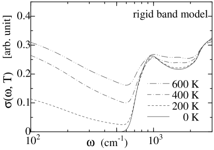
Fig.  1: Fig. 1 Calculated optical conductivity within the Hartree-Fock approximation or a rigid band model.

Firstly, we show the optical conductivity obtained from the Hartree-Fock approximation (HFA) or a rigid band model in Fig. 1. The used DOS is displayed in Fig. 2 by the solid line for $T=0$. The DOS is independent of the temperature within HFA. At 0 K, only the interband contribution survives and reproduces the shape of the spectrum of the experiment at 4 K in Fig. 3. Therefore, the band calculation by Yamada et al.${}^{\hbox{\immediate{?})}}$ seems to give a good result about the whole structure of the DOS at $T=0$ but with a slightly smaller gap size (see the comparison with the experiment below). Within the rigid band model, however, since the gap is filled only with the intraband (Drude) contribution, the temperature variation is monotonous and the spectrum does not become flat at a temperature of the order of the gap size. This disagreement was shown by Fu et al. first. Ohta et al.${}^{\hbox{\immediate{?})}}$ also calculated the optical conductivity in the joint-DOS form from their band calculation, but the flat part of the optical conductivity spectrum within the gap could not be reproduced. Therefore, the rigid band model is not sufficient to explain the experiments.

Next, we investigate the correlation effect in the low energy and low temperature region of this model. Therefore we calculate the correlation effect by the self-consistent second-order perturbation theory (SCSOPT) combined with the local approximation. The second-order self-energies are given by

$$\Sigma_{1}^{(2)\sigma}(\omega) = \int\!\!\!\int\!\!\!\int^{\infty}_{-\infty}d\varepsilon_{1}d\varepsilon_{2}d\varepsilon_{3}$$ (23)

$$[U^{2}\rho_{1}^{-\sigma}(\varepsilon_{1})\rho_{1}^{\sigma}(\varepsilon_{2})\rho_{1}^{-\sigma}(\varepsilon_{3})$$

$$+U_{2}^{2}\rho_{2}^{-\sigma}(\varepsilon_{1})\rho_{1}^{\sigma}(\varepsilon_{2})\rho_{2}^{-\sigma}(\varepsilon_{3})$$

$$+U_{3}^{2}\rho_{2}^{\sigma}(\varepsilon_{1})\rho_{1}^{\sigma}(\varepsilon_{2})\rho_{2}^{\sigma}(\varepsilon_{3})$$

$$+J^{2}\rho_{2}^{-\sigma}(\varepsilon_{1})\rho_{2}^{\sigma}(\varepsilon_{2})\rho_{1}^{-\sigma}(\varepsilon_{3})]$$

$$\times \frac{f(-\varepsilon_{1})f(\varepsilon_{2})f(\varepsilon_{3})+f(\varepsilon_{1})f(-\varepsilon_{2})f(-\varepsilon_{3})}{\omega+\varepsilon_{1}-\varepsilon_{2}-\varepsilon_{3}+{\rm i}\delta},$$ (25)

$$\Sigma_{2}^{(2)\sigma}(\omega) = (1\leftrightarrow 2),$$ (26)

where $\rho_{a}^{\sigma}(\omega)=-(1/\pi){\rm Im}G_{a}^{\sigma}(\omega+{\rm i}\delta)$ and

$$G_{a}^{\sigma}(\omega) =\frac{1}{N}\sum_{\bf k}G_{a}^{\sigma}({\bf k},\omega)$$ (28)

$$=\int^{\infty}_{-\infty}d\varepsilon\rho^{0\sigma}_{a}(\varepsilon)\frac{1}{\omega-\varepsilon-\Sigma^{(2)\sigma}_{a}(\omega)}.$$

Here, $N$ is the number of sites, $f(\varepsilon)$ the Fermi function and $\rho^{0\sigma}_{a}(\varepsilon)$ the DOS of band $a$ for the non-interacting case. To make numerical calculation easy, we take $\delta$ finite ($\delta=10^{-7}$) in eq. (28) and convert these equations with the transformations${}^{\hbox{\immediate{\bf{?}})}}$

$$A_{a}^{\sigma}(\tau) = \int^{\infty}_{-\infty}d\epsilon e^{-{\rm i}\tau\varepsilon}\rho_{a}^{\sigma}(\varepsilon)f(\varepsilon),$$ (29)

$$B_{a}^{\sigma}(\tau) = \int^{\infty}_{-\infty}d\epsilon e^{-{\rm i}\tau\varepsilon}\rho_{a}^{\sigma}(\varepsilon)f(-\varepsilon).$$ (30)

These equations have to be solved self-consistently. In this paper, we set $U_{2}=U-J$ and $U_{3}=U-2J$ in order to reduce the number of parameters. In this case, the Hamiltonian is rotationally invariant in spin and real spaces if the two bands are degenerate.${}^{\hbox{\immediate{\bf{?}})}}$

In the following results, $U=0.5$ eV and $J=0.35U$ are chosen so as to reproduce the shape and the temperature dependence of the optical conductivity spectrum. The solid line for $T=0$ in Fig. 2 indicates the initial DOS at 0 K, and the correlation effect is absent except the Hartree-Fock contribution since the band 1 is filled and the band 2 is empty.

Note that the gap in the DOS is widened by 16 $\%$ so as to reproduce the shape of the spectrum of the optical conductivity at 4 K in the experiment, which does not change the essence of the following result. Then, the gap size ($E_{g}$) of $75$ meV is obtained if the steepest parts of the DOS at the both sides of the gap are extrapolated and the tails are neglected. (If we regard the gap as the region inside the tails of the gap edge, we obtain 60 meV.) The band 1 and 2 in our Hamiltonian correspond to the upper and lower part of the DOS with respect to the Fermi level ($E_{F}=0$) as is seen in Fig. 2, where we introduce a cut off for each band so as to include one state per spin in each band. Then the band width for the band 1 and 2 are about 0.56 eV and about 0.85 eV, respectively. Although the DOS is asymmetric, the chemical potential is fixed at $\omega=0$ and assumed to be temperature independent. One can see in Fig. 2 that the correlation is introduced at finite $T$ through the thermally excited electrons and holes and the gap existing at 0 K is almost filled up at the temperature of the order of its size, which results in the temperature variation of the interband contribution of the optical conductivity (see below).

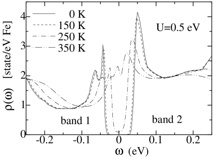
Fig.  2: The temperature dependence of the quasi-particle DOS and the initial DOS obtained from the band calculation(Ref. 26) at $T=0$. At finite $T$, the DOS is strongly temperature dependent due to the correlation effects.

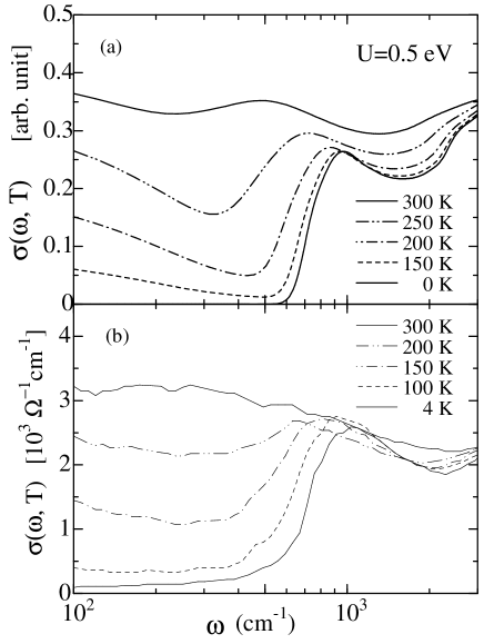
Fig.  3: (a)The temperature dependence of the optical conductivity calculated with the eq. (14). (b)The experimental data from Ref. 11. The peaks due to phonons observed in the gap are omitted.

In Fig. 3(a), the temperature variation of the optical conductivity calculated from the temperature-dependent DOS in Fig. 2 is shown. In our calculation (Fig. 3(a)), the gap is almost filled up at 300 K as well as the rapid increase in the gap region from 150 to 300 K is seen. This is consistent with the experiment (Fig. 3(b)), where the gap is filled rapidly from 100 K to 300 K. Reflecting the correlation effects, the peak at the gap edge shifts to lower frequency region, as is seen in the experiment. In our calculation, however, there are dips between the Drude and the interband contributions in contrast to the experiment. This may be caused by the simplification in deriving eq. (14). However, the almost flat spectrum is obtained at 300 K, which comes from the temperature dependence of the interband contribution.

We also calculate the temperature variation of the specific heat with the same parameters as in the optical conductivity. Starting from the equation of motion,${}^{\hbox{\immediate{\bf{?}})}}$ we obtain the following expression for the total energy per site:

$$E = \frac{1}{2}\sum_{\sigma}\int^{\infty}_{-\infty}d\omega f(\omega)\left[\omega\{\rho^{\sigma}_{1}(\omega)+\rho^{\sigma}_{2}(\omega)\}\right.$$ (32)

$$+\frac{1}{N}\sum_{\bf k}\left.\{\varepsilon^{1}_{\bf k}\rho^{\sigma}_{1}({\bf k},\omega)+\varepsilon^{2}_{\bf k}\rho^{\sigma}_{2}({\bf k},\omega)\}\right],$$

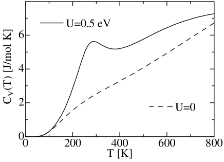
Fig.  4: Calculated specific heat using the same parameter as in Fig. 3(a).

where $\varepsilon^{1}_{\bf k}$ ($\varepsilon^{2}_{\bf k}$) is the Fourier transformation of $t^{1}_{ij}$ ($t^{2}_{ij}$). The specific heat can be calculated from the numerical differentiation of the energy as $C_{V}=(\partial E/\partial T)_{V}$. The difference between the cases with $U=0$ and $0.5$ eV in Fig. 4 indicates the contribution from the correlation effect, which results in a peak of about 4 J/K mol at about 250 K, and explains the “anomalous” contribution ($\sim$6 J/K mol) in the specific heat at about 250 K reported by Jaccarino et al.${}^{\hbox{\immediate{?})}}$ Note that they evaluated the anomaly by subtracting the specific heat of CoSi after the normal electronic contributions $\gamma_{\rm FeSi}$ and $\gamma_{\rm CoSi}$ are removed, respectively. In the above calculations, we confirmed that the correlation effect is essential to explain the temperature dependence of the optical conductivity and the specific heat in FeSi. At higher temperatures or for magnetic properties, however, it is also important to take the spin fluctuations ${}^{\hbox{\immediate{?},\penalty 1000\hskip 0.91003pt plus 0.70004pt minus 0.70004pt{\bf{?}})}}$ into account.

The self-consistent renormalization (SCR) theory of spin fluctuations has succeeded in describing the itinerant magnetism and the quantum critical phenomena with a small number of parameters.${}^{\hbox{\immediate{\bf{?}})}}$ On the other hand, the dynamical mean field theory (DMFT) is one of the most powerful schemes to take account of the strong local correlation. One of the authors has proposed a new and practical scheme that unifies DMFT and SCR in a microscopic way.${}^{\hbox{\immediate{?})}}$ Application of this theory to FeSi may improve the present calculation towards the inclusion of the effects of spin fluctuations at finite temperatures and the intermediate coupling.

References

- [1] V. Jaccarino, G. K. Wertheim, J. H. Wernick, L. R. Walker and S. Arajs: Phy. Rev. 160 (1967) 476.
- [2] Y. Takahashi and T. Moriya: J. Phys. Soc. Jpn. 46 (1979) 1451;Y. Takahashi, J. Phys.: Cond. Matter 9 (1997) 2593.
- [3] G. Shirane, J. E. Fisher, Y. Endoh and K. Tajima: Phys. Rev. Lett. 59 (1987) 351; K. Tajima, Y. Endoh, J. E. Fisher and G. Shirane: Phys. Rev. B 38 (1988) 6954.
- [4] Z. Schlesinger, Z. Fisk, Hai-Tao Zhang, M. B. Maple, J. F. DiTusa and G. Aeppli: Phys. Rev. Lett. 71 (1993) 1748.
- [5] H. Ohta, S. Kimura, E. Kulatov, S. V. Halilov, T. Nanba, M. Motokawa, M. Sato and K. Nagasawa: J. Phys. Soc. Jpn. 63 (1994) 4206.
- [6] S. Paschen, E. Felder, M. A. Chernikov, L. Degiorgi, H. Schwer, H. R. Ott, D. P. Young, J. L. Sarrao and Z. Fisk: Phys. Rev. B 56 (1997) 12916.
- [7] A. Damascelli, K. Schulte, D. van der Marel, M. Fäth and A. A. Menovsky: Physica B 230-232 (1997) 787.
- [8] T. Saitoh, A. Sekiyama, T. Mizokawa, A. Fujimori, K. Ito, H. Nakayama and M. Shiga: Solid State Commun. 95 (1995) 307.
- [9] M. A. Chernikov, L. Degiorgi, E. Felder, S. Paschen, A. D. Bianchi, H. R. Ott, J. L. Sarrao, Z. Fisk and D. Mandrus: Phys. Rev. B 56 (1997) 1366.
- [10] M. Fäth, J. Aarts, A. A. Menovsky, G. J. Nieuwenhuys and J. A. Mydosh: Phys. Rev. B 58 (1995) 15483.
- [11] J. F. DiTusa, K. Friemelt, E. Bucher, G. Aeppli and A. P. Ramirez: Phys. Rev. B 58 (1998) 10288.
- [12] G. Aeppli and Z. Fisk: Comments Condens. Matter Phys. 16 (1992) 155.
- [13] M. Kasaya: J. Mag. Magn. Mater. 47 & 48 (1985) 429.
- [14] M. F. Hundley, P. C. Canfield, J. D. Thompson, Z. Fisk and J. M. Laurence: Phys. Rev. B 42 (1990) 4862.
- [15] C. Fu and S. Doniach: Phys. Rev. B 51 (1995) 17439.
- [16] C. Fu, M. P. C. M. Krijn and S. Doniach: Phys. Rev. B 49 (1994) 2219.
- [17] K. Urasaki and T. Saso: Phys. Rev. B 58 (1998) 15528.
- [18] K. Urasaki and T. Saso: J. Phys. Soc. Jpn. 68 (1999) 3477.
- [19] L. F. Mattheiss and D. R. Hamann: Phys. Rev. B 47 (1993) 13114.
- [20] T. Jarlborg: Phys. Rev. B 51 (1995) 11106.
- [21] V. R. Galakhov, E. Z. Kurmaev, V. M. Cherkashenko, Yu M. Yarmoshenko, S. N. Shamin, A. V. Postnikov, St Uhlenbrock, M. Neumann, Z. W. Lu, B. M. Klein and Zhu-Pei Shi: J. Phys.: Condens. Matter 7 (1995) 5529.
- [22] E. Kulatov and H. Ohta: J. Phys. Soc. Jpn. 66 (1997) 2386.
- [23] H. Yamada, K. Terao, H. Ohta, T.Arioka and E. Kulatov: J. Phys.: Condens. Matter 11 (1999) L309.
- [24] R. H. Parmenter: Phys. Rev. B 8 (1973) 1273.
- [25] E. Müller-Hartmann: Z. Phys. 76 211 (1989).
- [26] A. L. Fetter and J. D. Walecka, Quantum Theory of Many-Particle Systems (McGraw Hill, 1971).
- [27] T. Saso: J. Phys. Soc. Jpn 68 (1999) 3941.
- [28] T. Moriya, ”Spin fluctuations in Itinerant Electron Magnetism” (Springer, 1985).