I General Discussion

The purpose of this article is to analyze the dependence of the energy of an elementary excitation on the strength of the confinement potential, which exists in a planar semiconductor heterostructure. Due to the fascinating technological progress in the field of man-made structures, it has become possible to fabricate e.g. quantum wells of a widely varying shape. It is an interesting theoretical task to discuss the excitation spectrum of such semiconductor structures as function of the tunable parameters, such as well width, well height, etc.. Concerning the excitations of interest, we concentrate on particle-phonon systems, the particles being electrons or holes. The simplest example is that of a single polaron, that is an electron, coupled to a certain branch of lattice vibrations. Another example is that of a polaronic exciton, that is an electron-hole pair, coupled to phonons. Whereas the latter one is important to characterize optical properties, the former one has direct implications for the transport behavior of the materials of interest.

We assume that the interface(s)-induced confinement can be mimicked by a simple potential $V_{n}(z_{n})$, $n$ being the particle number, $z_{n}$ the corresponding coordinate (the growth direction of the heterostructure will always be assumed as $z$-direction). Explicit forms of $V_{n}(z_{n})$ may be rectangular wells, parabolas etc.. In addition, we suppose translation invariance to hold within the $xy$-plane. We remark that effects as surface roughness would destroy this property and could lead to the appearanc of new phenomena (e.g. localized states).

In the following equation, we define the class of models under discussion:

$$H: = \frac{1}{2}\sum_{n=1}^{N}{\bf{p}}_{n}{m_{n}}^{-1}{\bf{p}}_{n}+U({\bf{r}}_{1},..,{\bf{r}}_{N})+$$ (2)

$$\sum_{\bf{k}}\hbar\,{\omega}_{\bf{k}}\,a_{\bf{k}}^{+}a_{\bf{k}}+\frac{1}{\sqrt{V}}\sum_{n=1}^{N}\sum_{\bf{k}}\left(g_{\bf{k},n}\,e^{\,i\,\bf{k}\bf{r}_{n}}\,a_{\bf{k}}+h.c.\right)$$

$$= :H_{el}+H_{ph}+H_{int}.$$ (3)

The nomenclature is self explaining. The quantity $U(\bf{r}_{1},\bf{r}_{2})$ is to contain the confinement potentials as well as the particle interaction:

$$U({\bf{r}}_{1},..,{\bf{r}}_{N}):=\sum_{n=1}^{N}\,V_{n}(z_{n})+\frac{1}{2}\sum_{\begin{array}[]{l}n,n^{\prime}=1,\\[-5.69054pt] n\neq n^{\prime}\end{array}}^{N}\,V_{n,n^{\prime}}({\bf{r}}_{n},{\bf{r}}_{n^{\prime}}),$$ (4)

where $V_{n,n^{\prime}}$ has to be calculated as potential energy of particle $n$, exposed to the electrostatic potential of particle $n^{\prime}$. Because of the boundary conditions, $V_{n,n^{\prime}}({\bf{r}}_{n},{\bf{r}}_{n^{\prime}})$ itself is not translation invariant (see e.g. Ref. [3]). The particle-phonon coupling is of Fröhlich type. The most prominent example to be used here is that of a coupling to (LO)-phonons.

The model has two relevant limiting cases, which should be reproduced by any theory. Let the maximum of the well widths be $L$ and the minimum $L^{\prime}$. If $L^{\prime}$ tends to infinity, the confinement is irrelevant and the energy spectrum of $H$ is that of a three-dimensional well-material excitation. If $L$ tends to zero, the (finite height) well is irrelevant, leaving us with the spectrum of a three-dimensional barrier-material excitation. The behaviour for intermediate values of the well widths can qualitatively be discussed as follows. Varying $L,L^{\prime}$ from sufficiently large values to smaller ones, the binding energy should increase due to the higher Coulomb correlation (for instance, the reader should recall that the energy of the two-dimensional hydrogen ground state is four times larger than that of a three-dimensional one). When $L,L^{\prime}$ become smaller and smaller, the ground-state wave function will more and more effectively tunnel into the barrier material — the energy approaches the barrier limit.

Thus, we might expect a maximum of the binding energy to appear at intermediate values of $L,L^{\prime}$. It was a controversely discussed question whether or not this maximum appears at relevant (that is not too small) values of $L$. The answer to this question might be not the same for different systems.

II Polarons

The physics of polarons, confined to quantum wells, passed a few stages, and it is not possible to present here even a brief list of references. In particular, it was found that different phonon modes contribute to the polaron binding energy — confined bulk 2phonons inside the well, interface phonon mode and half-space bulk phonon mode in the barrier. We cite only papers[4, 5] concerning polarons confined to a finite rectangular potential (one layer heterostructure) where contribution of all phonon modes were taken into account. Anyway, there are problems to be addressed while dealing with multilayered heterostructures. Namely, we have to answer the following questions:

1) How to deal with multilayered heterostructures? The total number of phonon modes becomes too large to make numerical calculations even with modern computers. Besides, a multilayered heterostructure can generate a confining potential of rather complicated form, not only the rectangular one.

2) How to deal with mass- and dielectric mismatches in different layers? The polaron effective mass $m(z)$, the electron-phonon coupling constant $\alpha(z)$ and the phonon dispersion law do depend on a layer, that is, on the electron position. To glue solutions in different layers seems to be a cumbersome job.

To tackle these problems we suggest specific approximations, which will briefly be indicated here.

• A multilayered $GaAs/Al_{x}Ga_{1-x}As$ heterostructure is considered as an effective medium. Its mean parameters are to be defined by averaging over different layers according to the way they enter the Hamiltonian.
  

• The bulk phonon mode only inhabits an effective medium with mean characteristics.

We specify the electronic part of the Hamiltonian:

$$H_{el}=H_{el,\parallel}+H_{el,\perp}={\vec{p}_{\parallel}^{\,2}\over 2m}+{p_{z}^{\,2}\over 2m}+V(z),$$ (5)

The mean electron band mass $m$ is defined by the equation

$$H_{el,\perp}\psi_{1}=E_{1}\psi_{1},\qquad{1\over m}=\int\limits_{-\infty}^{\infty}dz\,{|\psi_{1}(z)|^{2}\over m(z)},$$ (6)

where $\psi_{1}(z),E_{1}$ are the ground state wave function and the energy for the electron motion in $z$ direction. As $\psi_{1}$ and $E_{1}$ depend on $m$, we actually have the system of two equations (6) to calculate the mean band mass $m$.

The free LO-phonon Hamiltonian reads as follows:

$$H_{ph}=\hbar\omega_{\mbox{LO}}\sum\limits_{\vec{k}}a^{{\dagger}}_{\vec{k}}a_{\vec{k}}\ \ ,\qquad\omega_{\mbox{LO}}=\int\limits_{-\infty}^{\infty}dz\,\omega(z)\,|\psi_{1}(z)|^{2}.$$ (7)

As $m$ is found already, we define here the mean phonon frequency $\omega_{\mbox{LO}}$. Note that in this paper we are not interested in processes of emission, absorption or scattering of phonons. Instead we concentrate on virtual phonons in a cloud around an electron. Subsequently, the properties of the effective phonons do depend on the position of the electron as it follows from Eq. (7).

In the same way we define the effective electron-phonon interaction Hamiltonian in the standard Fröhlich form with the mean Fröhlich coupling constant $\alpha$:

$$\sqrt{\alpha}=\int\limits_{-\infty}^{\infty}dz\,|\psi_{1}(z)|^{2}\,{\omega(z)\over\omega_{\mbox{LO}}}\left(\alpha(z)\sqrt{m\omega_{\mbox{LO}}\over m(z)\omega(z)}\right)^{1/2}.$$ (8)

Evidently, this model belongs to the class defined in Eq. (2) As examples we studied 1) a one-layer heterostructure described by a rectangular confining potential

$$V(z)=\left\{\begin{array}[]{ll}0,&|z|\leq L/2\\ V_{0},&|z|>L/2\end{array}\right..$$ (11)

(the $z$-dependence of the masses and dielectric parameters is completely analogous) and 2) a multilayered heterostructure corresponding to the Rosen-Morse potential

$$V(z) = V_{0}\,{\rm tanh}^{2}\left({z\over L_{RM}}\right).$$ (12)

We use perturbation theory in powers of $\alpha$ for both potentials, but in the first case we perform the summation over all virtual states while in the case of the Rosen-Morse potential the Green function (see [6, 7]) can be used. To compare results for the Rosen-Morse and the rectangular potentials, an effective width $L$ of the Rosen-Morse potential has to be found. We define it as the width of a rectangular potential of the same height $V_{0}$ with the same ground-state energy. The dependence $L(L_{RM})$ can then be calculated. The parametrization for experimental data concerning $GaAs/Al_{x}Ga_{1-x}As$ heterostructure is based on the results reported in Ref. [8] with some modifications, which are discussed in our paper[9]. Actually we use the dependence of the parameters on the $Al$ mole fraction $x$ which depends in turn on the coordinate $z$ via the relation $V(z)=600\cdot(1.155x+0.37x^{2})\ {\rm meV}$. The confining potential $V(z)$ being given, we know the dependence $x(z)$ and, subsequently, the values of the parameters $\alpha,m,\omega$ at each point of the heterostructure which are averaged then following Eqs. (6), (7) and (8).

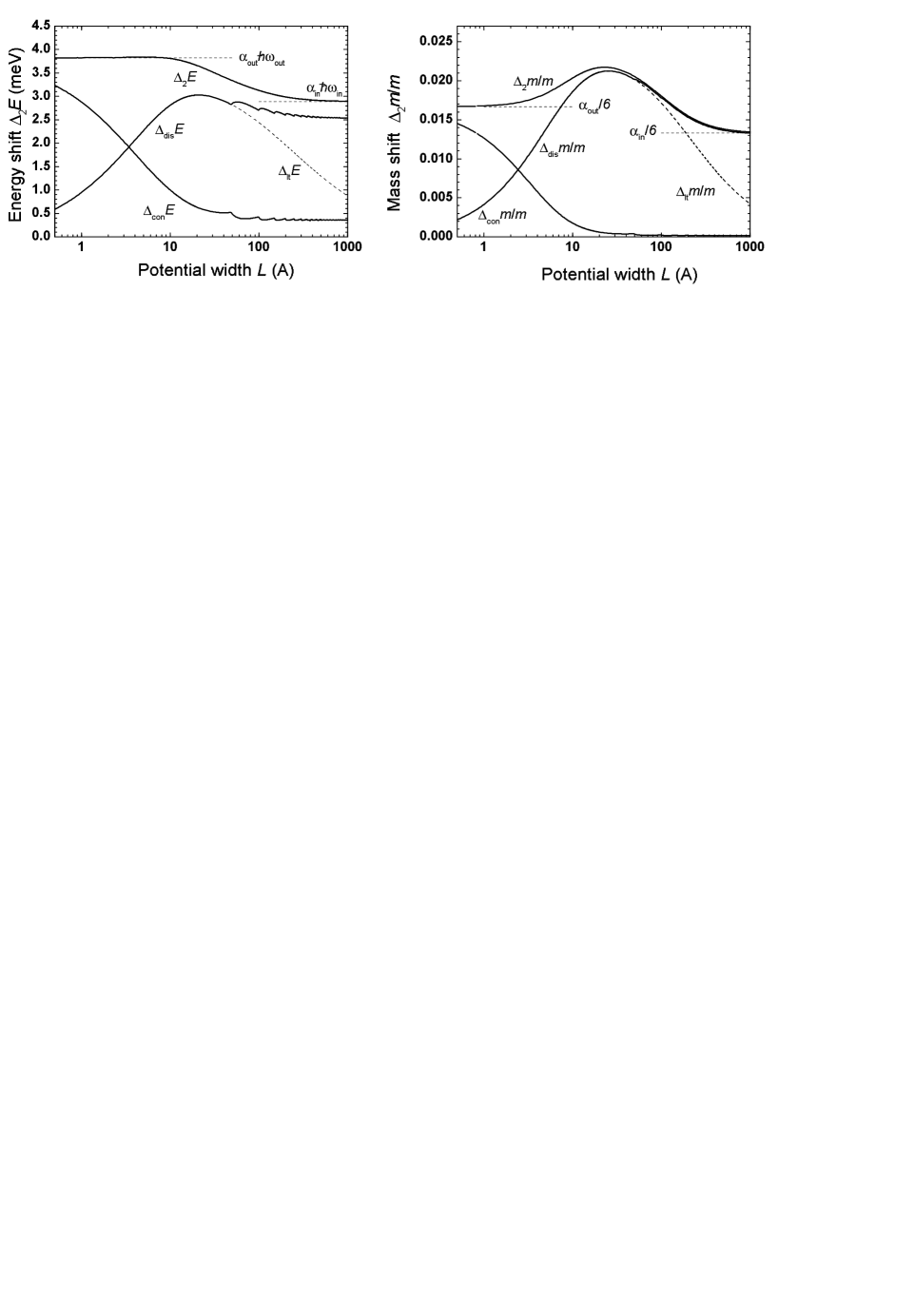
FIG. 1.: The polaron binding energy and the effective mass in the rectangular potential. Contributions of the discrete $\Delta_{dis}E\ (\Delta_{dis}m/m)$ and continuous $\Delta_{con}E\ (\Delta_{con}m/m)$ spectrum are shown as well as the so called leading term approximation $\Delta_{lt}E\ (\Delta_{lt}m/m)$ when only the ground state is taken into account as an intermediate virtual state (dashed line).

The polaron energy and effective mass are calculated for $x=0.3$. Peaks are found for the effective mass at some potential widths, while the energy demonstrates rather a smooth behavior between the correct 3D-limits as is seen in Fig. 1. As to the Rosen-Morse potential, the results are presented in Fig. 2 together with those for the rectangular potential of the corresponding effective width. One can see an excellent coincidence of the results obtained within the different techniques; clearly, this fact increases their reliability. A comparison is also made with the results of the papers[4, 5], and the details are discussed in our paper[9].

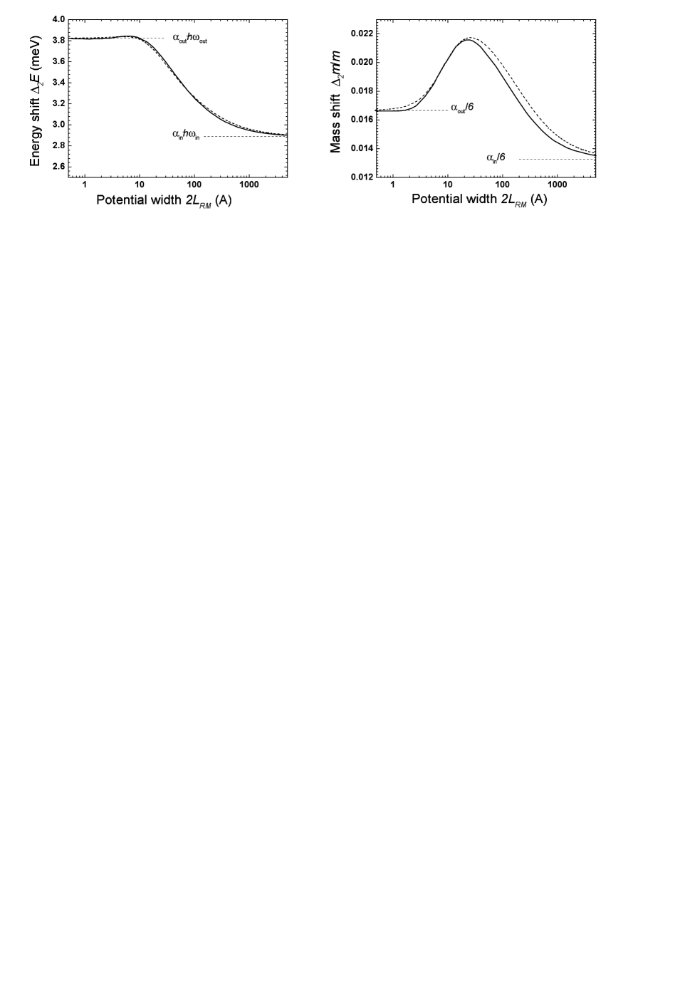
FIG. 2.: Our results for the Rosen-Morse potential in comparison with these for the rectangular potential (dashed line) of the same effective width $L(L_{RM})$.

III Excitons

Sampling the previous literature, most work has been done on rectangular quantum wells with confinement potentials of type (11). The electron-hole potential can be calculated as indicated above and was given e.g. in Ref. [3].

To treat eigenvalue problems as the present one, we use tractable decompositions of the Hamiltonian to generate lower bounds for the ground-state energy. The basic idea is as follows: Assume we study the Hamiltonian $H=p_{z}^{2}/2m+V_{1}(z)+V_{2}(z)$ to find its ground-state energy $E$. Then we use the decomposition

$$H_{1}=x{p_{z}^{2}\over 2m}+V_{1}(z),\quad H_{2}=(1-x){p_{z}^{2}\over 2m}+V_{2}(z),\qquad 0\leq x\leq 1.$$ (13)

If $E_{1}(x),E_{2}(x)$ are the corresponding ground-state energies of $H_{1},H_{2}$, then a lower bound for $E$ is: $E\geq\max_{x}(E_{1}(x)+E_{2}(x))$.

Upper bounds are produced by variational methods: The trial wave-function used in our calculations had the form:

$$\Psi(\vec{r}_{\perp},z_{1},z_{2})=\Phi_{1}(z_{1})\Phi_{2}(z_{2})e^{-a\sqrt{r_{\perp}^{2}+b(z_{1}-z_{2})^{2}}},$$ (14)

where $\Phi_{i}(z_{i})$ are the ground-state eigenfunctions of the free electron ($i=1$) or the hole ($i=2$) in the confining potentials of the type (11). Evidently, the variational parameters $a,b$ can be used to fit 3D and 2D limiting cases. If the masses can be assumed as constant over the heterostructure, these methods can profitably be combined with functional-integral techniques. Fig. 3 shows our result [10] for $Al_{0.3}Ga_{0.7}As/GaAs/Al_{0.3}Ga_{0.7}As$. in comparison with experimental [12, 13] and previous theoretical results [11]. Clearly, the maximum appears at a relevant width.

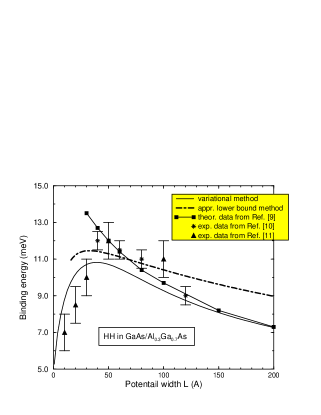
FIG. 3.: Comparison of results for the binding energy of an exciton in a rectangular quantum well as function of the well width.

A second class of confinement potentials is of parabolic type, that is

$$V_{i}(z)={m_{i}R_{\infty}^{2}{\lambda}^{2}_{i}\over 2{\hbar}^{2}}z_{i}^{2},$$ (15)

where $\lambda_{i}$ denotes the dimensionless confinement strength, $R_{\infty}$ is the Rydberg unit, which was extracted for reasons of convenience. To study the confinement-induced effects on the spectrum as accurately as possible, we disregarded any parameter mismatch. The quantity of interest is the diagonal element of the reduced density operator, namely

$$P_{\beta}({\bf{C}}):=<{\bf{C}}|tr_{Ph}e^{-{\beta}H}|{\bf{C}}>.$$ (16)

In this formula ${\bf{C}}$ is an abbreviation for an arbitrary (but fixed) set of the position coordinates of the particles involved. The right-hand side of Eq. (16) can be represented as a functional integral

$$P_{\beta}({\bf{C}})=Z_{Ph}\int\delta^{6}R\ e^{-S[{\bf{R}}]}.$$ (17)

In Eq. (17) $Z_{Ph}$ is the free-phonon partition function, and $S$ reads as follows:

$$S[{\bf{R}}] := \int_{0}^{\beta}d\tau\left(\sum_{n=1}^{2}\frac{m_{n}}{2}{\dot{\bf{R}}}_{n}^{2}(\tau)+U({\bf{R}}_{1}(\tau),{\bf{R}}_{2}(\tau))\right)$$ (19)

$$-\sum_{n,n^{\prime}=1}^{2}\sum_{{\bf{k}}}\frac{g_{{\bf{k}},n}g_{{\bf{k}},n^{\prime}}}{V}\int\limits_{0}^{\beta}\int\limits_{0}^{\beta}d\tau\,d\tau^{\prime}\,G(\tau-\tau^{\prime})\;e^{i{\bf{k}}[{\bf{R}}_{n}(\tau)-{\bf{R}}_{n^{\prime}}(\tau^{\prime})]}.$$

Within the functional integral (17), $\int\delta^{6}R....$ is to indicate integration over all real, $6$-dimensional paths ${\bf{R}}(\tau)$, which start and end at the point ${\bf{C}}$. The kernel function $G(\tau-{\tau}^{\prime})$ is defined as

$$G(\tau):={e^{\hbar\omega(\beta-|\tau|)}+e^{\hbar\omega|\tau|}\over 2[e^{\beta\hbar\omega}-1]}.$$ (20)

It is well known that functional integrals of type (17) with an action (19) cannot be evaluated in analytical form. Starting from the exact expression, we use variational procedures as in Feynman’s famous paper on polarons to find upper bounds on the ground-state energy. The necessary input is a trial action, which is accessible to a numerical treatment.

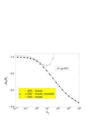
FIG. 4.: Binding energy of an exciton in a parabolic quantum well as function of the electron confinement strength $\lambda_{1}$. The comparison is made for different approaches described in Ref.[14]. The parameters $\sigma^{2}=m_{1}/m_{2}$ and $\chi=\lambda_{2}/\lambda_{1}$ are fixed as indicated.

The trial companions of the exact action (19) were combinations of oscillator trial actions for the center-of-mass and the $z$-coordinate and three-dimensional (two-dimensional) Coulomb potentials for the three-dimensional (two-dimensional in-plane) relative coordinates. The corresponding results (see Ref. [14]) can be found in the following figures and are denoted as quasi three-dimensional (Q3D) and quasi two-dimensional (Q2D or Q2Dalt) ansatz. In Fig. 4 we neglect any phonon influence to demonstrate the smooth interpolation of the limiting values $1R_{\infty}$ and $4R_{\infty}$ of the binding energy (actually we plotted there the ground-state energy with the continuum edge being subtracted, that is, the quantity $-E_{B}$). Fig. 5 shows results for the general case; we present data for the ground-state energy as well as the continuum edge, which is the reference for the binding energy and has to be calculated separately.

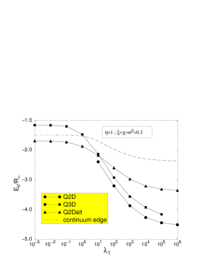
FIG. 5.: Ground-state energy of an exciton-phonon system in a parabolic quantum well as function of the confinement electron strength $\lambda_{1}$. The remaining parameters $\eta=\sqrt{R_{\infty}/\hbar\omega}$ and $\xi=1-\varepsilon_{\infty}/\varepsilon_{0}$ are fixed as indicated. In addition, an upper bound for the energy of the continuum edge is shown.

The results reported have been obtained in collaboration with M. Dzero and J. Wüsthoff; we gratefully thank both of them. We are indebted to J. T. Devreese, V. Gladilin, H. Leschke, V. M. Fomin, F. M. Peeters, and E. P. Pokatilov for useful discussions and remarks. The support of Deutsche Forschungsgemeinschaft and the Germany-JINR Heisenberg-Landau program is acknowledged.

REFERENCES

- [1] E-mail address: gerlach@fkt.physik.uni-dortmund.de
- [2] E-mail address: smond@thsun1.jinr.dubna.su
- [3] M. Kumagai, T. Takagahara, Phys. Rev. B 40, 12359 (1989).
- [4] G. Hai, F. M. Peeters, and J. T. Devreese. Phys. Rev. B 48, 4666 (1993).
- [5] J. J. Shi, X. Q. Zhu et al. Phys. Rev. B 55, 4670 (1997).
- [6] H. Kleinert and I. Mustapić. J. Math. Phys. 33, 643 (1992).
- [7] W. Fischer, H. Leschke, and P. Müller. In: Path Integrals from meV to MeV: Tutzing ’92, ed. H. Grabert, A. Inomata, L. S. Schulman, U. Weiss (World Scientific, Singapore, 1993), p. 259; Ann. Phys. 227, 206 (1993).
- [8] S. Adachi. J. Appl. Phys. 58, R1 (1985).
- [9] M. Smondyrev, B. Gerlach, and M. Dzero, 1999 (unpublished).
- [10] B. Gerlach, J. Wüsthoff, M. Dzero, and M. Smondyrev, Phys. Rev. B 58, 10568 (1998).
- [11] L. C. Andreani, A. Pasquarello, Phys. Rev. B 42, 8928 (1990).
- [12] M. Gurioli, J. Martinez-Pastor et al. Phys. Rev. B 47, 15755 (1993).
- [13] V. Voliotis, G. Grousson, P. Lavallard, and R. Planel, Phys. Rev. B 52, 10725 (1995).
- [14] B. Gerlach, J. Wüsthoff, and M. Smondyrev, Phys. Rev. B 60, 16569 (1999).