Cryptoferromagnetic state in superconductor-ferromagnet multilayers

Abstract

We study a possibility of a non-homogeneous magnetic order (cryptoferromagnetic state) in heterostructures consisting of a bulk superconductor and a ferromagnetic thin layer that can be due to the influence of the superconductor. The exchange field in the ferromagnet may be strong and exceed the inverse mean free time. A new approach based on solving the Eilenberger equations in the ferromagnet and the Usadel equations in the superconductor is developed. We derive a phase diagram between the cryptoferromagnetic and ferromagnetic states and discuss the possibility of an experimental observation of the CF state in different materials.

PACS: 74.80.Dm,74.50.+r, 75.10.-b

In the last years, the interest in experiments on superconducting-ferromagnet ($S/F$) hybrid structures has grown rapidly. Such structures show the coexistence of these two antagonistic orderings but their mutual influence is still a controversial point [1, 2, 3, 4, 5, 6]. In these experiments, the multilayers contained strong ferromagnets like $Fe$ or $Gd$ with the Curie temperature up to $1000K$ and superconductors with transition temperatures not exceeding $10K$, like $Nb$ or $V$.

Naturally, in most theoretical works only the influence of the ferromagnet on the superconductivity of $S/F$ systems was considered [7, 8, 9]. One may argue that a modification of the magnetic ordering would need energies of the order of the Curie, which is much larger than the superconducting transition temperature $T_{c}$. Therefore, any change of the ferromagnetic order would be less energetically favorable than the destruction of the superconductivity in the vicinity of the ferromagnet.

This simple argument was questioned in a recent experimental work [10], where $Nb/Fe$ bilayers were studied using different experimental techniques. Direct measurements using the ferromagnetic resonance showed that in several samples with thin ferromagnetic layers $(10-15$Å$)$ the average magnetic moment started to decay at the superconducting transition temperature $T_{c}$. The measurements were possible only in a limited range of the temperatures below $T_{c}$ and the decrease of the magnetic moment in this interval reached $10\%$ without any sign of a saturation. As a possible explanation of the effect, it was assumed in Ref. [10] that the superconductivity affected the magnetic order causing a domain-like structure.

A possibility of a domain-like magnetic structure in presence of superconductivity has been first suggested by Anderson and Suhl long ago [11]. They argued that a weak ferromagnetism of localized electrons should not destroy the superconductivity in the conduction band. Instead, it may become more favorable energetically to build a domain structure called cryptoferromagnetic state [11]. Later this state was investigated both theoretically and experimentally in detail (for review see, e.g.[12]).

In this paper, we investigate theoretically the possibility of a cryptoferromagnetic-like (CF) state in $S/F$ bilayers with parameters corresponding to the structures used in the experiments [1, 2, 3, 4, 5, 6, 10]. Such a study is very important because it may allow to clarify the question about the cryptoferromagnetic state in the experiment [10] and to make predictions for other $S/F$ multilayers. From the theoretical point of view, large magnetic energies involved make the problem quite non-trivial and demand development of new approaches.

To the best of our knowledge the possibility of a non-homogeneous magnetic order in multilayers was considered only in Ref. [13]. However, although the authors of Ref. [13] came to the conclusion that the domain-like structure due to the interaction with the superconductor was possible, the results obtained can hardly be used for quantitative estimates. For example, they assumed that the period of the structure $b$ had to be not only much smaller than the size of the Cooper pair $\bar{\xi}$, but also than $\bar{\xi}\sqrt{T_{c}/h}$, where $h$ is the energy of interaction of conduction electrons (CEs) with the localized magnetic moments (LMs). In addition, a very rough boundary condition at the $S/F$ boundary was used.

In contrast, we present here a microscopic derivation of the phase diagram valid for realistic parameters of the problem involved. We will show that the phase transition between the CF and ferromagnetic (F) phases is continuous and the period of the structure $b$ goes to infinity at the critical point. The only restrictions we use are

$$d\ll\xi_{F}=v_{0}/h,\qquad T_{c}\ll h\ll\epsilon_{0}$$ (1)

where $d$ is the thickness of the ferromagnetic layer, $v_{0}$ and $\varepsilon_{0}$ are the Fermi-velocity and Fermi-energy.

Even in the such strong ferromagnet as iron, $\xi_{F}$ is of the order $10$Å. For weaker ferromagnets like $Gd$, $\xi_{F\text{ \ }}$is considerably larger and the inequalities (1) can be fulfilled rather easily.

We assume that the superconductor occupies the half-space $x>0$ while the ferromagnetic film occupies the region $-d<x<0$ and write the Hamiltonian as

$$H\!\!\!=\!H_{BCS}+\!\!\gamma\!\!\int d{\bf r}\Psi_{\alpha}^{+}({\bf r})\left[{\bf h}({\bf r}){\bf\sigma}\right]_{\alpha\beta}\Psi_{\beta}({\bf r})+H_{M}$$ (2)

where $H_{BCS}$ is the usual BCS Hamiltonian (in the presence of non-magnetic impurities) describing the superconducting state in the $S$ layer, $\gamma$ is a constant which will be put to 1 at the end. The second term in Eq. (2) stands for the interaction between the LMs of the ferromagnet and the CEs, where $\!{\bf h}$ is the exchange field and ${\bf\sigma}$ is the vector containing the Pauli matrices as components. We neglect the influence of the LMs on the orbital motion of the CEs since the exchange interaction is the dominant Cooper pair breaking mechanism [12] for the problem involved. The term $H_{M}$ describes the interaction between the LM in the ferromagnet.

Our aim is to obtain an expression for the free energy of the system for different magnetic structures in the F layer. To determine the contribution of an inhomogeneous alignment of magnetic spins to the total energy we use the limit of a continuous material and replace the spins by classical vectors. We assume that the anisotropy energy of the ferromagnet is smaller than the exchange energy and hence there is no easy axis of magnetization. This can definitely be a good approximation for iron with a cubic lattice used in the work [10]. The energy $H_{M}$ of a non-homogeneous structure can be written in the continuum limit as

$$H_{M}=\int J\left[\left({\bf\nabla}S_{x}\right)^{2}+\left({\bf\nabla}S_{y}\right)^{2}+\left({\bf\nabla}S_{z}\right)^{2}\right]dV,$$ (3)

where the magnetic stiffness $J$ characterizes the strength of the coupling between LMs in the F layer and $S_{i}$’s are the components of a unit vector. Writing ${\bf S}=\left(0,-\sin\Theta,\cos\Theta\right)$ and minimizing the energy $H_{M}$ we obtain the equation $\Delta\Theta=0$. We consider only the solutions of this equation that are of interest for us:

$$a)\text{ }\Theta=0,\text{ \ \ \ \ \ \ }b)\text{\ }\Theta=Qy$$ (4)

The solution a) in Eq. (4) corresponds to the F state, whereas the solution b) describes a CF state with a homogeneously rotating magnetic moment. The wave vector of this rotation is denoted by $Q$. The magnetization is chosen to be parallel to the FS interface, i.e. to the $yz-$plane. This allows to neglect Meissner currents in the superconductor. With all this assumptions the magnetic energy $\Omega_{M}$ (per unit surface area) is given by

$$\Omega_{M}=JdQ^{2}$$ (5)

The corresponding energy of the F state equals zero.

The superconducting part of the energy can be calculated deriving from Eq. (2) proper Eilenberger equations [14] for the superconductor and the ferromagnet, solving these equations and then matching the solutions. In practice, this is difficult and we simplify the problem considering the “dirty limit” $l\ll\xi_{0}$, where $l$ is the mean free path and $\xi_{0}=v/T_{c}$ is the coherence length of the superconductor in the clean limit, which allows to use the more simple Usadel equations [15]. If we assume that $|\tau|\ll 1$, $\tau=\left(T-T_{c}\right)/T_{c}$, the Usadel equations together with the self-consistency equation can be further reduced to the Ginzburg-Landau (GL) equation[16, 17, 18]. However, the latter equation can be used only sufficiently far from the $S/F$ boundary at distances exceeding $\bar{\xi}\sim\sqrt{\xi_{0}l}$. At the distances of the order of $\bar{\xi}$ one should write again the Usadel equations but in the limit $|\tau|\ll 1$ they can be linearized. This is a conventional scheme of calculation for interfaces between superconductors and normal metals or ferromagnets.

Writing the Usadel equations in the ferromagnet may not be a good approximation because the exchange energy $h$ in realistic cases is not necessarily smaller than $1/\tau_{tr}$, where $\tau_{tr}$ the mean free time, and so one should write in this region the Eilenberger equations. At the end one should match the solutions of all the equations.

Now we start the calculations following this program. The loss of the superconducting energy due to the suppression of the superconductivity in the $S$-layer can be found from the solution of the GL equation for the order parameter $\Delta({\bf r})$. At distances $x\gg\bar{\xi}$, the proper solution is [16, 17, 18]

$$\Delta(x)=\Delta(T)\tanh\left(\frac{x}{\sqrt{2}\xi(T)}+C\right),$$ (6)

where $\Delta(T)=\sqrt{\frac{8\pi^{2}}{7\zeta(3)}|\tau|}T_{c}\equiv\Delta_{0}\tau^{1/2}$ is the value of the order parameter in the bulk superconductor, $\xi(T)=\sqrt{\frac{\pi D}{8T_{c}}}|\tau|^{-1/2}$ is the characteristic scale of the spacial variation of $\Delta\left({\bf r}\right)$, $D$ is the diffusion coefficient in the superconductor, and $C$ is a constant. Substituting $\Delta\left(x\right)$, Eq. (6), into the GL free energy functional one can evaluate the loss of the superconducting energy at the $F/S$ interface per unit surface area as function of $C$[17]

$$\Omega_{S}=\frac{\sqrt{\pi}}{6\sqrt{2}}|\tau|^{3/2}\left(2+K\right)(1-K)^{2}$$ (7)

where $K=\tanh C$. The influence of the ferromagnet on the superconductivity is determined by the parameter $K$ that will be found by minimizing the total energy.

The contribution $\Omega_{M/S}$ of the second term in (2) to the total energy has still to be determined. First, we write the Eilenberger equation for the magnetic moment ${\bf h}\left({\bf r}\right)$ depending on coordinates. Introducing the quasiclassical matrix Green function $\check{g}_{\omega}({\bf r},{\bf p}_{0})$

$\displaystyle\check{g}=\left(\begin{array}[]{cc}\hat{g}&-\hat{f}\\ \hat{f}^{+}&-\hat{g}^{+}\end{array}\right)$

one derives in the standard way the Eilenberger equation in the spin$\otimes$particle-hole space

$$\left[\left\{\omega\check{\tau}_{3}-i\check{\Delta}+i\gamma\check{V}+i\check{\Sigma}{\it{}_{imp}}\right\},\check{g}\right]+{\bf v}_{0}\nabla_{{\bf r}}\check{g}=0\,.$$ (8)

where ${\bf p}_{0}$ and ${\bf v}_{0}$ are the momentum and velocity at the Fermi-surface.

In Eq. (8), $\check{\tau}_{i}$, $i=1,2,3$, are Pauli matrices in the particle-hole space, $\check{\Delta}\!\!=\!\!\check{\tau}_{1}\otimes i\sigma_{y}\Delta({\bf r})$, $\check{V}={\rm Re}\left({\bf h}({\bf r}){\bf\sigma}\right)\otimes\check{1}+{\rm Im}\left({\bf h}({\bf r}){\bf\sigma}\right)\otimes\check{\tau}_{3}$, and $\Delta$ should be determined self-consistently

$$\Delta({\bf r})=-\frac{i}{2}\pi\nu\lambda_{0}T\sum_{n}<f_{12}({\bf r},{\bf p}_{0},\omega_{n})>_{0}\,,$$ (9)

where $\left\langle...\right\rangle_{0}$ denotes averaging over the Fermi velocity and $\lambda_{0}$ is the constant of the electron-electron interaction, $\nu$ is the density of states. We assume for simplicity that $\lambda_{0}=0$ and hence $\Delta=0$ in the ferromagnet. At the same time, $h=0$ in the superconductor. The term $i\check{\Sigma}_{{\it imp}}$ describes scattering by impurities. For a short range interaction, $\check{\Sigma}_{{\it imp}}=-\frac{i}{2\tau}\left\langle\check{g}\right\rangle_{0}$. Eq. (8) is complemented by the normalization condition $\check{g}^{2}=\check{1}$. Once we know $\hat{g}$, we can determine $\Omega_{M/S}$ using the expression [16]:

$$\Omega_{M/S}=-i\pi T\nu_{0}\sum_{\omega}\int_{0}^{1}d\gamma\int d^{3}{\bf r}({\bf h\sigma})_{\alpha\beta}\left\langle g_{\beta\alpha}\right\rangle_{0}\,$$ (10)

Near $T_{c}$, the anomalous functions $\hat{f}$ and $\hat{f}^{+}$ are small and $\hat{g}\approx sgn\left(\omega\right)$. Then, in the limit $T_{c}\ll h$ the off-diagonal component (1,2) in particle-hole space of the equation (8) in the region $-d<x<0$ is

$${\bf v}_{0}\nabla\hat{f}\!\! = \!\!-i\hat{V}\hat{f}^{(F)}+i\hat{f}^{(F)}\hat{V}^{\ast}\!\!-\frac{sgn\left(\omega\right)}{\tau}(\hat{f}^{(F)}-<\!\hat{f}^{(F)}\!>)$$ (11)

$$\hat{V} = h(x)\sigma_{z}\exp(iQy\sigma_{x})$$ (12)

$h$ is the strength of the exchange field in the $F$-layer.

Assuming that $d\ll v_{0}/h$ we can relate the values of the function $\hat{f}^{(F)}({\bf v}_{{\bf 0}},{\bf r})$ at the interface, i.e. at $x=0^{-}$ to the values at the boundary to the vacuum at $x=-d$ using the Taylor expansion:

$$\hat{f}^{(F)}({\bf v}_{0},{{\bf r}_{0}}-{\bf r}_{{\bf d}})\approx\hat{f}^{(F)}({\bf v}_{0},{{\bf r}_{0}})-d\partial_{x}\hat{f}^{(F)}({\bf v}_{0},{\bf r}_{0})\,,$$ (13)

where ${{\bf r}_{0}}=(0,y,z)$ and ${\bf r}_{{\bf d}}=(-d,y,z)$ . Applying general boundary conditions [19] to the problem involved we conclude that for a perfectly transparent interface the function $\hat{f}$ is continuous at the interface. At the boundary with the vacuum ($x=-d$) the function $\hat{f}$ satisfies

$$\hat{f}^{(F)}(v_{x},{\bf r}_{0}-{\bf r}_{{\bf d}})=\hat{f}^{(F)}(-v_{x},{\bf r}_{0}-{\bf r}_{{\bf d}})$$ (14)

Using Eqs. (11, 13, 14) and the continuity of $\hat{f}$ at ${\bf r}={\bf r}_{0}$ the problem is reduced to the solving of the Usadel equation in the superconductor with the following effective boundary condition at the interface

$$\eta D(\partial_{x}+d\partial_{y}^{2})\hat{f}_{0}({\bf r}_{0})+isgn\left(\omega\right)\left(-\hat{V}\hat{f}_{0}+\hat{f}_{0}\hat{V}^{\ast}\right)_{\!\!{\bf r}_{0}}\!\!\!\!=\!\!0$$ (15)

where $\eta=v_{0}^{F}/v_{0}^{S}$ and $\hat{f}_{0}$ is the zero harmonics of the function $\hat{f}$ in the superconductor. When deriving Eq. (15) we used the fact that the Usadel equation is applicable in the $S$- layer at distances down to the mean free path $l$ and extrapolated its solution to the interface. Only first two spherical harmonics $\hat{f}^{(s)}\approx\hat{f}_{0}+{\bf v}_{{\bf 0}}\hat{{\bf f}}_{1}$ were kept in the derivation.

The linearized Usadel equation for the superconductor can be written in the standard form

$$D\nabla^{2}\hat{f}_{0}-2|\omega|\hat{f}_{0}-2\Delta(x)\sigma_{y}=0$$ (16)

The general solution of Eq. (16) with the boundary condition, Eq. (15), and $\hat{V}$ from Eq. (11) can be written as

$$\hat{f}_{0}({\bf r},\omega)=\alpha_{\omega}(x)\sigma_{x}e^{-i\sigma_{x}Qy}+\beta_{\omega}(x)i\sigma_{y\,,}$$ (17)

where $\alpha_{\omega}(x)=C_{\omega}\exp\left(-\sqrt{Q^{2}+\frac{2|\omega|}{D}}x\right)$ and $\beta_{\omega}(x)=-i\frac{\Delta(x)}{|\omega|}+B_{\omega}\exp\left(-\sqrt{\frac{2|\omega|}{D}}x\right)$. Eq. (17) is applicable at distances much smaller than $\xi\left(T\right)$, where the solution for $\Delta$ can be approximated by a linear function. One can check using the self-consistency Eq. (9) that the relative correction to $\Delta$ coming from the exponentially decaying part of Eq. (17), is of the order $\left(\ln\frac{\omega_{D}}{T_{c}}\right)^{-1}$, where $\omega_{D}$ is the Debye frequency, and we neglected it. The coefficients $C_{\omega}$ and $B_{\omega}$ can be now determined from Eq. (15). Using the condition $\check{g}^{2}=1$ and Eq. (10) we can find the energy $\Omega_{M/S}$. Introducing the dimensionless parameters:

$$a^{2}\equiv\frac{2h^{2}d^{2}}{DT_{c}\eta^{2}}\text{, \ }q^{2}\equiv\frac{DQ^{2}}{2T_{c}}\text{, \ \ }\widetilde{\Omega}\equiv\frac{\Omega}{\nu_{F}\Delta_{0}^{2}}\sqrt{\frac{2T_{c}}{D}}$$ (18)

and using Eq. (6) one obtains

$$\widetilde{\Omega}_{M/S} = \frac{\pi}{2}F_{3/2,1}K^{2}|\tau|+\sqrt{2}F_{2,1}K\left(1-K^{2}\right)|\tau|^{3/2}$$ (20)

$$+\pi^{-1}F_{5/2,1}\left(1-K^{2}\right)^{2}|\tau|^{2},$$

$$F_{m,l} = \eta\frac{4a^{2}}{\pi^{3/2-m}}\sum_{n>0}\alpha_{n}^{-m}\left[\sqrt{\alpha_{n}\left(\alpha_{n}+q^{2}\right)}+a^{2}\right]^{-l}$$ (21)

where $\alpha_{n}=\pi(2n+1)$ and $\nu_{F}$ is the density of states in the ferromagnet.The total energy is given by $\widetilde{\Omega}=\widetilde{\Omega}_{M}+\widetilde{\Omega}_{S}+\widetilde{\Omega}_{M/S}$, Eqs. (5, 7, 20) and is a functions of two parameters, $K$ and $q$, that should be determined from the conditions $\partial\widetilde{\Omega}/\partial K=\partial\widetilde{\Omega}/\partial q=0$. The parameter $q$ is in fact the order parameter for the CF state. Close to the CF-F transition this parameter is small and one can expand the energy $\widetilde{\Omega}_{M/S}$, Eq. (20), in $q^{2}$. As concerns the value $K_{0}$ at the minimum, it can be found near the transition minimizing $\widetilde{\Omega}_{M/S}$ at $q=0$. As a result, the first terms of the expansion of the energy $\widetilde{\Omega}$ in $q^{2}$ near the CF-F transition can be written as

$$\scriptstyle\begin{array}[]{l}\widetilde{\Omega}\approx\widetilde{\Omega}_{s}(K_{0})+\widetilde{\Omega}_{M/S}(K_{0},q=0)-\\ -\frac{q^{2}}{2}\left[\frac{\pi}{2}F_{3/2,2}K_{0}^{2}|\tau|+\sqrt{2}F_{2,2}K_{0}(1-K_{0}^{2})|\tau|^{\frac{3}{2}}+\right.\\ \left.+\pi^{-1}F_{5/2,2}\left(1-K_{0}^{2}\right)^{2}|\tau|^{2}-2\lambda\right]_{q=0}\end{array}$$ (22)

One can check that the term proportional to $q^{4}$ is positive, which means that the CF-F transition is of the second order. This is in contrast to the conclusion of Ref. [13]. The parameter $\lambda$ in Eq. (22) is

$$\lambda\equiv\frac{Jd}{\nu\sqrt{2T_{c}D^{3}}}\frac{7\zeta(3)}{2\pi^{2}}$$ (23)

According to the Landau theory of phase transitions the transition from the F state ($q=0$) to the CF state ($q\neq 0$) should occur when the coefficient in the second-order term turns to zero. The phase diagram for the variables $h$ and $J$, Eqs. (18, 23), is represented in Fig.1. The curves are plotted for different values of $|\tau|$. The function $\widetilde{\Omega}(q)$ has only one minimum at $q_{0}$ continuously going to zero as the system approaches the transition point.This demonstrates that the transition is of second order. Not close to the transition point $Q\sim\bar{\xi}^{-1}$.

The stiffness $J$ for materials like $Fe$ and $Ni$ is $\approx 60K/$Å. Using the data for Nb $T_{c}\!=\!10$Å, $v_{F}\!=\!1,37.10^{8}$cm/s, setting $l\!=\!100$Å, $d\!=\!10$Å, and $h\!=\!10^{4}$K, which is proper for iron, and assuming that the Fermi velocities and energies of the ferromagnet and superconductor are close to each other we obtain $a\approx 25$ and $\lambda\sim 6.10^{-3}$. It is clear from Fig.1 that the CF state is hardly possible in the $Fe/Nb$ structure studied in [10].

How can one explain the decay of the average magnetic moment below $T_{c}$ observed in that work? This can be understood if one assumes that there were “islands” in the magnetic layers with smaller values of $J$ and/or $h$. A reduction of these parameters in the multilayers $Fe/Nb$ is not unrealistic because proximity to $Nb$ leads to formation of non-magnetic “dead” layers [4], and can affect the parameters of the ferromagnetic layers, too. If the CF state were realized only on the islands, the average magnetic moment would be reduced but remain finite, which would correlate with the experiment [10]. One can also imagine islands very weakly connected to the rest of the layer, which would lead to smaller energies of a non-homogeneous state.

Another possibility to observe the CF state would be to use multilayers with a weaker ferromagnet. A good candidate for this purpose might be $Gd/Nb$. The exchange energy $h$ in $Gd$ is $h\approx 10^{3}K$ and the Curie temperature and, hence, the stiffness $J$ is $3$ times smaller than in $Fe$. So, one can expect $a\approx 2.5$ and $\lambda\approx 2.10^{-3}$. Using Fig.1 we see that the CF phase is possible for these parameters. One can also considerably reduce the exchange energy $h$ in $V_{1-x}Fe_{x}/V$ multilayers [6] varying the alloy composition. Hopefully, the measurements that would allow to check the existence of the CF phase in these multilayers will be performed in the nearest future.

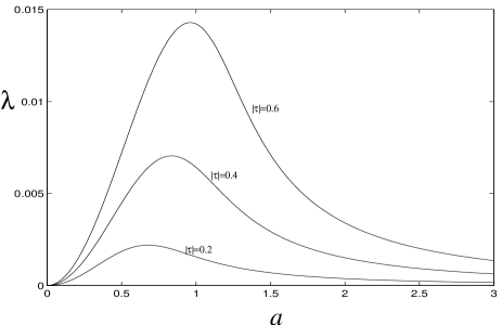
FIG. 1.: Phase diagrams ($\lambda,a$). The area above (below) the curves corresponds to the F (CF) state

In conclusion, we studied a possibility of the CF state in ($S/F$) multilayers. We derived a phase diagram that allows to make definite predictions for real materials.

We are grateful to I.A. Garifullin for numerous discussion of experiments and to D. Taras-Semchuck and F.W.J. Hekking for helpful discussions. F.S.B. and K.B.E. thank SFB 491 Magnetische Heterostrukturen for a support. The work of A.I.L. was supported by the NSF grant DMR-9812340 and the A.v. Humboldt Foundation.

REFERENCES

- [1] P.Koorevaar et al., Phys. Rev. B 49, 441 (1994)
- [2] C. Strunk et al., Phys. Rev. B 49, 4053 (1994)
- [3] J.S. Jiang et al., Phys.Rev. Lett. 74, 314 (1995)
- [4] Th. Mühge et al., Phys. Rev. Lett. 77, 1857 (1996)
- [5] G. Verbanck et al., Phys. Rev. B 57, 6029 (1998)
- [6] J. Aarts et al., Phys. Rev. B 56, 2779 (1997)
- [7] Z. Radovic et al., Phys. Rev. B 38, 2388 (1988); Z. Radovic et al., Phys. Rev. B44, 759 (1991); A. I. Buzdin et al., Physica (Amsterdam), 185C, 2025 (1991)
- [8] O. Sipr et al., J.Phys. Cond.Matt. 7, 5239 (1995)
- [9] C.A.R. Sa de Melo, Phys. Rev. Lett. 79, 1933 (1997)
- [10] Th. Mühge et al., Physica C, 296, 325 (1998)
- [11] P.W.Anderson and H. Suhl, Phys. Rev. 116, 898 (1959)
- [12] L.N.Bulaevskiiet al., Advances in Physics 34, 175 (1985)
- [13] A.I.Buzdin and L.N. Bulaevskii, Sov. Phys. JETP 67, 576 (1988)
- [14] G. Eilenberger, Z. Phys. 214,195 (1968); A.I. Larkin and Yu.N. Ovchinnikov, Sov. Phys. JETP 28,1200 (1969)
- [15] K.D.Usadel, Phys. Rev. Lett. 25, 507 (1970)
- [16] A. Abrikosov, L. Gorkov and I. Dzyaloshinski, Methods of Quantum Field Theory in Statistical Physics (Dover Publications, N.Y.,1963)
- [17] P.G. de Gennes, Superconductivity of Metals and Alloys (Benjamin, 1966)
- [18] A.A.Abrikosov, Fundamentals of the Theory of Metals (North-Holland, Amsterdam,1988)
- [19] A.V.Zaitsev, Sov. Phys. JETP 59,1015 (1985)