Thermodynamic properties
of the periodic nonuniform spin-$\frac{1}{2}$ isotropic $XY$ chains
in a transverse field

Abstract

Using the Jordan-Wigner transformation and the continued-fraction method we calculate exactly the density of states and thermodynamic quantities of the periodic nonuniform spin-$\frac{1}{2}$ isotropic $XY$ chain in a transverse field. We discuss in detail the changes in the behaviour of the thermodynamic quantities caused by regular nonuniformity. The exact consideration of thermodynamics is extended including a random Lorentzian transverse field. The presented results are used to study the Peierls instability in a quantum spin chain. In particular, we examine the influence of a non-random/random field on the spin-Peierls instability with respect to dimerization.

PACS numbers: 75.10.-b

Keywords: Spin-$\frac{1}{2}$ $XY$ chain; Periodic nonuniformity; Diagonal Lorentzian disorder; Density of states; Thermodynamics; Spin-Peierls dimerization

Postal addresses:

Dr. Oleg Derzhko (corresponding author)
Oles’ Zaburannyi
Institute for Condensed Matter Physics
1 Svientsitskii St., L’viv-11, 290011, Ukraine
Tel: (0322) 42 74 39
Fax: (0322) 76 19 78
E-mail: derzhko@icmp.lviv.ua

Prof. Johannes Richter
Institut für Theoretische Physik, Universität Magdeburg
P.O. Box 4120, D-39016 Magdeburg, Germany
Tel: (0049) 391 671 8841
Fax: (0049) 391 671 1217
E-mail: Johannes.Richter@Physik.Uni-Magdeburg.DE

1 Introduction

The study of regularly nonuniform spin models is an attracting problem of statistical mechanics. Besides of its general academic importance the development of magnetic materials in recent years makes the study of nonuniform spin models particularly interesting for experimental application. In order to achieve a progress in understanding the generic features generated by periodic nonuniformity it is desirable to examine simple models that may be investigated without making any approximation. Among possible candidates of such systems one can mention the spin-$\frac{1}{2}$ $XY$ model in one dimension. The uniform one-dimensional spin-$\frac{1}{2}$ $XY$ model in a transverse field was introduced by Lieb, Schultz and Mattis.¹ These authors noticed that a lot of statistical mechanics calculations for such a spin model can be performed exactly since it can be rewritten as a model of noninteracting spinless fermions by means of the Jordan-Wigner transformation. The nonuniform version of the transverse spin-$\frac{1}{2}$ $XY$ chain also can be mapped onto a chain of free spinless fermions, however, with an on-site energy and hopping integrals that vary from site to site. Especially attractive is the case of isotropic spin coupling with regularly alternating exchange integrals and transverse fields since after fermionization one faces a model for which a lot of work has been done. One should mention here the results for the tight-binding Hamiltonian of periodically modulated chains^2,3 and the spinless Falicov-Kimball chain.^4,5

One of the goals of the present paper is to give a magnetic interpretation of those results derived for the one-dimensional tight-binding spinless fermions. Exploiting the continued-fraction approach developed in the mentioned papers^2-5 we shall be able to calculate exactly the one-fermion Green functions and therefore to obtain the thermodynamic quantities for the periodic nonuniform spin-$\frac{1}{2}$ isotropic $XY$ chain in a transverse field. We shall treat few examples of the periodic nonuniform spin-$\frac{1}{2}$ isotropic $XY$ chain in a transverse field in order to reveal the changes in the thermodynamic properties induced by periodic nonuniformity. The model of the considered regularly nonuniform magnetic chain allows even a natural extension to include additional disorder remaining the model exactly solvable. Namely, one can assume the transverse fields to be random independent Lorentzian variables with regularly alternating mean values and widths of distribution. To derive exactly the random-averaged density of states for such a model one should at first average a set of equations for the Green functions using contour integrals.^6-11 As a result one comes to a set of equations similar to that for the periodic nonuniform non-random case.

It should be noted that the periodic nonuniform spin-$\frac{1}{2}$ isotropic $XY$ chain was considered in several papers^12-25 dealing mainly with the adiabatic treatment of the spin-Peierls instability. However, those papers were focussed mostly on the influence of the structural degrees of freedom upon the magnetic ones, rather than on the exhaustive analysis of the properties of a magnetic chain with regularly alternating exchange couplings. Another closely related study concerns the spin-$\frac{1}{2}$ isotropic $XY$ model on a one-dimensional superlattice²⁶. The treatment reported in Ref. 26, however, was restricted to the magnon spectrum. A related study of the spin-$\frac{1}{2}$ isotropic $XY$ chain in a transverse field with two kinds of coupling constant aimed on examining the condition for appearance of an energy gap was reported in Ref. 27. Finally, let us note that the periodic nonuniform chain can be viewed as the uniform chain with a crystalline unit cell containing several sites of the initial lattice (as a matter of fact such a point of view was adopted, for example, in Refs. 12, 13) and thus the standard methods elaborated for such complex crystals may be exploited. However, we prefer to treat periodically nonuniform chains since from such a viewpoint an elegant continued-fraction approach immediately arises that seems to be a natural and convenient language for describing such compounds.

The present paper is a more extensive version of the results briefly reported in Refs. 28, 29 containing more details on the calculation and more applications. We show that the presented below method based on continued-fraction representation for the one-fermion diagonal Green functions immediately reproduces the results for the spin-$\frac{1}{2}$ transverse isotropic $XY$ chains having periods 2 and 3 and in contrast to other approaches easily yields the results for larger periods (e.g., 4 and 12). It should be stressed that the elaborated approach is a systematic method that permits to consider in the same fashion the regularly nonuniform chains with randomness that cannot be done within the frames of the approaches exploited in Refs. 12-27. We present a comprehensive study of the thermodynamic properties (density of states, gap in the energy spectrum, entropy, specific heat, magnetization, susceptibility) of regularly alternating chains having periods 2, 3, 4, and 12 discussing in detail the dependences of the energy gap and the low-temperature transverse magnetization on the transverse field and comparing the latter dependence with the corresponding one for the classical spin chain. We underline a possibility of a nonzero transverse magnetization at the zero average transverse field in the periodic nonuniform chain owing to a regular nonuniformity. This material constitutes Section 2. In Section 3 we demonstrate the influence of a diagonal disorder on the effects caused by periodic nonuniformity assuming the transverse fields to be independent random Lorentzian variables. For simplicity we restrict ourselves by the case of a chain having period 2. The results obtained for the spin-$\frac{1}{2}$ transverse isotropic $XY$ chains with period 2 are applied for an analysis of the spin-Peierls instability in the adiabatic limit with respect to dimerization in the presence of a non-random/random (Lorentzian) transverse field (Section 4). We find how the (random) transverse field influences the dependence of the (averaged) total energy on the dimerization parameter tracing a suppression of dimerization by the non-random (random) field.

2 Periodic nonuniform spin-$\frac{1}{2}$ isotropic $XY$ chain in a transverse field

Let us consider a cyclic nonuniform isotropic $XY$ chain of $N$ (eventually $N\to\infty$) spins $s=\frac{1}{2}$ in a transverse field. The Hamiltonian of the system reads

$$H=\sum_{n=1}^{N}\Omega_{n}s_{n}^{z}+2\sum_{n=1}^{N}I_{n}\left(s^{x}_{n}s^{x}_{n+1}+s^{y}_{n}s^{y}_{n+1}\right)$$

$$=\sum_{n=1}^{N}\Omega_{n}\left(s_{n}^{+}s_{n}^{-}-\frac{1}{2}\right)+\sum_{n=1}^{N}I_{n}\left(s^{+}_{n}s^{-}_{n+1}+s^{-}_{n}s^{+}_{n+1}\right),\;\;\;s^{\alpha}_{n+N}=s^{\alpha}_{n}.$$ (1)

Here $\Omega_{n}$ is the transverse field at site $n$ and $2I_{n}$ is the exchange coupling between the sites $n$ and $n+1$. Let us note that $s^{z}=\sum_{n=1}^{N}s_{n}^{z}$ commutes with the Hamiltonian $H$ (1) and hence the eigenfunctions of $H$ can be classified according to eigenvalues of $s^{z}$. Moreover, at $\Omega_{n}=0$ the ground state of $H$ corresponds to $s^{z}=0$. After making use of the Jordan-Wigner transformation one comes to a cyclic chain of spinless fermions governed by the Hamiltonian

$$H=\sum_{n=1}^{N}\Omega_{n}\left(c_{n}^{+}c_{n}-\frac{1}{2}\right)+\sum_{n=1}^{N}I_{n}\left(c^{+}_{n}c_{n+1}-c_{n}c^{+}_{n+1}\right).$$ (2)

The so-called boundary term is not essential for calculation of thermodynamic functions³⁰ and has been omitted. We shall discuss the most general case, i.e. assuming that both transverse fields and exchange couplings vary from site to site. Note, that in the particular case when the transverse field is uniform one recognizes in Eq. (2) the Hamiltonian of the system considered in Ref. 2. In addition, in another limiting case after substitution $\Omega_{n}\rightarrow Uw_{n},$ $I_{n}\rightarrow-t$ Eq. (2) transforms into the Hamiltonian of a one-dimensional spinless Falicov-Kimball model in the notations used in Refs. 4, 5.

Let us introduce the temperature double-time Green functions $G_{nm}^{\mp}(t)=\mp{\mbox{i}}\theta(\pm t)\langle\left\{c_{n}(t),c_{m}^{+}(0)\right\}\rangle,$ $G_{nm}^{\mp}(t)=\left(1/2\pi\right)\int_{-\infty}^{\infty}{\mbox{d}}\omega\exp\left(-{\mbox{i}}\omega t\right)G_{nm}^{\mp}(\omega\pm{\mbox{i}}\epsilon),$ $\epsilon\rightarrow+0,$ where the angular brackets denote the thermodynamic average. Consider further the set of equations of motion for $G_{nm}^{\mp}\equiv G_{nm}^{\mp}(\omega\pm{\mbox{i}}\epsilon)$

$$\left(\omega\pm{\mbox{i}}\epsilon-\Omega_{n}\right)G_{nm}^{\mp}-I_{n-1}G_{n-1,m}^{\mp}-I_{n}G_{n+1,m}^{\mp}=\delta_{nm}.$$ (3)

Our task is to evaluate the diagonal Green functions $G_{nn}^{\mp}$, the imaginary part of which gives the density of states $\rho(\omega)$,

$$\rho(\omega)=\mp\frac{1}{\pi N}\sum_{n=1}^{N}{\mbox{Im}}G_{nn}^{\mp},$$ (4)

that on its part, yields the thermodynamic properties of the spin model (1).

It is a simple matter to obtain from Eq. (3) the following representation for $G_{nn}^{\mp}$

$$G_{nn}^{\mp}=\frac{1}{\omega\pm{\mbox{i}}\epsilon-\Omega_{n}-\Delta^{-}_{n}-\Delta^{+}_{n}},$$

$$\Delta^{-}_{n}=\frac{I_{n-1}^{2}}{\omega\pm{\mbox{i}}\epsilon-\Omega_{n-1}-\frac{I_{n-2}^{2}}{\omega\pm{\mbox{i}}\epsilon-\Omega_{n-2}-_{\ddots}}},$$

$$\Delta^{+}_{n}=\frac{I_{n}^{2}}{\omega\pm{\mbox{i}}\epsilon-\Omega_{n+1}-\frac{I_{n+1}^{2}}{\omega\pm{\mbox{i}}\epsilon-\Omega_{n+2}-_{\ddots}}}.$$ (5)

Equations (4), (5) are extremely useful for examining thermodynamic properties of the periodic nonuniform spin-$\frac{1}{2}$ isotropic $XY$ chain in a transverse field, since the evaluation of periodic continued fractions³¹ emerging in (5) is quite simple and reduces to solving quadratic equations.

It should be noted here that the continued-fraction representation of the one-particle Green functions has been widely used for tight-binding electrons over the last two decades. As an example let us refer here to the papers of Haydock, Heine and Kelly^32,33 and the review articles.^34,35 However, those studies were aimed mainly on getting the electronic band structure of non-translationally invariant systems (alternatively to the band theory) starting from the local environment of atom and in practice were connected with an appropriate approximative termination of continued fractions. In what follows we shall use the exact values of continued fractions (since they are periodic) to reveal the effects of regular nonuniformity on the magnon band structure.

Consider at first a uniform chain $\Omega_{0}I\Omega_{0}I\ldots\;$. In this case one comes to a periodic continued fraction having a period 1

$$\Delta^{-}_{n}=\Delta^{+}_{n}=\Delta=\frac{I^{2}}{\omega\pm{\mbox{i}}\epsilon-\Omega_{0}-\frac{I^{2}}{\omega\pm{\mbox{i}}\epsilon-\Omega_{0}-_{\ddots}}}=\frac{I^{2}}{\omega\pm{\mbox{i}}\epsilon-\Omega_{0}-\Delta}.$$ (6)

The quadratic equation for $\Delta$ (6) can be solved with

$$\Delta=\left\{\frac{1}{2}\left[\omega\pm{\mbox{i}}\epsilon-\Omega_{0}+\sqrt{\left(\omega\pm{\mbox{i}}\epsilon-\Omega_{0}\right)^{2}-4I^{2}}\right],\;\frac{1}{2}\left[\omega\pm{\mbox{i}}\epsilon-\Omega_{0}-\sqrt{\left(\omega\pm{\mbox{i}}\epsilon-\Omega_{0}\right)^{2}-4I^{2}}\right]\right\}$$ (7)

and therefore $\rho(\omega)$ according to (4), (5) becomes

$$\rho(\omega)=\left\{\begin{array}[]{ll}\frac{1}{\pi}\frac{1}{\sqrt{4I^{2}-\left(\omega-\Omega_{0}\right)^{2}}},&{\mbox{if}}\;\;\;4I^{2}-(\omega-\Omega_{0})^{2}>0,\\ 0,&{\mbox{otherwise.}}\end{array}\right.$$ (10)

The self-consistent equation for the continued fraction (6) introduces a spurious root. However, the false solution is eliminated requiring $\rho(\omega)$ to be not negative. Let us emphasize the attractive features of the continued-fraction approach reminding how $\rho(\omega)$ (8) can be obtained within the frames of the standard technique. Usually one substitutes into Eq. (3) $G_{nm}^{\mp}=(1/N)\sum_{\kappa}\exp[{\mbox{i}}(n-m)\kappa]G_{\kappa}^{\mp}$ to obtain $G_{\kappa}^{\mp}=1/(\omega\pm{\mbox{i}}\epsilon-\Omega_{0}-2I\cos\kappa)$ and then evaluates the integral $G_{nn}^{\mp}=(1/2\pi)\int_{-\pi}^{\pi}{\mbox{d}}\kappa/(\omega\pm{\mbox{i}}\epsilon-\Omega_{0}-2I\cos\kappa)$ using, for example, contour integrals to get $G_{nn}^{\mp}=1/\sqrt{\left(\omega\pm{\mbox{i}}\epsilon-\Omega_{0}\right)^{2}-4I^{2}}$ and therefore the density of states (8).

The advantages of the continued-fraction approach become clear while treating the periodic nonuniform chains. We shall demonstrate this in some detail for regularly modulated chains with periods of modulation of 2, 3 and 4.

(i) Consider a regular alternating chain $\Omega_{1}I_{1}\Omega_{2}I_{2}\Omega_{1}I_{1}\Omega_{2}I_{2}\ldots\;$. In this case periodic continued fractions having a period 2 emerge. Solving similar quadratic equations as (6) for $\Delta_{n}^{-},$ $\Delta_{n}^{+},$ $\Delta_{n+1}^{-},$ $\Delta_{n+1}^{+}$ one obtains as a result the Green functions $G_{nn}^{\mp},$ $G_{n+1,n+1}^{\mp}$ and therefore the density of states $\rho(\omega)$

$$\rho(\omega)=\left\{\begin{array}[]{ll}\frac{1}{2\pi}\frac{\mid 2\omega-\Omega_{1}-\Omega_{2}\mid}{\sqrt{{\cal{B}}(\omega)}},&{\mbox{if}}\;\;\;{\cal{B}}(\omega)>0,\\ 0,&{\mbox{otherwise;}}\end{array}\right.$$ (13)

$${\cal{B}}(\omega)=4I_{1}^{2}I_{2}^{2}-\left[\left(\omega-\Omega_{1}\right)\left(\omega-\Omega_{2}\right)-I_{1}^{2}-I_{2}^{2}\right]^{2}$$

$$=-\left(\omega-b_{1}\right)\left(\omega-b_{2}\right)\left(\omega-b_{3}\right)\left(\omega-b_{4}\right).$$ (14)

Here $b_{1}\geq b_{2}\geq b_{3}\geq b_{4}$ denote the four roots of the equation ${\cal{B}}(\omega)=0$, namely

$$\left\{b_{i}\right\}=\left\{\frac{1}{2}\left(\Omega_{1}+\Omega_{2}\right)\pm{\sf{b}}_{1},\;\;\;\frac{1}{2}\left(\Omega_{1}+\Omega_{2}\right)\pm{\sf{b}}_{2}\right\}$$ (15)

with ${\sf{b}}_{1}=\frac{1}{2}\sqrt{\left(\Omega_{1}-\Omega_{2}\right)^{2}+4\left(|I_{1}|+|I_{2}|\right)^{2}}$, ${\sf{b}}_{2}=\frac{1}{2}\sqrt{\left(\Omega_{1}-\Omega_{2}\right)^{2}+4\left(|I_{1}|-|I_{2}|\right)^{2}}$. Solving the inequality ${\cal{B}}(\omega)>0$ one can write the density of states $\rho(\omega)$ (9) in the explicit form

$$\rho(\omega)=\left\{\begin{array}[]{ll}0,&{\mbox{if}}\;\;\;\omega<b_{4},\;\;\;b_{3}<\omega<b_{2},\;\;\;b_{1}<\omega,\\ \frac{1}{2\pi}\frac{\mid 2\omega-\Omega_{1}-\Omega_{2}\mid}{\sqrt{{\cal{B}}(\omega)}},&{\mbox{if}}\;\;\;b_{4}<\omega<b_{3},\;\;\;b_{2}<\omega<b_{1}.\end{array}\right.$$ (18)

The result for the uniform chain (8) is contained in the density of states (11), (10), (9) as a partial case when $\Omega_{1}=\Omega_{2}=\Omega_{0}$, $I_{1}=I_{2}=I$.

(ii) Next we consider the regularly modulated chain $\Omega_{1}I_{1}\Omega_{2}I_{2}\Omega_{3}I_{3}\Omega_{1}I_{1}\Omega_{2}I_{2}\Omega_{3}I_{3}\ldots\;$. In this case one generates the corresponding periodic continued fractions of period 3. Going along the lines as described above one gets

$$\rho(\omega)=\left\{\begin{array}[]{ll}\frac{1}{3\pi}\frac{\mid I_{1}^{2}+I_{2}^{2}+I_{3}^{2}-\left(\omega-\Omega_{1}\right)\left(\omega-\Omega_{2}\right)-\left(\omega-\Omega_{1}\right)\left(\omega-\Omega_{3}\right)-\left(\omega-\Omega_{2}\right)\left(\omega-\Omega_{3}\right)\mid}{\sqrt{{\cal{C}}(\omega)}},&{\mbox{if}}\;\;\;{\cal{C}}(\omega)>0,\\ 0,&{\mbox{otherwise;}}\end{array}\right.$$ (21)

$${\cal{C}}(\omega)=4I_{1}^{2}I_{2}^{2}I_{3}^{2}-\left[I_{1}^{2}\left(\omega-\Omega_{3}\right)+I_{2}^{2}\left(\omega-\Omega_{1}\right)+I_{3}^{2}\left(\omega-\Omega_{2}\right)-\left(\omega-\Omega_{1}\right)\left(\omega-\Omega_{2}\right)\left(\omega-\Omega_{3}\right)\right]^{2}$$

$$=-\prod_{j=1}^{6}\left(\omega-c_{j}\right),$$ (22)

where $c_{j}$ are the six roots of the equation ${\cal{C}}(\omega)=0$. To find them one must solve two qubic equations that follow from Eq. (12).

(iii) Finally, let us consider the regularly modulated chain $\Omega_{1}I_{1}\Omega_{2}I_{2}\Omega_{3}I_{3}\Omega_{4}I_{4}\Omega_{1}I_{1}\Omega_{2}I_{2}\Omega_{3}I_{3}\Omega_{4}I_{4}\ldots\;$. In this case one gets periodic continued fractions with period 4. The density of states for such a chain is given by

$$\rho(\omega)=\left\{\begin{array}[]{ll}\frac{1}{4\pi}\frac{\mid{\cal{W}}(\omega)\mid}{\sqrt{{\cal{D}}(\omega)}},&{\mbox{if}}\;\;\;{\cal{D}}(\omega)>0,\\ 0,&{\mbox{otherwise;}}\end{array}\right.$$ (25)

$${\cal{W}}(\omega)=I_{1}^{2}(2\omega-\Omega_{3}-\Omega_{4})+I_{2}^{2}(2\omega-\Omega_{1}-\Omega_{4})+I_{3}^{2}(2\omega-\Omega_{1}-\Omega_{2})+I_{4}^{2}(2\omega-\Omega_{2}-\Omega_{3})$$

$$-(\omega-\Omega_{1})(\omega-\Omega_{2})(\omega-\Omega_{3})-(\omega-\Omega_{1})(\omega-\Omega_{2})(\omega-\Omega_{4})$$

$$-(\omega-\Omega_{1})(\omega-\Omega_{3})(\omega-\Omega_{4})-(\omega-\Omega_{2})(\omega-\Omega_{3})(\omega-\Omega_{4}),$$

$${\cal{D}}(\omega)=4I_{1}^{2}I_{2}^{2}I_{3}^{2}I_{4}^{2}-\left[\left(\omega-\Omega_{1}\right)\left(\omega-\Omega_{2}\right)\left(\omega-\Omega_{3}\right)\left(\omega-\Omega_{4}\right)\right.$$

$$\left.-I_{1}^{2}\left(\omega-\Omega_{3}\right)\left(\omega-\Omega_{4}\right)-I_{2}^{2}\left(\omega-\Omega_{1}\right)\left(\omega-\Omega_{4}\right)\right.$$

$$\left.-I_{3}^{2}\left(\omega-\Omega_{1}\right)\left(\omega-\Omega_{2}\right)-I_{4}^{2}\left(\omega-\Omega_{2}\right)\left(\omega-\Omega_{3}\right)\right.$$

$$\left.+I_{1}^{2}I_{3}^{2}+I_{2}^{2}I_{4}^{2}\right]^{2}=-\prod_{j=1}^{8}\left(\omega-d_{j}\right),$$ (26)

where $d_{j}$ are the eight roots of the equation ${\cal{D}}(\omega)=0$. To find them one must solve two equations of 4th order that follow from Eq. (13). Let us note that all $d_{j}$ (as well as all $c_{j}$) are real since they can be viewed as eigenvalues of symmetric matrices.²

There are no principal difficulties in proceeding the analytic calculations of $\rho(\omega)$ for larger periods, except the fact that they become more cumbersome. All Green functions required for getting the density of states $\rho(\omega)$ (4) are calculated by solving quadratic equations, however, further analysis of the band structure is becoming more complicated. This analysis, however, can be easily implemented on a computer and the results for the chains having period 12 presented below were obtained in such a manner.

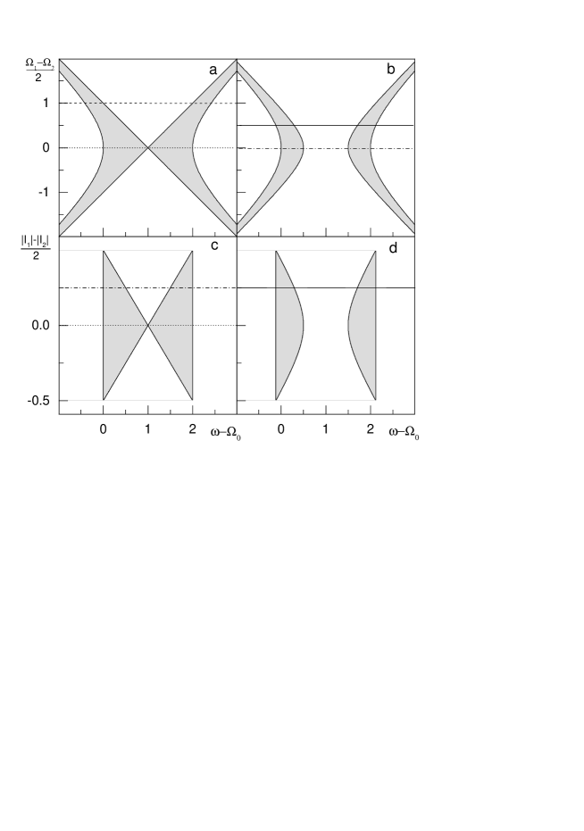
Figure 1: FIGURE 1.

Let us discuss the results for the density of states for the considered periodic nonuniform chains. The main consequence of introducing the nonuniformity is a splitting of the initial magnon band into several subbands (compare (8) and (9) - (13)). The edges of the subbands are determined by the roots of equations ${\cal{B}}(\omega)=0$, ${\cal{C}}(\omega)=0$, ${\cal{D}}(\omega)=0$, etc.. $\rho(\omega)$ is positive inside the subbands, tends to infinity inversely proportionally to the square root of $\omega-\omega_{e}$ when $\omega$ approaches the subbands edges $\omega_{e}$, and is equal to zero outside the subbands. The number of subbands does not exceed the period of the chain. At special (symmetric) values of the Hamiltonian parameters the roots of the equation that determines the subband edges may become multiple and the zeros in the denominator and the numerator in the expression for $\rho(\omega)$ may cancel each other. As a result due to an increase of symmetry one may observe a smaller number of subbands. This ‘mechanism’ is easily traced, for example, in formulas (9) - (11) if putting $\Omega_{1}=\Omega_{2}$, $|I_{1}|=|I_{2}|$. The described magnon band structure can be seen in Figs. 1 and 2a, 3 and 4a, and 5 and 6a where we show $\rho(\omega)$ for a few particular periodic nonuniform chains having periods 2, 3, and 12, respectively. The splitting caused by periodic nonuniformity in fact is not surprising. The periodic nonuniform chain is simply another viewpoint on the uniform chain with a crystalline unit cell containing several sites. On the other hand, it is generally known that one may expect several subbands for a crystal having several atoms per unit cell.³⁶

Further one can easily calculate the widths of energy gaps in the magnon spectrum that appear due to nonuniformity. For example, for a chain having a period 2 one finds

$$b_{2}-b_{3}=\sqrt{(\Omega_{1}-\Omega_{2})^{2}+4(|I_{1}|-|I_{2}|)^{2}}.$$ (27)

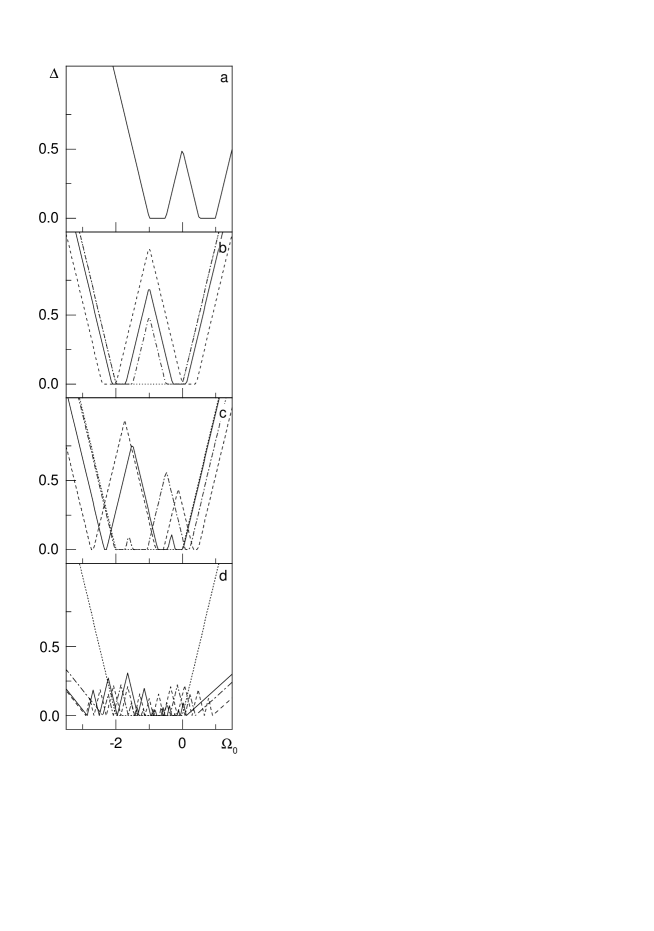
Figure 7: FIGURE 7.

This quantity is connected with a gap between the ground state energy and the first excited state energy of the spin chain. As an example consider the chain $\Omega_{0}I_{1}\Omega_{0}I_{2}\Omega_{0}I_{1}\Omega_{0}I_{2}\ldots\;$. The edges of the upper magnon subband are given by $\Omega_{0}+|I_{1}|+|I_{2}|$ and $\Omega_{0}+||I_{1}|-|I_{2}||$, whereas the edges of the lower magnon subband are given by $\Omega_{0}-||I_{1}|-|I_{2}||$, and $\Omega_{0}-|I_{1}|-|I_{2}|$. At $\Omega_{0}=0$ the ground state (for which $s^{z}=0$) corresponds to the filled lower subband and the empty upper subband and the energy spectrum exhibits a gap $\Delta(0)=||I_{1}|-|I_{2}||$ (this is the energy required to create a hole in the lower subband — the first excited state of the spin chain (with $s^{z}\neq 0$)). With increasing of $\Omega_{0}$ the gap $\Delta$ decreases as $\Delta(\Omega_{0})=||I_{1}|-|I_{2}||-\Omega_{0}$ and becomes zero at $\Omega_{0}=||I_{1}|-|I_{2}||$. With further increasing of $\Omega_{0}$ the gap remains equal to zero up to the value of the transverse field $\Omega_{0}=|I_{1}|+|I_{2}|$ after which the gap opens and increases as $\Delta(\Omega_{0})=\Omega_{0}-|I_{1}|-|I_{2}|$ (the ground state for the transverse field larger than $|I_{1}|+|I_{2}|$ corresponds to the empty subbands and the written $\Delta(\Omega_{0})$ is the energy required to create a particle in the vicinity of the lower edge of the lower subband). For chains with larger periods one finds more complicated behaviour of the energy gap $\Delta$ with varying of the field $\Omega_{0}$ (see Fig. 7a and Figs. 7b - 7d).

The splitting of the magnon band into subbands caused by nonuniformity has interesting consequences for thermodynamic properties. The entropy, specific heat, transverse magnetization and static transverse linear susceptibility are determined through the density of states according to the following formulas

$$s=\int\limits_{-\infty}^{\infty}{\mbox{d}}E\rho(E)\left[\ln\left(2\cosh\frac{E}{2kT}\right)-\frac{E}{2kT}\tanh\frac{E}{2kT}\right],$$ (28)

$$c=\int\limits_{-\infty}^{\infty}{\mbox{d}}E\rho(E)\left(\frac{\frac{E}{2kT}}{\cosh\frac{E}{2kT}}\right)^{2},$$ (29)

$$m_{z}=-\frac{1}{2}\int\limits_{-\infty}^{\infty}{\mbox{d}}E\rho(E)\tanh\frac{E}{2kT},$$ (30)

$$\chi_{zz}=-\frac{1}{kT}\int\limits_{-\infty}^{\infty}{\mbox{d}}E\rho(E)\frac{1}{4\cosh^{2}\frac{E}{2kT}}.$$ (31)

Apparently the most spectacular changes caused by regular nonuniformity are observed in the dependence of transverse magnetization (17) on transverse field at low temperatures (Figs. 2b, 4b, 6b). Since for $T\rightarrow 0$, $\tanh\frac{E}{2kT}$ tends either to $-1$ if $E<0$, or to $1$ if $E>0$, one immediately finds due to the splitting of the magnon band into subbands that the low-temperature dependence of $m_{z}$ versus $\Omega_{0}$ must be composed of sharply increasing parts (they appear when $E=0$ moves with increasing of $\Omega_{0}$ from the bottom to the top of each subband) separated by horizontal parts (they appear when $E=0$ moves with increasing of $\Omega_{0}$ inside the gaps). The number of plateaus is determined by the number of subbands. It should be emphasized here that a study of magnetization plateaus for quantum spin chains is a hot topic at the present time.³⁷ However in such studies usually more general spin chains are attacked which cannot be treated within the frames of the described approach. For example, the spin-$\frac{1}{2}$ $XXX$ chain can be mapped onto the chain of interacting spinless fermions with the intersite interaction of the same order as the hopping integral and hence the results derived rigorously for noninteracting fermions cannot be immediately extended for this more complicated spin chain.

It is interesting to note that the appearance of plateaus in the dependence of transverse magnetization on transverse field at $T=0$ for the regularly nonuniform isotropic $XY$ chains essentially differs in the quantum and classical cases. The Hamiltonian of the classical nonuniform isotropic $XY$ chain in a transverse field reads

$$H=\sum_{n=1}^{N}\Omega_{n}s\cos\theta_{n}+2\sum_{n=1}^{N}I_{n}s^{2}\cos(\phi_{n}-\phi_{n+1})\sin\theta_{n}\sin\theta_{n+1}$$ (32)

that immediately yields the ansatz for the ground state energy in the uniform case

$$E_{0}=N\Omega_{0}s\cos\theta-2N|I|s^{2}\sin^{2}\theta=N\Omega_{0}m_{z}+2N|I|\left(m_{z}^{2}-s^{2}\right)$$ (33)

where the ground state transverse magnetization $m_{z}=s\cos\theta$ has been introduced. Minimizing $E_{0}$ with respect to $\cos\theta$ one finds that for $s=\frac{1}{2}$ the quantity $-m_{z}$ increases as $\frac{1}{2}\frac{\Omega_{0}}{2|I|}$ while $\Omega_{0}$ increases from $0$ to $2|I|$ and $-m_{z}=\frac{1}{2}$ with further increase of $\Omega_{0}$. Using numerical calculations for finite chains (the number of spins $N$ is a multiple of 12) with periods 2, 3, 12 we found that the detailed profiles for the quantum and classical chains are different, although the values of the transverse field at which a saturation of the transverse magnetization occurs are the same. Though one could argue that the magnetization plateaus are connected with the quantum nature of the spins we found for special parameter sets even in the classical chain plateaus in the dependence $-m_{z}$ versus $\Omega_{0}$ (compare dashed curves in Figs. 8a, 8b and in Figs. 2b, 4b). For instance, the well pronounced plateau shown by the dashed line in Fig. 8b occurs at the same height as in the quantum case. The corresponding classical state is a state $\downarrow\uparrow\uparrow\downarrow\uparrow\uparrow\downarrow\uparrow\uparrow\downarrow\uparrow\uparrow\ldots$ where the arrows symbolize classical spins pointing either in $-z$- or $+z$-direction. An evident difference between the quantum and classical case is connected with the slope of the $m_{z}(\Omega_{0})$ curve at $T=0$. The slope remains finite in the classical case but becomes infinite approaching the plateaus in the quantum case. The infinite slope in the quantum case is clearly a consequence of the singularities in the density of states.

One of the interesting magnetic properties of the periodic nonuniform spin-$\frac{1}{2}$ isotropic $XY$ chain is the possibility of the existence of a non-zero transverse magnetization $m_{z}$ at zero average transverse field ($\sum_{n=1}^{N}\Omega_{n}=0$). For illustration we consider as an example a chain having the period 4 and the parameters $\Omega_{1}=\Omega_{3}=0$, $\Omega_{2}=-\Omega_{4}<0$, $|I_{1}|=|I_{2}|>0$, $|I_{3}|=|I_{4}|=0$. At site $n+1$ we have the transverse field $\Omega_{2}<0$ surrounded on the left and right side by the strong couplings $|I_{1}|=|I_{2}|$. At site $n+3$ we have the transverse field $-\Omega_{2}>0$ surrounded by the weak couplings $|I_{3}|=|I_{4}|=0$. One may expect that the local transverse magnetization at site $n+1$ has a smaller value and opposite direction with respect to that quantity at site $n+3$ and therefore a non-zero total transverse magnetization at zero average transverse field may be expected. Consider the described chain in more detail. From Eq. (13) for the above set of parameters it follows that

$$\rho(\omega)=\lambda_{1}\delta\left(\omega-\frac{\Omega_{2}-\sqrt{\Omega_{2}^{2}+8I_{1}^{2}}}{2}\right)+\lambda_{2}\delta\left(\omega\right)+\lambda_{3}\delta\left(\omega-\frac{\Omega_{2}+\sqrt{\Omega_{2}^{2}+8I_{1}^{2}}}{2}\right)+\lambda_{4}\delta\left(\omega+\Omega_{2}\right)$$ (34)

and the coefficients $\lambda_{j}$ may be found comparing (21) and (13) in the vicinity of $\frac{\Omega_{2}-\sqrt{\Omega_{2}^{2}+8I_{1}^{2}}}{2}$, $0$, $\frac{\Omega_{2}+\sqrt{\Omega_{2}^{2}+8I_{1}^{2}}}{2}$ and $-\Omega_{2}$. As a result one gets $\lambda_{j}=\frac{1}{4}$ (see Fig. 9a). Now transverse magnetization (17) at $T=0$ is $m_{z}=-\frac{1}{8}\neq 0$ although $\sum_{n=1}^{N}\Omega_{n}=0$ (solid curves in Figs. 9b, 9c; in the latter figure the solid curve especially clearly shows that $-m_{z}=\frac{1}{8}$). If $|I_{3}|=|I_{4}|\neq 0$ the magnon subbands look as in Fig. 9a and at $T=0$ one has $m_{z}=0$ (Figs. 9b, 9c). However, such a position of the subbands provides an interesting temperature dependence of $m_{z}$ at $\sum_{n=1}^{N}\Omega_{n}=0$ (dashed and dotted curves in Fig. 9c) reminding the ‘order from disorder’ phenomenon,^38-40 i.e. increasing of order with increasing temperature.

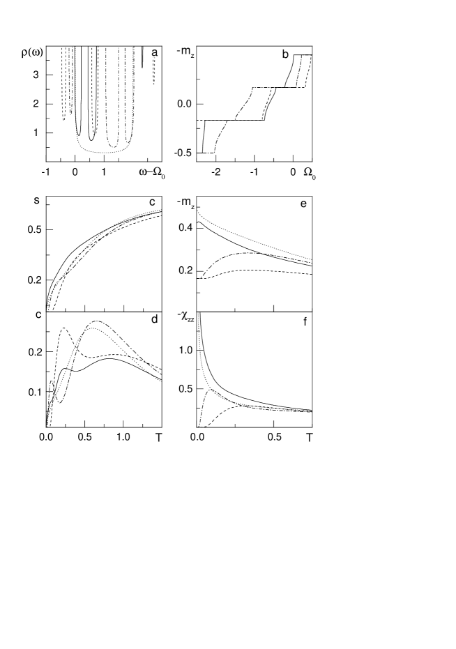
Figure 4: FIGURE 4.

Let us turn to other thermodynamic quantities. Every infinite slope in the dependence $m_{z}$ versus $\Omega_{0}$ at $T=0$ induces a singularity in the dependence $\chi_{zz}$ versus $\Omega_{0}$ at $T=0$. However, there is no need to plot this dependence. Since $1/4kT\cosh^{2}\frac{E}{2kT}$ tends to $\delta(E)$ as $T\to 0$ one gets from (18) that at $T=0$   $-\chi_{zz}=\rho(0)$. The latter dependence as a matter of fact can be seen in Figs. 2a, 4a, 6a. The changes in the temperature dependences of entropy and specific heat due to nonuniformity which are displayed in Figs. 2c, 4c, 6c and 2d, 4d, 6d can be understood while bearing in mind the behaviour of integrands in (15), (16) that are products of the functions with evident dependences on the temperature and the density of states. Note that as a result of the magnon band splitting the temperature dependence of the specific heat may exhibit a two-peak structure (Fig. 2d) or even a more complicated behaviour (solid curve in Fig. 4d). Finally we look at $\chi_{zz}$. As mentioned above at $T=0$ we have   $-\chi_{zz}=\rho(0)$. Analysing the density of states depicted in Figs. 2a, 4a, 6a one finds that nonuniformity may either suppress or enhance the initial (that is at $\Omega_{0}=0$) static transverse linear susceptibility $-\chi_{zz}$ at $T=0$ shown in Figs. 2f, 4f, 6f.

3 Periodic nonuniform spin-$\frac{1}{2}$ isotropic $XY$ chain in a random Lorentzian transverse field

In this Section we consider a generalization of model (1) including additional randomness in the transverse fields. We assume the transverse fields to be independent random variables each with a Lorentzian probability distribution

$$p(\Omega_{n})=\frac{1}{\pi}\frac{\Gamma_{n}}{\left(\Omega_{0n}-\Omega_{n}\right)^{2}+\Gamma_{n}^{2}}.$$ (35)

Here $\Omega_{0n}$ is the mean value of the transverse field at site $n$ and $\Gamma_{n}$ is the width of its distribution. We are interested in the random-averaged density of states $\overline{\rho(\omega)}$ that follows from the random-averaged diagonal Green functions $\overline{G_{nn}^{\mp}}$ according to Eq. (4). Repeating the arguments presented in Refs. 6-11 one gets the following set of equations for the random-averaged Green functions

$$\left(\omega\pm{\mbox{i}}\Gamma_{n}-\Omega_{0n}\right)\overline{G_{nm}^{\mp}}-I_{n-1}\overline{G_{n-1,m}^{\mp}}-I_{n}\overline{G_{n+1,m}^{\mp}}=\delta_{nm}$$ (36)

that immediately yields

$$\overline{G_{nn}^{\mp}}=\frac{1}{\omega\pm{\mbox{i}}\Gamma_{n}-\Omega_{0n}-\Delta^{-}_{n}-\Delta^{+}_{n}},$$

$$\Delta^{-}_{n}=\frac{I_{n-1}^{2}}{\omega\pm{\mbox{i}}\Gamma_{n-1}-\Omega_{0,n-1}-\frac{I_{n-2}^{2}}{\omega\pm{\mbox{i}}\Gamma_{n-2}-\Omega_{0,n-2}-_{\ddots}}},$$

$$\Delta^{+}_{n}=\frac{I_{n}^{2}}{\omega\pm{\mbox{i}}\Gamma_{n+1}-\Omega_{0,n+1}-\frac{I_{n+1}^{2}}{\omega\pm{\mbox{i}}\Gamma_{n+2}-\Omega_{0,n+2}-_{\ddots}}}.$$ (37)

In case $\Omega_{0n},$ $\Gamma_{n},$ $I_{n}$ vary regularly from site to site one again comes to the periodic continued fractions. They can be calculated as solutions of the corresponding quadratic equations. Thus one gets rigorously the random-averaged Green functions and therefore the random-averaged density of states. For example, for a regular random chain $\Omega_{01}\Gamma_{1}I_{1}\Omega_{02}\Gamma_{2}I_{2}\Omega_{01}\Gamma_{1}I_{1}\Omega_{02}\Gamma_{2}I_{2}\ldots$ one finds

$$\overline{\rho(\omega)}=\frac{1}{2\pi}\frac{|{\cal{Y}}(\omega)|}{{\cal{B}}(\omega)};$$

$${\cal{Y}}(\omega)=(\Gamma_{1}+\Gamma_{2})\sqrt{\frac{{\cal{B}}(\omega)+{\cal{B}}^{\prime}(\omega)}{2}}-{\mbox{sgn}}{\cal{B}}^{\prime\prime}(\omega)(2\omega-\Omega_{01}-\Omega_{02})\sqrt{\frac{{\cal{B}}(\omega)-{\cal{B}}^{\prime}(\omega)}{2}},$$

$${\cal{B}}(\omega)=\sqrt{\left({\cal{B}}^{\prime}(\omega)\right)^{2}+\left({\cal{B}}^{\prime\prime}(\omega)\right)^{2}},$$

$${\cal{B}}^{\prime}(\omega)=\left[(\omega-\Omega_{01})(\omega-\Omega_{02})-\Gamma_{1}\Gamma_{2}-I_{1}^{2}-I_{2}^{2}\right]^{2}-\left[(\omega-\Omega_{01})\Gamma_{2}+(\omega-\Omega_{02})\Gamma_{1}\right]^{2}-4I_{1}^{2}I_{2}^{2},$$

$${\cal{B}}^{\prime\prime}(\omega)=2\left[(\omega-\Omega_{01})(\omega-\Omega_{02})-\Gamma_{1}\Gamma_{2}-I_{1}^{2}-I_{2}^{2}\right]\left[(\omega-\Omega_{01})\Gamma_{2}+(\omega-\Omega_{02})\Gamma_{1}\right].$$ (38)

The random-averaged density of states (25) transforms into (9) if $\Gamma_{1}=\Gamma_{2}=0$, and into the result reported in Ref. 9, $\overline{\rho(\omega)}=\mp(1/\pi){\mbox{Im}}1/\sqrt{(\omega\pm{\mbox{i}}\Gamma-\Omega_{0})^{2}-4I^{2}},$ if $\Omega_{01}=\Omega_{02}=\Omega_{0},$ $\Gamma_{1}=\Gamma_{2}=\Gamma,$ $I_{1}=I_{2}=I.$

Let us discuss the effects of the considered diagonal Lorentzian disorder. The main effect of the randomness is smearing out the band structure. However, one can see a difference in smoothed magnon subbands for the uniform disorder (when $\Gamma_{1}=\Gamma_{2}$) (see Fig. 10a) and the nonuniform disorder (when $\Gamma_{1}\neq\Gamma_{2}$) (see Fig. 11a). Namely, in the former case both subbands are smeared out in the same way, whereas in the latter case, the subbands are smeared out differently and, at least for small strengths of disorder, in one subband the peaks at the band edges persist. This circumstance in the latter case induces an interesting step-like behaviour of the low-temperature transverse magnetization as a function of transverse field. Namely, as can be seen in Fig. 11b the disorder smooths only one step in contrast to Fig. 10b in which both steps are smeared out. The difference in the influence of the uniform and nonuniform disorders on other thermodynamic quantities can be seen in Figs. 10c - 10f and 11c - 11f.

4 Periodic nonuniform spin-$\frac{1}{2}$ isotropic $XY$ chains and spin-Peierls instability

In this Section we want to demonstrate that the results for the density of states of the periodic nonuniform spin-$\frac{1}{2}$ isotropic $XY$ chains obtained within the continued-fraction approach may be of use for the study of the spin-Peierls instability in these chains in adiabatic limit. The discovery of existence of the spin-Peierls transition in the inorganic compound CuGeO₃^41,42 has stimulated much research work in this field. In particular, the influence of an external field or randomness attracts much interest both from experimental and theoretical viewpoints (see e.g. Refs. 42-49).

Let us start from the non-random case. In order to examine the instability of the spin chain with respect to dimerization one must calculate the ground state energy per site of the regularly alternating chain $\Omega_{1}I_{1}\Omega_{2}I_{2}\Omega_{1}I_{1}\Omega_{2}I_{2}\ldots$ (see Eqs. (9) - (11))

$$e_{0}=-\frac{1}{2}\int\limits_{-\infty}^{\infty}{\mbox{d}}E\rho(E)|E|=-\frac{1}{2\pi}\int\limits_{-{\sf{b}}_{1}}^{-{\sf{b}}_{2}}{\mbox{d}}E\frac{|E|\left(|E-\hat{\Omega}|+|E+\hat{\Omega}|\right)}{\sqrt{-\left(E^{2}-{\sf{b}}_{1}^{2}\right)\left(E^{2}-{\sf{b}}_{2}^{2}\right)}}$$ (39)

where $\hat{\Omega}=(\Omega_{1}+\Omega_{2})/2$. Depending on the value of $\hat{\Omega}$ formula (26) can be rewritten as follows

$$e_{0}=-\frac{1}{\pi}\int\limits_{-{\sf{b}}_{1}}^{-{\sf{b}}_{2}}{\mbox{d}}E\frac{|\hat{\Omega}||E|}{\sqrt{-\left(E^{2}-{\sf{b}}_{1}^{2}\right)\left(E^{2}-{\sf{b}}_{2}^{2}\right)}}$$ (40)

if ${\sf{b}}_{1}\leq|\hat{\Omega}|$,

$$e_{0}=-\frac{1}{\pi}\int\limits^{-|\hat{\Omega}|}_{-{\sf{b}}_{1}}{\mbox{d}}E\frac{E^{2}}{\sqrt{-\left(E^{2}-{\sf{b}}_{1}^{2}\right)\left(E^{2}-{\sf{b}}_{2}^{2}\right)}}-\frac{1}{\pi}\int\limits_{-|\hat{\Omega}|}^{-{\sf{b}}_{2}}{\mbox{d}}E\frac{|\hat{\Omega}||E|}{\sqrt{-\left(E^{2}-{\sf{b}}_{1}^{2}\right)\left(E^{2}-{\sf{b}}_{2}^{2}\right)}}$$ (41)

if ${\sf{b}}_{2}\leq|\hat{\Omega}|<{\sf{b}}_{1}$, and

$$e_{0}=-\frac{1}{\pi}\int\limits_{-{\sf{b}}_{1}}^{-{\sf{b}}_{2}}{\mbox{d}}E\frac{E^{2}}{\sqrt{-\left(E^{2}-{\sf{b}}_{1}^{2}\right)\left(E^{2}-{\sf{b}}_{2}^{2}\right)}}$$ (42)

if $|\hat{\Omega}|<{\sf{b}}_{2}$. Introducing a new variable $\varphi$ by the relation $E=-\sqrt{{\sf{b}}_{1}^{2}-({\sf{b}}_{1}^{2}-{\sf{b}}_{2}^{2})\sin^{2}\varphi}$ one gets the following final expression for the ground state energy

$$e_{0}=-\frac{1}{\pi}\left[{\sf{b}}_{1}{\mbox{E}}\left(\psi,\frac{{\sf{b}}_{1}^{2}-{\sf{b}}_{2}^{2}}{{\sf{b}}_{1}^{2}}\right)+|\hat{\Omega}|\left(\frac{\pi}{2}-\psi\right)\right]$$ (43)

where ${\mbox{E}}(\psi,a^{2})=\int_{0}^{\psi}{\mbox{d}}\varphi\sqrt{1-a^{2}\sin^{2}\varphi}$ is the elliptic integral of the second kind⁵⁰ and

$$\psi=\left\{\begin{array}[]{ll}0,&{\mbox{if}}\;\;\;{\sf{b}}_{1}\leq|\hat{\Omega}|,\\ {\mbox{arcsin}}\sqrt{\frac{{\sf{b}}_{1}^{2}-\hat{\Omega}^{2}}{{\sf{b}}_{1}^{2}-{\sf{b}}_{2}^{2}}},&{\mbox{if}}\;\;\;{\sf{b}}_{2}\leq|\hat{\Omega}|<{\sf{b}}_{1},\\ \frac{\pi}{2},&{\mbox{if}}\;\;\;|\hat{\Omega}|<{\sf{b}}_{2}.\end{array}\right.$$ (47)

The result obtained by Pincus¹³ follows from (30), (31) if $\Omega_{1}=\Omega_{2}=0$. However, the described approach permits to get the ground state energy (or the Helmholtz free energy) for more complicated regular nonuniformities (e.g., for chains with regularly alternating non-random or random (Lorentzian) transverse fields). To demonstrate this let us consider at first the spin-Peierls instability with respect to dimerization in the presence of a non-random transverse field. We introduce dimerization parameter $\delta$ and assume in (30), (31) $|I_{1}|=|I|(1+\delta)$, $|I_{2}|=|I|(1-\delta)$, $0\leq\delta\leq 1$. Taking into account that the elastic energy per site is $\alpha\delta^{2}$ one must seek the minimum of the total energy ${\cal{E}}(\delta)=e_{0}(\delta)+\alpha\delta^{2}$ as a function of $\delta$. For ${\cal{E}}(\delta)$ we find

$${\cal{E}}(\delta)=-\frac{\sqrt{(\Omega_{1}-\Omega_{2})^{2}+16I^{2}}}{2\pi}{\mbox{E}}\left(\psi,\frac{4I^{2}(1-\delta^{2})}{\frac{1}{4}(\Omega_{1}-\Omega_{2})^{2}+4I^{2}}\right)-|\Omega_{1}+\Omega_{2}|\left(\frac{1}{4}-\frac{\psi}{2\pi}\right)+\alpha\delta^{2}$$ (48)

with

$$\psi=\left\{\begin{array}[]{ll}0,&{\mbox{if}}\;\;\;\sqrt{(\Omega_{1}-\Omega_{2})^{2}+16I^{2}}\leq|\Omega_{1}+\Omega_{2}|,\\ {\mbox{arcsin}}\sqrt{\frac{4I^{2}-\Omega_{1}\Omega_{2}}{4I^{2}(1-\delta^{2})}},&{\mbox{if}}\;\;\;\sqrt{(\Omega_{1}-\Omega_{2})^{2}+16I^{2}\delta^{2}}\leq|\Omega_{1}+\Omega_{2}|<\sqrt{(\Omega_{1}-\Omega_{2})^{2}+16I^{2}},\\ \frac{\pi}{2},&{\mbox{if}}\;\;\;|\Omega_{1}+\Omega_{2}|<\sqrt{(\Omega_{1}-\Omega_{2})^{2}+16I^{2}\delta^{2}}.\end{array}\right.$$ (52)

Eqs. (32), (33) in the limit of uniform field $\Omega_{1}=\Omega_{2}$ coincide with the result reported in Ref. 16. For strong fields $|\Omega_{1}+\Omega_{2}|\geq\sqrt{(\Omega_{1}-\Omega_{2})^{2}+16I^{2}}$ one finds that ${\cal{E}}(\delta)=-\frac{1}{4}|\Omega_{1}+\Omega_{2}|+\alpha\delta^{2}$ and the equation $\frac{\partial{\cal{E}}(\delta)}{\partial\delta}=0$ has only the zero solution $\delta^{\star}=0$ (no dimerization in strong enough fields), whereas for weaker fields besides the zero solution there may be a non-zero one $\delta^{\star}\neq 0$ coming from the equation

$$\alpha=\frac{\sqrt{(\Omega_{1}-\Omega_{2})^{2}+16I^{2}}}{4\pi(1-\delta^{2})}\left[{\mbox{F}}\left(\psi,\frac{4I^{2}(1-\delta^{2})}{\frac{1}{4}(\Omega_{1}-\Omega_{2})^{2}+4I^{2}}\right)-{\mbox{E}}\left(\psi,\frac{4I^{2}(1-\delta^{2})}{\frac{1}{4}(\Omega_{1}-\Omega_{2})^{2}+4I^{2}}\right)\right]$$ (53)

where ${\mbox{F}}(\psi,a^{2})=\int_{0}^{\psi}{\mbox{d}}\varphi/\sqrt{1-a^{2}\sin^{2}\varphi}$ is the elliptic integral of the first kind.⁵⁰

In the following discussion of results we choose a uniform transverse field $\Omega_{1}=\Omega_{2}=\Omega_{0}$, $|\Omega_{0}|<2|I|$. To give a guide for further reading this paragraph we summarize the main results valid for sufficiently hard lattices (having $\alpha>\frac{|I|}{4}$). (i) For zero field we have a minimum of the total energy ${\cal{E}}(\delta)$ at a nonzero value of the dimerization parameter $\delta^{\star}\neq 0$. (ii) For finite but small fields ${\cal{E}}(\delta)$ still exhibits one minimum at $\delta^{\star}\neq 0$ the position of which remains unchanged. (iii) When the field achieves a certain characteristic value $\Omega_{0a}$ a second local minimum appears at $\delta^{\star}=0$. The two minima at $\delta^{\star}=0$ and $\delta^{\star}\neq 0$ are separated by a maximum. (iv) At a second characteristic field $\Omega_{0b}$ both minima at $\delta^{\star}=0$ and $\delta^{\star}\neq 0$ have the same depth. (v) Further increasing $\Omega_{0}$ the minimum at $\delta^{\star}=0$ becomes the global one and at a certain characteristic field $\Omega_{0c}$ the minimum at $\delta^{\star}\neq 0$ abruptly disappears. The scenario described in (i) – (v) is typical for a first order transition characterized by the order parameter $\delta^{\star}$ and driven by the transverse field $\Omega_{0}$. Now we illustrate it in a more detail.

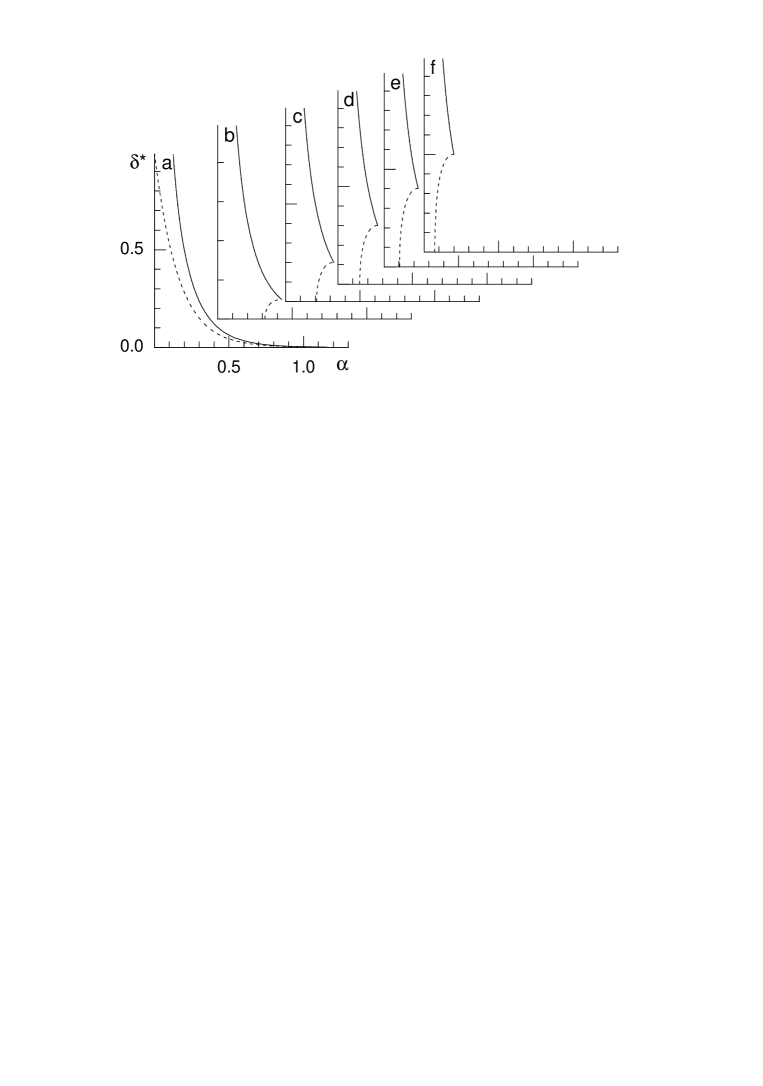
Figure 13: FIGURE 13.

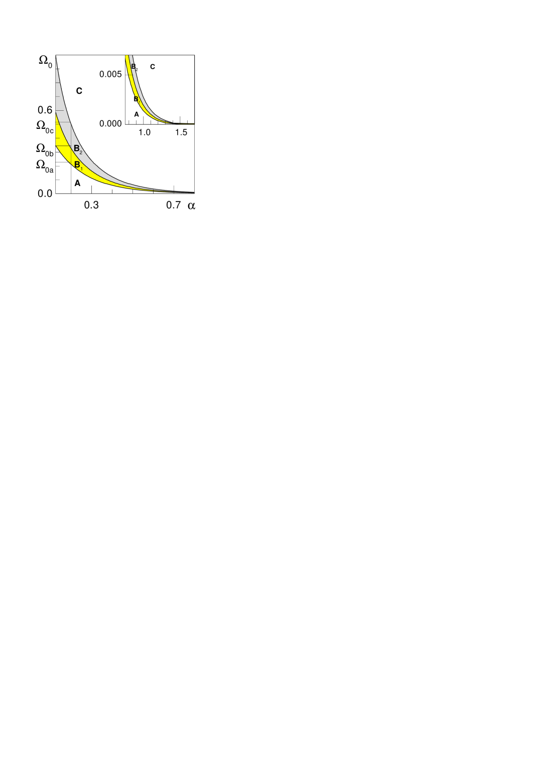
Figure 14: FIGURE 14.

In Fig. 12 we show for different values of $\alpha$ how the dependence of ${\cal{E}}(\delta)-{\cal{E}}(0)$ on the dimerization parameter varies with the strength of the field $\Omega_{0}$. As it follows from Eqs. (32), (33) (and can be also seen in Fig. 12 where, however, the difference ${\cal{E}}(\delta)-{\cal{E}}(0)$ is depicted) the total energy ${\cal{E}}(\delta)$ at sufficiently large values of $\delta$ ($\delta\geq\frac{|\Omega_{0}|}{2|I|}$, ${\cal{E}}(\delta)-{\cal{E}}(0)$ at the value $\frac{|\Omega_{0}|}{2|I|}$ is denoted by dark circles in Fig. 12) becomes independent of the field. In Fig. 13 we plot the solution of Eqs. (34), (33) for different lattices (i.e. different values of $\alpha$) in the presence of the field. As a matter of fact we calculated r.h.s. of Eq. (34) varying $\delta$ from 0 to 1 and finding in such a way for what $\alpha$ this value of $\delta^{\star}$ realizes. Note that solutions of Eqs. (34), (33) $\delta^{\star}$ which are smaller than $\frac{|\Omega_{0}|}{2|I|}$ realize a maximum of the total energy, whereas solutions $\delta^{\star}$ which are larger than $\frac{|\Omega_{0}|}{2|I|}$ realize a minimum. This can be seen, for example, for a lattice with $\alpha=0.4$ in Figs. 12c and 13b, 13c: at $\Omega_{0}=0.1$ the total energy ${\cal{E}}(\delta)$ exhibits two minima at $\delta^{\star}=0$ and $\delta^{\star}\neq 0$ separated by a maximum at intermediate value of $\delta^{\star}$; at $\Omega_{0}=0.2$ the total energy ${\cal{E}}(\delta)$ exhibits only a minimum at $\delta^{\star}=0$. From Figs. 12, 13 and Eqs. (34), (33) one concludes that for soft lattices having $\alpha<\frac{|I|}{4}$ there is no solution of Eqs. (34), (33) fulfilling the presupposition $\delta^{\star}\leq 1$. Such lattices are excluded from further consideration. For other lattices the solution of Eqs. (34), (33) $\delta^{\star}\neq 0$ existing for zero transverse field does not feel the presence of a small field, however, abruptly vanishes at a certain value of the transverse field. Moreover, for soft lattices one needs larger fields than for hard lattices for a disappearance of the solution of Eqs. (34), (33) (compare Figs. 13b - 13f with Fig. 13a). Thus, in the case of hard lattices even small transverse fields may destroy the dimerization. As it is seen e.g. for a lattice with $\alpha=0.2$ (Figs. 12, 13) above a certain characteristic value of the transverse field $\Omega_{0a}$ (for which Eqs. (34), (33) has the solution $\delta^{\star}=0$) ($\Omega_{0a}\approx 0.2$) ${\cal{E}}(\delta)$ starts to exhibit in addition to the global minimum at $\delta^{\star}\neq 0$, a local one at $\delta^{\star}=0$, two minima are separated by a maximum at the intermediate value of the dimerization parameter. With increasing of $\Omega_{0}$ the depths of the minima at first become equal (when $\Omega_{0}$ has a characteristic value $\Omega_{0b}$) and then the minima at $\delta^{\star}=0$ becomes a global one. The latter minima remains the only one at $\Omega_{0}$ having a characteristic value $\Omega_{0c}$ (for which Eqs. (34), (33) has the solution $\delta^{\star}=\frac{|\Omega_{0}|}{2|I|}$) ($\Omega_{0c}\approx 0.5$) that manifests a complete suppression of the dimerization by the field. In Fig. 14 we show different regions in the plane transverse field $\Omega_{0}$ – lattice parameter $\alpha$ in which ${\cal{E}}(\delta),$ $0\leq\delta\leq 1$ exhibits one minimum at $\delta^{\star}\neq 0$ (region A), two minima at $\delta^{\star}=0$ and $\delta^{\star}\neq 0$ separated by a maximum (regions B₁ and B₂; in the region B₁ the minimum at $\delta^{\star}\neq 0$ is deeper, whereas in the region B₂ the minimum at $\delta^{\star}=0$ is deeper), one minimum at $\delta^{\star}=0$ (region C). To find the line that separates B₁ and B₂ one must find for a given $\Omega_{0}$ such a $\delta^{\star}$ at which ${\cal{E}}(\delta)-{\cal{E}}(0)$ (32), (33) with $\alpha$ given by the r.h.s. of Eq. (34), (33) equals to zero, and then to evaluate the r.h.s. of Eq. (34) at the sought $\delta^{\star}$. Crossing the phase diagram by a vertical line corresponding to a certain lattice (e.g. with $\alpha=0.2$ in Fig. 14) one obtains the field at which the first order transition between the dimerized and uniform phases occur ($\Omega_{0b}$ in Fig. 14) and the width of hysteresis (determined by $\Omega_{0a}$ and $\Omega_{0c}$ in Fig. 14).

Next we consider the influence of a random Lorentzian transverse field on the spin-Peierls instability with respect to dimerization. For that we calculate the difference in random-averaged total energy (to avoid non-physical infinities due to the Lorentzian probability distribution)

$$\overline{{\cal{E}}(\delta)}-\overline{{\cal{E}}(0)}=-\frac{1}{2}\int\limits_{-\infty}^{\infty}{\mbox{d}}E\left(\overline{\rho_{\delta}(E)}-\overline{\rho_{0}(E)}\right)|E|+\alpha\delta^{2}$$ (54)

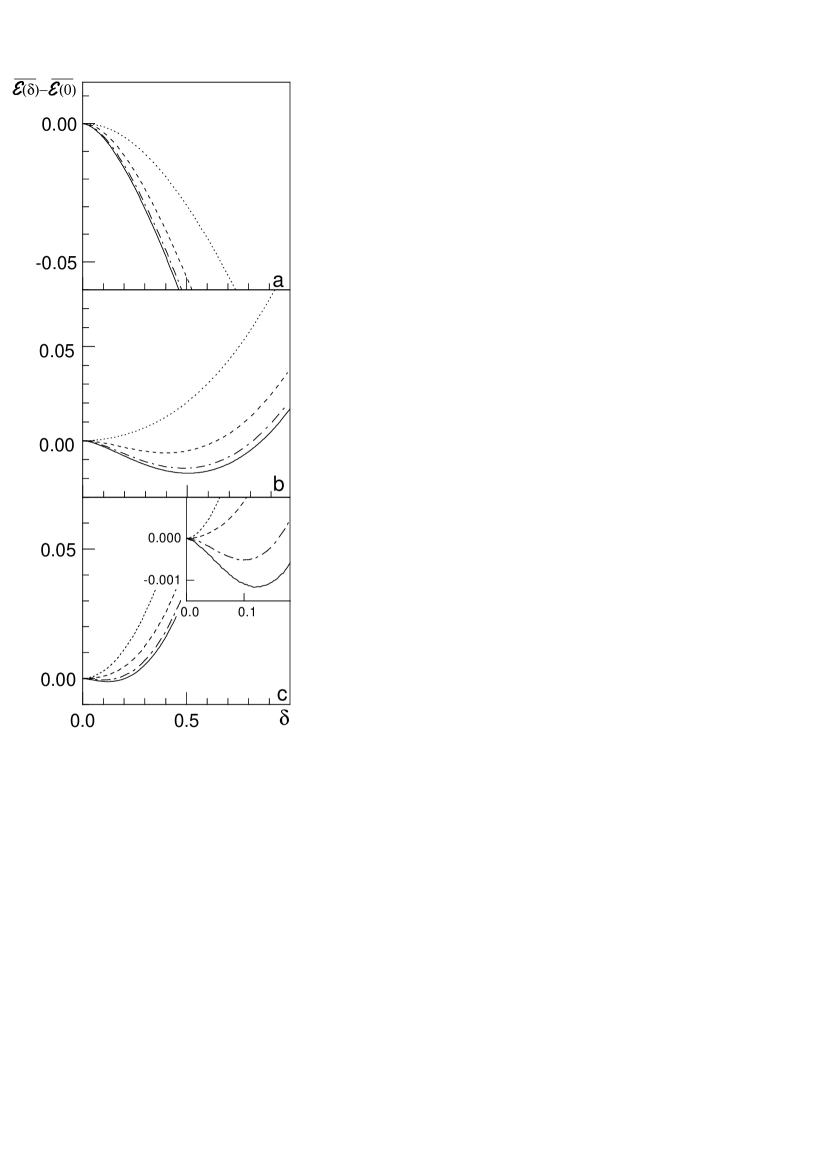
Figure 15: FIGURE 15.

with $\overline{\rho_{\delta}(E)}$ given by Eq. (26) where $|I_{1}|=|I|(1+\delta)$, $|I_{2}|=|I|(1-\delta)$. Let us start from the case $\Omega_{01}=\Omega_{02}=0$, $\Gamma_{1}=\Gamma_{2}=\Gamma$ generalizing in such a way the consideration for the zero transverse field by assuming the latter to be random (Lorentzian) with the zero mean value. As can be seen in Fig. 15 the randomness leads to a continuous decrease of the non-zero value of dimerization parameter at which the random-averaged total energy exhibits minimum. At sufficiently large strengths of disorder $\Gamma$ the minimum of the random-averaged total energy occurs already at the zero dimerization parameter, i.e. randomness acts against dimerization and may suppress it completely for sufficiently large strength of disorder. Considering the equation

$$\frac{\partial\overline{{\cal{E}}(\delta)}}{\partial\delta}=-\frac{1}{2}\int\limits_{-\infty}^{\infty}{\mbox{d}}E\frac{\partial\overline{\rho_{\delta}(E)}}{\partial\delta}|E|+2\alpha\delta=0$$ (55)

one can find its solution $\delta^{\star}$ for different $\Gamma$ (see Fig. 16). From Fig. 16 one sees that in the case of hard lattices even small disorder may destroy the dimerization. In Fig. 17 we depicted different regions in the plane strength of disorder $\Gamma$ – lattice parameter $\alpha$ in which $\overline{{\cal{E}}(\delta)}-\overline{{\cal{E}}(0)}$, $0\leq\delta\leq 1$ exhibits one minimum at $\delta^{\star}\neq 0$ (region A) or one minimum at $\delta^{\star}=0$ (region C). The boundary curve between the regions C and A is obtained by calculating $\alpha$ from (36) with varying $\Gamma$ for fixed $\delta=0$. Thus, the random field with zero mean value suppresses dimerization with increasing the strength of disorder, however the dimerization parameter $\delta^{\star}$ vanishes according to a second order phase transition scenario in contrast to the previous case.

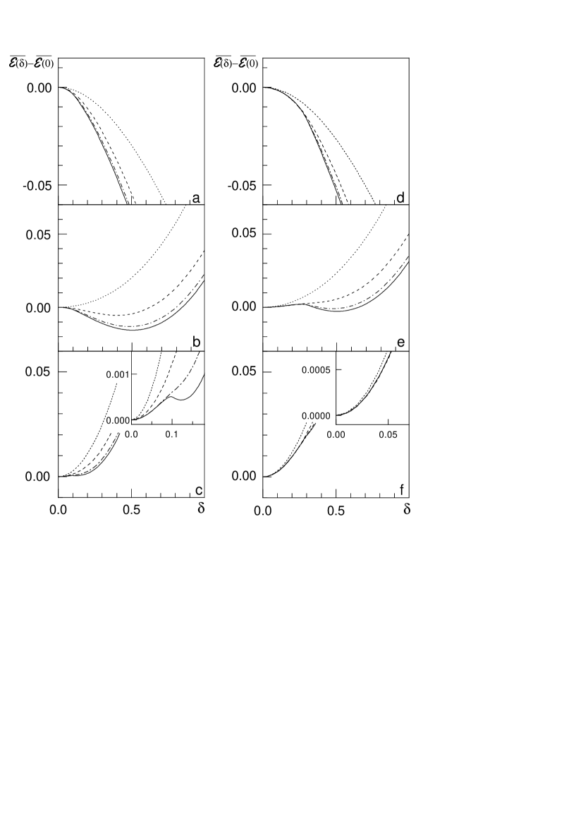
Figure 18: FIGURE 18.

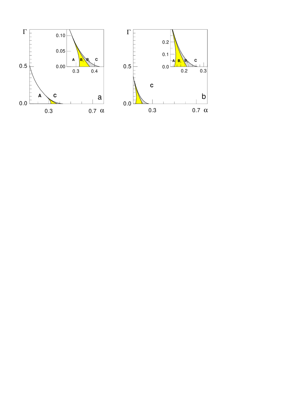
Figure 20: FIGURE 20.

Finally we consider the case of random field with non-zero average value, i.e., $\Omega_{01}=\Omega_{02}=\Omega_{0}\neq 0$, $\Gamma_{1}=\Gamma_{2}=\Gamma$. For small strengths of randomness $\Gamma$ the above discussed scenario of one or two minimum in $\overline{{\cal{E}}(\delta)}$ in dependence of the value of the field remains valid. A switching on randomness for a system being in the region A at $\Gamma=0$ (Fig. 14) leads to continuous decreasing of $\delta^{\star}\neq 0$ to zero. For a system being in the regions B₁ or B₂ an increasing of randomness usually leads at first to a continuous decrease of $\delta^{\star}\neq 0$ with a decrease of the depth of that minimum and then to an abrupt disappearance of $\delta^{\star}\neq 0$ above a certain strength of disorder. We also observed another influence of small randomness for a system being in the region B₁, namely, an increasing of randomness leads at first to a disappearance of the minimum at $\delta^{\star}=0$ that appears again for larger strength of disorder. The details can be traced in Fig. 18 where we plotted the dependence $\overline{{\cal{E}}(\delta)}-\overline{{\cal{E}}(0)}$ vs $\delta$ for different $\Gamma$ considering two mean values of the random transverse field $\Omega_{0}=0.1$ and $\Omega_{0}=0.3$ and in Fig. 19 where we illustrated the vanishing and appearance of the minimum at $\delta^{\star}=0$ with increase of randomness. Both the one minimum profile (solid curve in Fig. 18b) and the two minima profile (solid curves in Figs. 18c, 18e) of that dependence existing in the non-random case $\Gamma=0$ are finally destroyed by increasing disorder. The phase diagrams in the $\Gamma$ – $\alpha$ plane for the two mentioned values of $\Omega_{0}$ are shown in Fig. 20.

Closing this Section, we want to make some comments concerning the conclusions on spin-Peierls instability that can be drawn using exact results for thermodynamic quantities of regularly nonuniform spin-$\frac{1}{2}$ isotropic $XY$ chain in a transverse field. Although the described basic picture of a first order phase transition in a uniform field seems to be qualitatively correct we should keep in mind that an increasing of field at low temperature leads to a transition from dimerized to incommensurate phase. This fact was observed experimentally and analysed theoretically mainly for the models of CuGeO₃ in a number of papers.^42,51-54 Clearly, the simple ansatz for the lattice distortion $\delta_{1}\delta_{2}\delta_{1}\delta_{2}\ldots\;$, $\delta_{1}+\delta_{2}=0$ permitted us to compare the ground state energies only for dimerized and uniform phases. To detect a transition from the dimerized to the incommensurate phase with increasing of field one may analyse the ground state energy of a chain having larger period, say 12. The presence of randomness requires even more complicated lattice distortions to be examined and the continued-fraction approach for rigorous study of thermodynamics of the regularly alternating spin-$\frac{1}{2}$ isotropic $XY$ chain in a transverse field provides some possibilities to perform such an analysis. We must also keep in mind that the known spin-Peierls compounds are described by the spin-$\frac{1}{2}$ isotropic Heisenberg chain rather than $XY$ chain, however, one may expect that the basic features of the studied phenomenon should be similar for both quantum spin models.

5 Summary

To summarize, we have studied rigorously the magnon density of states and the thermodynamics of the periodic nonuniform spin-$\frac{1}{2}$ isotropic $XY$ chain in non-random/random (Lorentzian) transverse field. We have exploited the Jordan-Wigner transformation, the temperature double-time Green functions and the continued fractions. The Green functions approach seems to be the most convenient tool for a study of thermodynamics of the considered spin chains since it permits to examine such models with regular nonuniformity or some type of randomness or both. Regular nonuniformity leads to a splitting of the magnon band into subbands that in its turn leads to some spectacular changes in the behaviour of the gap in the energy spectrum and the thermodynamic quantities. In particular, the low-temperature dependence of the transverse magnetization on the transverse field is composed of sharply increasing parts separated by plateaus, the temperature dependence of specific heat may exhibit a well pronounced two-peak structure, the temperature dependence of the initial transverse linear susceptibility may be enhanced or suppressed. Regularly nonuniform spin-$\frac{1}{2}$ isotropic $XY$ chain may exhibit a non-zero transverse magnetization at the zero average transverse field. The regularly alternating Lorentzian disorder in the transverse field may in specific manner influence the thermodynamic quantities leading, for instance, to a smearing out of only one ‘step’ in the step-like dependence of the transverse magnetization versus the transverse field at $T=0$. The derived results for the (random-averaged) ground state energy permit to analyse the effects of external non-random/random field on the spin-Peierls instability. Both, magnetic field as well as randomness may destroy the dimerization as the analysis of the (random-averaged) total energy manifests.

The presented treatment of the regularly periodic spin-$\frac{1}{2}$ isotropic $XY$ chains is restricted to the density of states and therefore only to thermodynamics. It will be interesting to study the effects of periodic nonuniformity on spin correlations and their dynamics especially for a model of spin-Peierls instability. Some work for the dynamic $zz$ spin correlations for such models has been done in Ref. 16. Another interesting problem concerns the treatment of the periodic nonuniform spin-$\frac{1}{2}$ transverse $XY$ chains with an anisotropic exchange coupling (and in particular the extremely anisotropic case, i.e. the spin-$\frac{1}{2}$ transverse Ising chain). Some results for thermodynamics of such regularly nonuniform chains having period 2 were obtained in Refs. 14, 17, 23. Their relation to the spin-Peierls instability seems to be an intriguing issue.

List of figure captions

FIG. 1. Magnon band structure for periodic chains $\Omega_{1}I_{1}\Omega_{2}I_{2}\Omega_{1}I_{1}\Omega_{2}I_{2}\ldots,$ $\Omega_{j}=\Omega_{0}+\Omega_{j}^{\prime}$; the shadowed areas correspond to the allowed magnon energies. a) $\Omega_{1}^{\prime}+\Omega_{2}^{\prime}=2$, $|I_{1}|=|I_{2}|=0.5$; b) $\Omega_{1}^{\prime}+\Omega_{2}^{\prime}=2$, $|I_{1}|=0.75$, $|I_{2}|=0.25$; c) $\Omega_{1}^{\prime}=\Omega_{2}^{\prime}=1$, $|I_{1}|+|I_{2}|=1$; d) $\Omega_{1}^{\prime}=1.5$, $\Omega_{2}^{\prime}=0.5$, $|I_{1}|+|I_{2}|=1$. The horizontal lines single out the following particular chains: $\Omega_{1}^{\prime}=\Omega_{2}^{\prime}=1$, $|I_{1}|=|I_{2}|=0.5$ (dotted curves), $\Omega_{1}^{\prime}=2$, $\Omega_{2}^{\prime}=0$, $|I_{1}|=|I_{2}|=0.5$ (dashed curve), $\Omega_{1}^{\prime}=\Omega_{2}^{\prime}=1$, $|I_{1}|=0.75$, $|I_{2}|=0.25$ (dashed-dotted curves), $\Omega_{1}^{\prime}=1.5$, $\Omega_{2}^{\prime}=0.5$, $|I_{1}|=0.75$, $|I_{2}|=0.25$ (solid curves).

FIG. 2. The density of states (a), the dependence of the transverse magnetization on transverse field at $T=0$ (b), the temperature dependence of the entropy (c), specific heat (d), transverse magnetization (e), and static linear transverse susceptibility (f) at $\Omega_{0}=0$ for periodic chains $\Omega_{1}I_{1}\Omega_{2}I_{2}\Omega_{1}I_{1}\Omega_{2}I_{2}\ldots,$ $\Omega_{j}=\Omega_{0}+\Omega_{j}^{\prime}$. The dotted curves correspond to the uniform case $\Omega_{1}^{\prime}=\Omega_{2}^{\prime}=1$, $|I_{1}|=|I_{2}|=0.5$, the dashed curves correspond to the case $\Omega_{1}^{\prime}=2$, $\Omega_{2}^{\prime}=0$, $|I_{1}|=|I_{2}|=0.5$, the dashed-dotted curves correspond to the case $\Omega_{1}^{\prime}=\Omega_{2}^{\prime}=1$, $|I_{1}|=0.75$, $|I_{2}|=0.25$, and the solid curves correspond to the case $\Omega_{1}^{\prime}=1.5$, $\Omega_{2}^{\prime}=0.5$, $|I_{1}|=0.75$, $|I_{2}|=0.25$.

FIG. 3. Magnon band structure for periodic chains $\Omega_{1}I_{1}\Omega_{2}I_{2}\Omega_{3}I_{3}\Omega_{1}I_{1}\Omega_{2}I_{2}\Omega_{3}I_{3}\ldots,$ $\Omega_{j}=\Omega_{0}+\Omega_{j}^{\prime}$; the shadowed areas correspond to the allowed magnon energies. a) $\Omega_{1}^{\prime}+\Omega_{2}^{\prime}+\Omega_{3}^{\prime}=3$, $\Omega_{1}^{\prime}-2\Omega_{2}^{\prime}+\Omega_{3}^{\prime}=0$, $|I_{1}|=|I_{2}|=|I_{3}|=0.5$; b) $\Omega_{1}^{\prime}+\Omega_{2}^{\prime}+\Omega_{3}^{\prime}=3$, $\Omega_{1}^{\prime}-2\Omega_{2}^{\prime}+\Omega_{3}^{\prime}=1.5$, $|I_{1}|=|I_{2}|=|I_{3}|=0.5$; c) $\Omega_{1}^{\prime}+\Omega_{2}^{\prime}+\Omega_{3}^{\prime}=3$, $\Omega_{1}^{\prime}-2\Omega_{2}^{\prime}+\Omega_{3}^{\prime}=0$, $|I_{1}|=0.75$, $|I_{2}|=0.5$, $|I_{3}|=0.25$; d) $\Omega_{1}^{\prime}+\Omega_{2}^{\prime}+\Omega_{3}^{\prime}=3$, $\Omega_{1}^{\prime}-2\Omega_{2}^{\prime}+\Omega_{3}^{\prime}=1.5$, $|I_{1}|=0.75$, $|I_{2}|=0.5$, $|I_{3}|=0.25$; e) $\Omega_{1}^{\prime}=\Omega_{2}^{\prime}=\Omega_{3}^{\prime}=1$, $|I_{1}|+|I_{2}|+|I_{3}|=1.5$, $|I_{1}|-2|I_{2}|+|I_{3}|=0$; f) $\Omega_{1}^{\prime}=\Omega_{2}^{\prime}=\Omega_{3}^{\prime}=1$, $|I_{1}|+|I_{2}|+|I_{3}|=1.5$, $|I_{1}|-2|I_{2}|+|I_{3}|=0.75$; g) $\Omega_{1}^{\prime}=1.5$, $\Omega_{2}^{\prime}=1$, $\Omega_{3}^{\prime}=0.5$, $|I_{1}|+|I_{2}|+|I_{3}|=1.5$, $|I_{1}|-2|I_{2}|+|I_{3}|=0$; h) $\Omega_{1}^{\prime}=1.5$, $\Omega_{2}^{\prime}=1$, $\Omega_{3}^{\prime}=0.5$, $|I_{1}|+|I_{2}|+|I_{3}|=1.5$, $|I_{1}|-2|I_{2}|+|I_{3}|=0.75$. The horizontal lines single out the following particular chains: $\Omega_{1}^{\prime}=\Omega_{2}^{\prime}=\Omega_{3}^{\prime}=1$, $|I_{1}|=|I_{2}|=|I_{3}|=0.5$ (dotted curves), $\Omega_{1}^{\prime}=2.5$, $\Omega_{2}^{\prime}=0.5$, $\Omega_{3}^{\prime}=0$, $|I_{1}|=|I_{2}|=|I_{3}|=0.5$ (dashed curve), $\Omega_{1}^{\prime}=1$, $\Omega_{2}^{\prime}=0.5$, $\Omega_{3}^{\prime}=1.5$, $|I_{1}|=0.75$, $|I_{2}|=0.5$, $|I_{2}|=0.25$ (dashed-dotted curve), $\Omega_{1}^{\prime}=1.5$, $\Omega_{2}^{\prime}=1$, $\Omega_{3}^{\prime}=0.5$, $|I_{1}|=1$, $|I_{2}|=|I_{3}|=0.25$ (solid curve).

FIG. 4. The same as in Fig. 2 for periodic chains $\Omega_{1}I_{1}\Omega_{2}I_{2}\Omega_{3}I_{3}\Omega_{1}I_{1}\Omega_{2}I_{2}\Omega_{3}I_{3}\ldots,$ $\Omega_{j}=\Omega_{0}+\Omega_{j}^{\prime}.$ The dotted, dashed, dashed-dotted, and solid curves correspond to the cases pointed out in the capture to Fig. 3.

FIG. 5. The same as in Figs. 1, 3 for periodic chains having a period 12, $\Omega_{1}I_{1}\ldots\Omega_{12}I_{12}\Omega_{1}I_{1}\ldots\Omega_{12}I_{12}\ldots,$ $\Omega_{1}=\Omega_{2}=\ldots=\Omega_{6},$ $\Omega_{7}=\Omega_{8}=\ldots=\Omega_{12},$ $I_{1}=I_{2}=\ldots=I_{6},$ $I_{7}=I_{8}=\ldots=I_{12},$ $\Omega_{j}=\Omega_{0}+\Omega_{j}^{\prime}$. a) $\Omega_{1}^{\prime}+\Omega_{7}^{\prime}=2$, $|I_{1}|=|I_{7}|=0.5$; b) $\Omega_{1}^{\prime}+\Omega_{7}^{\prime}=2$, $|I_{1}|=0.75$, $|I_{7}|=0.25$; c) $\Omega_{1}^{\prime}=\Omega_{7}^{\prime}=1$, $|I_{1}|+|I_{7}|=1$; d) $\Omega_{1}^{\prime}=1.5$, $\Omega_{7}^{\prime}=0.5$, $|I_{1}|+|I_{7}|=1$. The horizontal lines single out the following particular chains: $\Omega_{1}^{\prime}=\Omega_{7}^{\prime}=1$, $|I_{1}|=|I_{7}|=0.5$ (dotted curves), $\Omega_{1}^{\prime}=2$, $\Omega_{7}^{\prime}=0$, $|I_{1}|=|I_{7}|=0.5$ (dashed curve), $\Omega_{1}^{\prime}=\Omega_{7}^{\prime}=1$, $|I_{1}|=0.75$, $|I_{7}|=0.25$ (dashed-dotted curves), $\Omega_{1}^{\prime}=1.5$, $\Omega_{7}^{\prime}=0.5$, $|I_{1}|=0.75$, $|I_{7}|=0.25$ (solid curves).

FIG. 6. The same as in Figs. 2, 4 for the chains singled out in Fig. 5.

FIG. 7. The dependence of the energy gap $\Delta$ between the ground state and the first excited state on transverse field $\Omega_{0}$ for certain regularly nonuniform chains. a) The chain $\Omega_{0}I_{1}\Omega_{0}I_{2}\Omega_{0}I_{1}\Omega_{0}I_{2}\ldots\;$, $|I_{1}|=0.75$, $|I_{2}|=0.25$; b) - d) the chains having periods 2, 3, and 12, respectively, with the notations as in Figs. 2, 4, 6.

FIG. 8. The dependence of the transverse magnetization on the transverse field $\Omega_{0}$ at $T=0$ for classical periodic nonuniform isotropic $XY$ chains in a transverse field. a) Chains having a period 2 ($\Omega^{\prime}_{1}=2$, $\Omega^{\prime}_{2}=0$, $|I_{1}|=|I_{2}|=0.5$ (dashed curve), $\Omega^{\prime}_{1}=\Omega^{\prime}_{2}=1$, $|I_{1}|=0.75$, $|I_{2}|=0.25$ (dashed-dotted curve), $\Omega^{\prime}_{1}=1.5$, $\Omega^{\prime}_{2}=0.5$, $|I_{1}|=0.75$, $|I_{2}|=0.25$ (solid curve)); b) chains having a period 3 ($\Omega^{\prime}_{1}=2.5$, $\Omega^{\prime}_{2}=0.5$, $\Omega^{\prime}_{3}=0$, $|I_{1}|=|I_{2}|=|I_{3}|=0.5$ (dashed curve), $\Omega^{\prime}_{1}=1$, $\Omega^{\prime}_{2}=0.5$, $\Omega^{\prime}_{3}=1.5$, $|I_{1}|=0.75$, $|I_{2}|=0.5$, $|I_{3}|=0.25$ (dashed-dotted curve), $\Omega^{\prime}_{1}=1.5$, $\Omega^{\prime}_{2}=1$, $\Omega^{\prime}_{3}=0.5$, $|I_{1}|=1$, $|I_{2}|=|I_{3}|=0.25$ (solid curve)); c) chains having a period 12 ($\Omega^{\prime}_{1}=2$, $\Omega^{\prime}_{7}=0$, $|I_{1}|=|I_{7}|=0.5$ (dashed curve), $\Omega^{\prime}_{1}=\Omega^{\prime}_{7}=1$, $|I_{1}|=0.75$, $|I_{7}|=0.25$ (dashed-dotted curve), $\Omega^{\prime}_{1}=1.5$, $\Omega^{\prime}_{7}=0.5$, $|I_{1}|=0.75$, $|I_{7}|=0.25$ (solid curve)).

FIG. 9. Illustration of the existence of a non-zero transverse magnetization at the zero average transverse field in a chain having period 4. $\Omega^{\prime}_{1}=\Omega^{\prime}_{3}=0$, $\Omega^{\prime}_{2}=-\Omega^{\prime}_{4}=-1$, $|I_{1}|=|I_{2}|=0.5$, $|I_{3}|=|I_{4}|=0$ (solid curves), $|I_{3}|=|I_{4}|=0.05$ (dashed curves), $|I_{3}|=|I_{4}|=0.25$ (dotted curves).

FIG. 10. The random-averaged density of states (a), the dependence of the transverse magnetization on transverse field at $T=0$ (b), the temperature dependence of the entropy (c), specific heat (d), transverse magnetization (e), and static linear transverse susceptibility (f) at $\Omega_{0}=0$ for periodic chains $\Omega_{01}\Gamma_{1}I_{1}\Omega_{02}\Gamma_{2}I_{2}\Omega_{01}\Gamma_{1}I_{1}\Omega_{02}\Gamma_{2}I_{2}\ldots,$ $\Omega_{0j}=\Omega_{0}+\Omega_{j}^{\prime}$, $\Omega_{1}^{\prime}=1.5$, $\Omega_{2}^{\prime}=0.5$, $|I_{1}|=0.75$, $|I_{2}|=0.25$ for the case of uniform disorder $\Gamma_{1}=\Gamma_{2}=\Gamma$. The solid curves correspond to the non-random case $\Gamma=0$; the long-dashed curves correspond to $\Gamma=0.1$; the short-dashed curves correspond to $\Gamma=0.25$; the dotted curves correspond to $\Gamma=0.5$.

FIG. 11. The same as in Fig. 10 for nonuniform disorder $\Gamma_{1}\neq 0$, $\Gamma_{2}=0$. The solid curves correspond to the non-random case $\Gamma_{1}=0$; the long-dashed curves correspond to $\Gamma_{1}=0.1$; the short-dashed curves correspond to $\Gamma_{1}=0.25$; the dotted curves correspond to $\Gamma_{1}=0.5$.

FIG. 12. Change of the total energy ${\cal{E}}(\delta)-{\cal{E}}(0)$ as a function of the dimerization parameter $\delta$ in the presence of the uniform transverse field; $|I|=0.5$; a) $\alpha=0$, b) $\alpha=0.2$, c) $\alpha=0.4$; $\Omega_{0}=0$ (solid curves), $\Omega_{0}=0.1$ (dashed-dotted-dotted curves), $\Omega_{0}=0.2$ (dashed-dotted curves), $\Omega_{0}=0.3$ (dashed curves), $\Omega_{0}=0.4$ (dotted curves).

FIG. 13. Dimerization parameter $\delta^{\star}$ as a function of $\alpha$ in the presence of a uniform transverse field $\Omega_{0}$; $|I|=0.5$; $\Omega_{0}=0$ (a), $\Omega_{0}=0.1$ (b), $\Omega_{0}=0.2$ (c), $\Omega_{0}=0.3$ (d), $\Omega_{0}=0.4$ (e), $\Omega_{0}=0.5$ (f). The solid curves show the solution of Eqs. (34), (33) corresponding to a minimum of the total energy; the dashed curve in (a) corresponds to the dependence $\delta^{\star}$ versus $\alpha$ valid for hard lattices that was obtained in Ref. 13; the dashed curves in (b) - (f) show the solution of Eqs. (34), (33) corresponding to a maximum of the total energy.

FIG. 14. Different types of solution for the dimerization parameter $\delta^{\star}$ ($0\leq\delta^{\star}\leq 1$) in the plane $\Omega_{0}$ – $\alpha$; $|I|=0.5$. Region A: ${\cal{E}}(\delta)$ has one minimum at $\delta^{\star}\neq 0$, regions B₁, B₂: ${\cal{E}}(\delta)$ has two minima at $\delta^{\star}=0$ (favourable in B₂) and $\delta^{\star}\neq 0$ (favourable in B₁) separated by a maximum, moreover, the depths of the minima at the line that separates B₁ and B₂ are the same; region C: ${\cal{E}}(\delta)$ has one minimum at $\delta^{\star}=0$.

FIG. 15. Change of the random-averaged total energy as a function of the dimerization parameter in the presence of a uniform random Lorentzian transverse field with zero mean value; $|I|=0.5$, $\Gamma_{1}=\Gamma_{2}=\Gamma=0$ (solid curves), $\Gamma=0.02$ (dashed-dotted curves), $\Gamma=0.1$ (dashed curves), $\Gamma=0.5$ (dotted curves); a) $\alpha=0$, b) $\alpha=0.2$, c) $\alpha=0.4$.

FIG. 16. The solution of Eq. (36) as a function of $\alpha$ in the presence of disorder; $|I|=0.5$, $\Omega_{01}=\Omega_{02}=0$, $\Gamma_{1}=\Gamma_{2}=\Gamma=0$ (solid curves), $\Gamma=0.02$ (dashed-dotted curves), $\Gamma=0.1$ (dashed curves), $\Gamma=0.5$ (dotted curves).

FIG. 17. Different types of solution for the dimerization parameter $\delta^{\star}$ in the plane $\Gamma$ – $\alpha$; $|I|=0.5$, $\Omega_{0}=0$. Region A: $\overline{{\cal{E}}(\delta)}-\overline{{\cal{E}}(0)}$ has one minimum at $\delta^{\star}\neq 0$, region C: $\overline{{\cal{E}}(\delta)}-\overline{{\cal{E}}(0)}$ has one minimum at $\delta^{\star}=0$.

FIG. 18. Change of the random-averaged total energy as a function of the dimerization parameter in the presence of the uniform random Lorentzian transverse field with a non-zero mean value $\Omega_{0}=0.1$ (a, b, c) and $\Omega_{0}=0.3$ (d, e, f); $|I|=0.5$, $\Gamma_{1}=\Gamma_{2}=\Gamma=0$ (solid curves), $\Gamma=0.02$ (dashed-dotted curves), $\Gamma=0.1$ (dashed curves), $\Gamma=0.5$ (dotted curves); $\alpha=0$ (a, d), $\alpha=0.2$ (b, e), $\alpha=0.4$ (c, f).

FIG. 19. Change of $\overline{{\cal{E}}(\delta)}-\overline{{\cal{E}}(0)}$ as a function of $\delta$ in the presence of the uniform random Lorentzian transverse field with $\Omega_{0}=0.3$, $\Gamma=0.01$ (solid curves), $\Gamma=0.1$ (dashed-dotted curves), $\Gamma=0.2$ (dashed curves), $\Gamma=0.3$ (dotted curves); $|I|=0.5$, $\alpha=0.15$.

FIG. 20. Different types of solution for the dimerization parameter $\delta^{\star}$ in the plane in the plane $\Gamma$ – $\alpha$; $|I|=0.5$, $\Omega_{0}=0.1$ (a), $\Omega_{0}=0.3$ (b). Region A: $\overline{{\cal{E}}(\delta)}-\overline{{\cal{E}}(0)}$ has one minimum at $\delta^{\star}\neq 0$, region B₁: $\overline{{\cal{E}}(\delta)}-\overline{{\cal{E}}(0)}$ has two minima at $\delta\neq 0$ and $\delta=0$ and the first one is favourable, region B₂: $\overline{{\cal{E}}(\delta)}-\overline{{\cal{E}}(0)}$ has two minima at $\delta\neq 0$ and $\delta=0$ and the second one is favourable, region C: $\overline{{\cal{E}}(\delta)}-\overline{{\cal{E}}(0)}$ has one minimum at $\delta^{\star}=0$.

Figure 2: FIGURE 2.

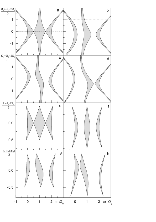
Figure 3: FIGURE 3.

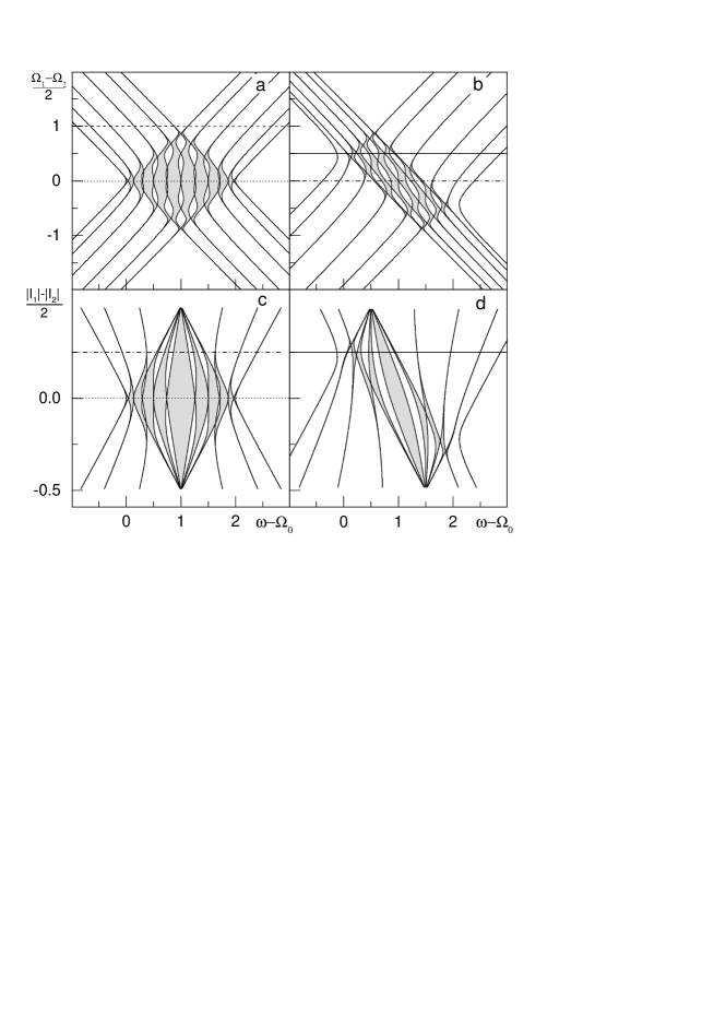
Figure 5: FIGURE 5.

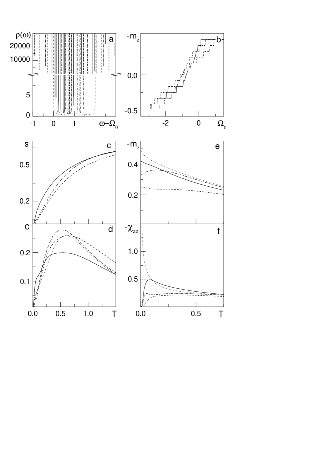
Figure 6: FIGURE 6.

Figure 8: FIGURE 8.

Figure 9: FIGURE 9.

Figure 10: FIGURE 10.

Figure 11: FIGURE 11.

Figure 12: FIGURE 12.

Figure 16: FIGURE 16.

Figure 17: FIGURE 17.

Figure 19: FIGURE 19.

References

[1]
E. Lieb, T. Schultz, and D. Mattis,
Ann. Phys. (N.Y.) 16, 407 (1961).
[2]
S. W. Lovesey,
J. Phys. C 21, 2805 (1988).
[3]
Ch. J. Lantwin and B. Stewart,
J. Phys. A 24, 699 (1991).
[4]
J. K. Freericks and L. M. Falicov,
Phys. Rev. B 41, 2163 (1990).
[5]
R. Łyżwa,
Physica A 192, 231 (1993).
[6]
P. Lloyd,
J. Phys. C 2, 1717 (1969).
[7]
W. John and J. Schreiber,
Phys. Status Solidi B 66, 193 (1974).
[8]
J. Richter,
Phys. Status Solidi B 87, K89 (1978).
[9]
H. Nishimori,
Phys. Lett. A 100, 239 (1984).
[10]
O. Derzhko and J. Richter,
Phys. Rev. B 55, 14298 (1997).
[11]
O. Derzhko and J. Richter,
Phys. Rev. B 59, 100 (1999).
[12]
V. M. Kontorovich and V. M. Tsukernik,
Sov. Phys. JETP 26, 687 (1968).
[13]
P. Pincus,
Solid State Commun. 9, 1971 (1971).
[14]
J. H. H. Perk, H. W. Capel, M. J. Zuilhof, and Th. J. Siskens,
Physica A 81, 319 (1975).
[15]
R. A. T. Lima and C. Tsallis,
Phys. Rev. B 27, 6896 (1983).
[16]
J. H. Taylor and G. Müller,
Physica A 130, 1 (1985)
(and references therein).
[17]
K. Okamoto and K. Yasumura,
J. Phys. Soc. Jpn. 59, 993 (1990)
(and references therein).
[18]
K. Okamoto,
J. Phys. Soc. Jpn. 59, 4286 (1990).
[19]
A. A. Zvyagin,
Phys. Lett. A 158, 333 (1991).
[20]
A. A. Zvyagin,
Fiz. Niz. Temp. (Kharkiv) 18, 788 (1992)
(in Russian).
[21]
K. Okamoto,
Solid State Commun. 83, 1039 (1992).
[22]
Y. Saika and K. Okamoto, cond-mat/9510114.
[23]
A. Fujii, cond-mat/9707137.
[24]
S. M. Bhattacharjee and S. Mukherji,
J. Phys. A 31, L695 (1998).
[25]
S. Sil,
J. Phys.: Condens. Matter 10, 8851 (1998).
[26]
L. L. Gonçalves and J. P. de Lima,
J. Magn. Magn. Mater. 140-144, 1606 (1995).
[29]
O. Derzhko, J. Richter, and O. Zaburannyi,
cond-mat/9909251, submitted to Phys. Lett. A.
[30]
Th. J. Siskens and P. Mazur,
Physica A 71, 560 (1974).
[31]
W. B. Jones and W. J. Thron,
Continued Fractions.
Analytic Theory and Applications
(Addison-Wesley Publishing Company,
London, Amsterdam, Don Mills, Ontario, Sydney, Tokyo,
1980).
[32]
R. Haydock, V. Heine, and M. J. Kelly,
J. Phys. C 5, 2845 (1972).
[33]
R. Haydock, V. Heine, and M. J. Kelly,
J. Phys. C 8, 2591 (1975).
[34]
R. Haydock,
Solid State Physics 35, 215 (1980).
[35]
M. J. Kelly,
Solid State Physics 35, 295 (1980).
[36]
A. S. Davydov,
Tjeorija tvjerdogo tjela
(Nauka, Moskwa, 1976) (in Russian).
[37]
M. Oshikawa, M. Yamanaka, and I. Affleck,
Phys. Rev. Lett. 78, 1984 (1997).
[38]
J. Villain, R. Bidaux, J.-P. Carton, and R. Conte,
J. Physique 41, 1263 (1980).
[39]
E. F. Shender,
Sov. Phys. JETP 56, 178 (1982).
[40]
J. Richter, S. E. Krüger, A. Voigt, and C. Gros,
Europhys. Lett. 28, 363 (1994).
[41]
M. Hase, I. Terasaki, and K. Uchinokura,
Phys. Rev. Lett. 70, 3651 (1993).
[42]
For a review on CuGeO3 see:
J. P. Boucher and L. P. Regnault,
J. Phys. I 6, 1939 (1996).
[43]
M. Hase, I. Terasaki, K. Uchinokura, M. Tokunaga, N. Miura,
and H. Obara,
Phys. Rev. B 48, 9616 (1993).
[44]
K. Hirota, M. Hase, J. Akimitsu, T. Masuda, K. Uchinokura,
and G. Shirane,
J. Phys. Soc. Jpn 67, 645 (1998).
[45]
V. N. Glazkov, A. I. Smirnov, O. A. Petrenko, D. MK. Paul,
A. G. Vetkin, and R. M. Eremina,
J. Phys.: Condens. Matter 10, 7879 (1998).
[46]
H. Fukuyama, T. Tanimoto, and M. Saito,
J. Phys. Soc. Jpn. 65, 1182 (1996).
[47]
H. Yoshioka and Y. Suzumura,
J. Phys. Soc. Jpn. 66, 3962 (1997).
[48]
M. Mostovoy, D. Khomskii, and J.Knoester,
Phys. Rev. B 58, 8190 (1998).
[49]
M. Fabrizio, R. Mélin, and J. Souletie,
cond-mat/9807093.
[50]Handbook of mathematical functions with formulas,
graphs and mathematical tables,
edited by M. Abramovitz and I. A. Stegun
(National Bureau of Standards, 1964).
[51]
M. C. Cross,
Phys. Rev. B 20, 4606 (1979).
[52]
J. Mertsching and H. J. Fishbeck,
Physica Status Solidi B 103, 783 (1981).
[53]
G. S. Uhrig, F. Schönfeld, and J. P. Boucher,
Europhys. Lett. 41, 431 (1998).
[54]
G. S. Uhrig, F. Schönfeld, M. Laukamp, and E. Dagotto,
Eur. Phys. J. B 7, 67 (1999).