On the evaluation of the specific heat and general off-diagonal n-point correlation functions within the loop algorithm

Abstract

We present an efficient way to compute diagonal and off-diagonal n-point correlation functions for quantum spin-systems within the loop algorithm. We show that the general rules for the evaluation of these correlation functions take an especially simple form within the framework of directed loops. These rules state that contributing loops have to close coherently. As an application we evaluate the specific heat for the case of spin chains and ladders.

I Introduction

Numerical investigations of strongly correlated electron systems [1] gained considerable importance in the last decade. The evaluation of non-diagonal correlation function and dynamical response function plays a major role in the context of correlated electron systems [1, 2]. On the other hand, there are only very few investigations of non-diagonal and/or higher-order correlation function in the context of quantum spin-systems. Indeed, it has been realized only recently, that non-diagonal correlation function might be calculated efficiently within the loop-algorithm [3]. The loop-algorithm [4] has established itself as the method of choice for quantum-Monte Carlo (MC) simulations of non-frustrated quantum spin systems.

The key observation here is the fact, that local updating dynamics in a MC simulation creates strongly correlated configurations for gapless quantum spin systems at low temperatures. Since the samples are then not statistically independent, the statistical error bars do decay only very slowly with the number of samples. One way to state this problem is to say, that the autocorrelation time $\tau_{auto}$ for the samples of spin-configurations created with the MC-walk increases (in generally exponentially) at low temperatures.

Most efficient MC procedures implement consequently global update dynamics. Examples of these procedures are the clusters algorithms [6]. Designed to circumvent the critical slowing down, these methods have been intensively used to study classical statistical systems near critical points, where the problem of large $\tau_{auto}$ is very severe.

The loop algorithm [4] can be considered as a generalization of classical clusters algorithms to quantum models. In fact, it gives a prescription on how global updates can be performed in quantum systems. As we will see this prescription lays on the geometric interpretation of the transformation from a quantum system to a statistical model of oriented loops. The MC procedure can be implemented then directly on the loops. It has the advantage that the updating dynamics defined on the loops generates statistically nearly independent configurations. The autocorrelation time is therefore about just MC step and the corresponding operators can be measured at every MC step avoiding both ’waiting times’ and substantial increments of the variance (statistical error bars).

In addition, a loop has another remarkable property; starting from an allowed spin configuration, constructing a loop and then flipping all spins in one loop (flipping the orientation of the loop) one obtains a new allowed configuration. This observation allows to compute the expectation value of operators not only in one configuration per MC step but in all configuration related to it by flipping any number of given loops. This procedure is usually called improved estimator [3].

The purpose of this work is to extend the algorithm to the computation of higher order (and non-diagonal) correlations functions. As we will see it involves dealing with two or more loop contributions. In particular we will focus on the specific heat $c_{V}$, which, in the past, has been considered a major challenge for Monte-Carlo simulations [7]. We will show, that the direct evaluation of the higher-order (non-diagonal) correlation functions contributing to $c_{V}$ allows for improved estimators and such to gain one order of magnitude in computational efficiency. The method that we presented is valid in any dimension.

II The Loop Algorithm

A nice review of the loop algorithm can be found in Ref. [5]. Here we start with a short introduction in order to introduce the notation used further on for the evaluation of higher-order correlation functions.

The loop algorithm is most easily understood in the checkerboard picture for a discrete number of Trotter slices $N_{T}$; the generalization to continuous Trotter time [8] is straightforward. This picture, which is based on the Suzuki-Trotter decomposition, describes in a graphical way how the interacting spin system wave function evolves in discrete imaginary time.

The Suzuki-Trotter formula [9] maps a quantum spin system in dimension $d$ onto a classical spin in dimension $d+1$. The partition function of the original quantum spin model is hereby written in terms of the trace of a product of transfer matrices defined in the classical model.

To illustrate the method we consider an inhomogeneous one-dimensional XXZ model $H=H_{1}+H_{2}$ on a bipartite chain of length $L$:

$\displaystyle H_{1}=\sum_{i=2m}H_{i},\qquad H_{2}=\sum_{j=2m+1}H_{j}$

$\displaystyle H_{i}=-\frac{J_{i}^{XY}}{2}\left(S_{i}^{+}S_{i+1}^{-}+S_{i}^{-}S_{i+1}^{+}\right)+J_{i}^{Z}S_{i}^{Z}S_{i+1}^{Z}~{},$where the sign of the term $\sim J_{i}^{XY}$ has been choose to be negative by an appropriate rotation of the spins on one of the two sublattices. This is always possible on a bipartite lattice and allows for positive transfer matrix elements (absence of the sign problem). The decomposition $H=H_{1}+H_{2}$ allows for the use of Totter-Suzuki formula [9] for the representation of the partition function $Z=\mbox{Tr}\left[\exp(-\frac{\beta}{N_{T}}H)\right]^{N_{T}}$,

$\displaystyle Z=\mbox{Tr}\prod_{n=1}^{N_{T}}\sum_{\alpha_{n}}\langle\phi_{\alpha_{n}}^{(n)}|\exp(-\Delta\tau H_{1})\exp(-\Delta\tau H_{2})|\phi_{\alpha_{n+1}}^{(n+1)}\rangle+O({\Delta\tau^{2}})~{},$where $\Delta\tau=\beta/N_{T}$. Here we have introduced representations of the unity operator $\sum_{\alpha_{n}}|\phi_{\alpha_{n}}^{(n)}\rangle\langle\phi_{\alpha_{n}}^{(n)}|$ in between any of the $N_{T}$ imaginary time slices.

Since $H_{1}$ and $H_{2}$ are sum of local operators that commute with each other, we may write the wave function as the product of the local basis in say z-component of spin, $|\phi_{\alpha_{n}}^{(n)}\rangle=\otimes_{i}|\sigma_{i}\rangle$, with $\sigma_{i}=\uparrow,\downarrow$.

In the checkerboard lattice the interaction between two consecutive pairs of spins is graphically denoted by shaded plaquettes (see Fig. 1). There are two spins interacting per plaquette so a 4x4 transfer matrix $T_{i}$ can be defined in each plaquette, which depends only one the coupling constants.

FIG. 1.: Illustration of a plaquette with a spin flip process which corresponds to the matrix element $\langle\uparrow\downarrow|\exp(-\Delta\tau H)|\downarrow\uparrow\rangle$ of the transfer matrix.

For the XXZ-model the transfer matrix $T_{i}$ is in the basis $\left(|\uparrow,\uparrow\rangle,|\uparrow,\downarrow\rangle,|\downarrow,\uparrow\rangle,|\downarrow,\downarrow\rangle\right)$:

$\displaystyle T_{i}=\mbox{e}^{{\Delta\tau J_{i}^{z}\over 4}}\left(\begin{array}[]{cccc}\exp(-\frac{\Delta\tau J^{Z}_{i}}{2})&0&0&0\\ 0&\cosh(\frac{\Delta\tau J^{XY}_{i}}{2})&\sinh(\frac{\Delta\tau J^{XY}_{i}}{2})&0\\ 0&\sinh(\frac{\Delta\tau J^{XY}_{i}}{2})&\cosh(\frac{\Delta\tau J^{XY}_{i}}{2})&0\\ 0&0&0&\exp(-\frac{\Delta\tau J^{Z}_{i}}{2})\end{array}\right)~{}.$The partition function $Z$ is then, up to terms order $O(\Delta\tau^{2})$, the trace of a product of transfer matrices:

$\displaystyle Z=\mbox{Tr}\left[\exp(-\beta H)\right]=\mbox{Tr}\prod_{n=1}^{N_{T}}\left(\bigotimes_{i=2m}T_{i}\right)\left(\bigotimes_{j=2m+1}T_{j}\right)~{}.$As a next step beyond this standard representation of $d$-dimensional quantum models in terms of classical statistical systems [10] we expanded the transfer matrices $T_{i}=\sum_{\gamma}p_{i}^{(\gamma)}M^{(\gamma)}$ in terms of certain matrices $M^{(\gamma)}$ such that the weight $p^{(\gamma)}_{i}\geq 0$ are non-negative. This is, in general, not possible for all models. For the XXZ with $J^{XY}_{i}\geq J_{i}^{Z}$ we can choose:

$\displaystyle M^{(1)}=\left(\begin{array}[]{cccc}1&0&0&0\\ 0&1&0&0\\ 0&0&1&0\\ 0&0&0&1\end{array}\right),\quad M^{(2)}=\left(\begin{array}[]{cccc}1&0&0&0\\ 0&0&1&0\\ 0&1&0&0\\ 0&0&0&1\end{array}\right),\quad M^{(3)}=\left(\begin{array}[]{cccc}0&0&0&0\\ 0&1&1&0\\ 0&1&1&0\\ 0&0&0&0\end{array}\right)~{},$where $p_{i}^{(1)}=\frac{1}{2}(\exp(-\Delta\tau J^{z}_{i}/2)+\exp(-\Delta\tau J^{XY}_{i}/2))\exp(\Delta\tau J^{Z}_{i}/4)$, $p_{i}^{(2)}=\frac{1}{2}(\exp(-\Delta\tau J^{z}_{i}/2)-\exp(-\Delta\tau J^{XY}_{i}/2))\exp(\Delta\tau J^{Z}_{i}/4)$ and $p_{i}^{(3)}=\frac{1}{2}(-\exp(-\Delta\tau J^{z}_{i}/2)+\exp(\Delta\tau J^{XY}_{i}/2))\exp(\Delta\tau J^{Z}_{i}/4)$. We then obtain for the partition function

$$Z=\mbox{Tr}\prod_{n=1}^{N_{T}}\bigotimes_{i=2m}\left(\sum_{\gamma}p_{i}^{(\gamma)}M^{(\gamma)}\right)\bigotimes_{j=2m+1}\left(\sum_{\gamma}p_{j}^{(\gamma)}M^{(\gamma)}\right)$$ (1)

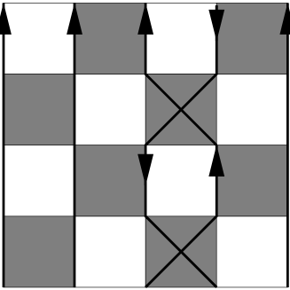
FIG. 2.: Evolution of worldlines of up and down spins in imaginary time. Periodic boundary conditions are assumed in both space and imaginary time. Note that we define worldlines for both up- and down-spins, which differ by the direction in imaginary time.

Eq. (1) can be interpreted in a geometrical way (see Fig. 2). In the checkerboard picture the $M^{(\gamma)}$ matrices can be understood as different ways in which the worldlines can be broken in every plaquette and are usually called breakups. By taking one breakup per every plaquette we force the worldlines into closed paths which we call directed loops (see Fig. 3). A directed loop therefore follows the worldline of an up-spin when it evolves in positive Trotter-time direction and the world-line of a down-spin when it evolves in negative Trotter-time direction.

In Fig. 3 we show the graphic representation of the breakups $M^{(\gamma)}$. The lines now represent the directed loop segments.

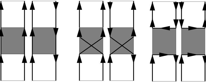
FIG. 3.: Illustration of loop breakups, the directed lines represent the loop segments. From left to right the vertical ($M^{(1)}$), diagonal ($M^{(2)}$) and the horizontal breakup ($M^{(3)}$) are shown.

Eq. (1) states that the partition function can be obtained as a sum over all breakups. As a sum over all breakups is equivalent to a sum over all loop configurations $\{l\}$ we may rewrite Eq. (1) as

$$Z=\sum_{\{l\}}\rho(\{l\})\ \mbox{Tr}\prod_{n=1}^{N_{T}}\bigotimes_{i=2m}M^{(\gamma_{i})}\bigotimes_{j=2m+1}M^{(\gamma_{j})}~{},$$ (2)

where $\rho(\{l\})=\prod_{i}p_{i}^{(\gamma_{i})}\prod_{j}p_{j}^{(\gamma_{j})}$. Eq. (2) leads to a very efficient MC-algorithm [4]: (a) Choose loop-breakups $M^{(\gamma_{i})}$ with probabilities $p_{i}^{(\gamma_{i})}$. (b) Construct the loop configuration $\{l\}$ and flip all loops with probability $1/2$. (c) Measure any desired operator in all $2^{N_{L}(\{l\})}$ spin configurations reachable with independent loop flips (improved estimators), where $N_{L}(\{l\})$ is the number of loops in the loop configuration $\{l\}$.

For later use we rewrite Eq. (2) in a form of traces over individual loops. Noting that vertical and diagonal loop segments do not change the spin-direction (see Fig. 3), we may associate the $2\times 2$ identity matrix $\sigma^{0}=\left(\begin{array}[]{cc}1&0\\ 0&1\end{array}\right)$ with vertical and diagonal loop segments. As horizontal loop segments do change the spin-direction, we associate the Pauli-matrix $\sigma^{x}=\left(\begin{array}[]{cc}0&1\\ 1&0\end{array}\right)$ with them. We then may rewrite Eq. (2) as

$$Z=\sum_{\{l\}}\rho(\{l\})\,\prod_{l\in\{l\}}\mbox{Tr}_{l}\prod_{\mu}\sigma^{\gamma_{\mu}}~{},$$ (3)

where $\mu$ is an index running over loop $l$ and $\gamma_{\mu}=0,x$. $\mbox{Tr}_{l}$ denotes the trace over loop $l$. Since $\mbox{Tr}_{l}\prod_{\mu}\sigma^{\gamma_{\mu}}=2$, Eq. (3) is equivalent to a statistical mechanical model of oriented loops, $Z=\sum_{\{l\}}\rho(\{l\})\ 2^{N_{L}(\{l\})}$.

III Correlation functions, improved estimators

The expectation value of an operator ${\cal O}$ is

$$\langle{\cal O}\rangle=\mbox{Tr}({\cal O}\exp(-\beta H))=\sum_{\alpha,\beta}\langle\phi_{\alpha}|{\cal O}|\phi_{\beta}\rangle\langle\phi_{\beta}|\exp(-\beta H)|\phi_{\alpha}\rangle$$ (4)

If ${\cal O}$ is diagonal in the basis $\{|\phi_{\alpha}\rangle\}$ then this procedure is straightforward. The updating procedure generates a sequence of configurations $c_{i_{MC}}$ ($i_{MC}=1\dots N_{MC}$), according with the distribution function of the system. In these configurations ${\cal O}$ takes a well defined value ${\cal O}(c_{i_{MC}})$, therefore:

$$\langle{\cal O}\rangle=\frac{1}{N_{MC}}\sum_{i_{MC}}{\cal O}(c_{i_{MC}})~{}.$$ (5)

The loop algorithm allows to measure an operator not only in $c_{i_{MC}}$ but in all configurations related by loop flippings. We illustrate the use of these improved estimators by computing ${\cal O}=S^{z}_{\bf x}S^{z}_{\bf y}$ (here indices $\bf x$ and $\bf y$ label both space and Trotter time (see Fig. 4). When $\bf x$ and $\bf y$ belong to different loops the orientation can be changed independently and the total contribution cancels. By the contrary when $\bf x$ and $\bf y$ are on the same loop the orientations of the loop in both sites are linked and these terms contribute for the two possible orientations of the loop.

FIG. 4.: Summing over all possible loop orientations, the two-loop contributions cancel each other for $S^{z}_{\bf x}S^{z}_{\bf y}$. Only when the two spin-operators act on the same loop we get a non-vanishing contribution.

We will consider now the problem of non diagonal operators. The expectation value of a non diagonal operator ${\cal O^{\prime}}$ in the loop picture is, see Eq. (2):

$$\langle{\cal O^{\prime}}\rangle=\sum_{\{l\}}\rho(\{l\})\,\mbox{Tr}{\cal T}\left({\cal O^{\prime}}\prod_{n=1}^{N_{T}}\bigotimes_{i}M^{(\gamma_{i})}\bigotimes_{j}M^{(\gamma_{j})}\right)~{},$$ (6)

where ${\cal T}()$ means proper imaginary time ordering. Let us take as an example the two-point correlator ${\cal O^{\prime}}=S^{+}_{\bf x}S^{-}_{\bf y}$,

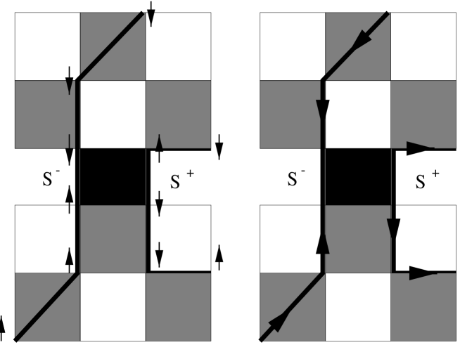
FIG. 5.: The action of $S^{-}_{\bf x}S^{+}_{\bf y}$ can be represented as the insertion of a new kind of plaquette, here depicted in black, which acts on two loop segments. This operator flips the spins and changes therefore the orientation of the two loops for the remaining segments. Left-picture: The arrows denote the spin-direction. Right-picture: The arrows denote the direction of the loops.

Graphically the evaluation of an operator can be interpreted on the checkerboard framework as the insertion of a new kind of plaquette. In Fig. 5 we show the action of that operator in the checkerboard picture. We note that an off-diagonal operator in general reverses the direction of one or more loops. The loop configurations generated by the MC updating-procedure does, on the other hand, only generate loops with well defined loop orientations. Nevertheless there is a close connection between these two types of configurations which is easy to understand in graphical terms.

FIG. 6.: If $S^{+}_{\bf x}$ and $S^{-}_{\bf y}$ operate on different loops none of them can be closed consistently in terms of loop orientation, represented here by arrows. When both operators act on the same loop that configuration contributes to $\langle S^{+}_{\bf x}S^{-}_{\bf y}\rangle$.

In Fig. 5 it is shown how the flipping of one spin ’propagates’ through the loop, changing the orientation of the loop from that point. Thinking in terms of oriented loops it is obvious that with only one of these flipping processes ($S_{x}^{+}$ or $S_{y}^{-}$) per loop, it is not possible to close the loop consistently. To reestablish the original loop orientation it is necessary to have an even number of properly ordered $S^{-}$ or $S^{+}$ operators on the same loop to close it consistently in terms of loop orientation variables. A loop which is not properly closed does not contribute to $\langle{\cal O^{\prime}}\rangle$. Then we can establish that for a two-point correlation function we only obtain a contribution when $x$ and $y$ belong to the same loop (see Fig. 6). Eq. (4) could suggest that measurements of non diagonal operators consume more computing time than diagonal operators, but using this graphical picture we note that both computations can be implemented in an equivalent way.

These ideas can be justified in formal terms using Eq. (3) and Eq. (6). The $S^{+}_{\bf x}$ and $S^{-}_{\bf y}$ operators are placed in between of two $\sigma^{\gamma}$ matrices belonging to neighboring plaquettes and traces can be taken again independently in each loop. We define the $2\times 2$ matrices $\sigma^{+}=\left(\begin{array}[]{cc}0&1\\ 0&0\end{array}\right)$ and $\sigma^{-}=\left(\begin{array}[]{cc}0&0\\ 1&0\end{array}\right)$. For positive loop-direction (with respect to the Trotter direction) $S^{+}$ is equivalent to $\sigma^{+}$, for a directed loop segment with negative loop-direction $S^{+}$ is equivalent to $\sigma^{-}$. For $S^{-}$ it is just the other way round. The loop direction of relevance here is the one before the insertion of either a $S^{+}$ or a $S^{-}$ operator.

We start considering contributions to $\langle S^{+}_{\bf x}S^{-}_{\bf y}\rangle$ where the loop-direction at site $\bf x$ is up and down at site $\bf y$ (see Fig. 6). The expectation value of the non-diagonal operator $S^{+}_{\bf x}S^{-}_{\bf y}$ then becomes (compare Eq. (3))

$$\langle S^{+}_{\bf x}S^{-}_{\bf y}\rangle\rightarrow{1\over Z}\sum_{\{l\}}\rho(\{l\})\,{\cal T}\left(\sigma_{\bf x}^{+}\sigma_{\bf y}^{+}\prod_{l\in\{l\}}\mbox{Tr}_{l}\prod_{\mu}\sigma^{\gamma_{\mu}}\right)~{}.$$ (7)

Here ${\cal T}$ means proper time and space ordering. When $\sigma^{+}_{\bf x}$ and $\sigma^{+}_{\bf y}$ are placed in different loops, the traces taken in these two loops cancel. If they are in the same loop the trace taken in that loop equals 1 (and not 2), independently of the spin-configuration. We will prove this last point now. We start by writing the partial trace of the loop containing $\sigma^{+}_{\bf x}$ and $\sigma^{-}_{\bf y}$ as

$\displaystyle T^{(++)}=\mbox{Tr}_{l}\,\sigma_{\bf x}^{+}\left(\sigma^{x}\right)^{z_{1}}\sigma_{\bf y}^{+}\left(\sigma^{x}\right)^{z_{2}}~{},$where we neglected the $\sigma^{0}$ matrices, as they are just the identity matrices. We note that $z_{1}+z_{2}$ is even since $\left(\sigma^{x}\right)^{2}=\sigma^{0}$ and because we are considering a loop which did contribute to the partition function $Z$ before the $S_{\bf x}^{+}S_{\bf y}^{-}$ operators were inserted. The $\sigma^{x}$ matrix corresponds to a horizontal loop segment and such to a change in loop direction. $z_{1}$ needs therefore to be odd (and therefore also $z_{2}$), since one needs an odd number of directional inversions to arrive to a negative loop direction at site $\bf y$, starting from a positive direction at site $\bf x$. We may therefore rewrite $T^{(++)}$ (using again $\left(\sigma^{x}\right)^{2}=\sigma^{0}$) as

$\displaystyle T^{(++)}=\mbox{Tr}_{l}\,\sigma_{\bf x}^{+}\sigma^{x}\sigma_{\bf y}^{+}\sigma^{x}\equiv 1~{},$as one can easily evaluate. Similarly one can consider the case when the initial loop directions are both positive at sites $\bf x$ and $\bf y$. The expectation value of the non-diagonal operator $S^{+}_{\bf x}S^{-}_{\bf y}$ becomes then in this case

$$\langle S^{+}_{\bf x}S^{-}_{\bf y}\rangle\rightarrow{1\over Z}\sum_{\{l\}}\rho(\{l\})\,{\cal T}\left(\sigma_{\bf x}^{+}\sigma_{\bf y}^{-}\prod_{l\in\{l\}}\mbox{Tr}_{l}\prod_{\mu}\sigma^{\gamma_{\mu}}\right)~{}.$$ (8)

The corresponding one-loop contributions then have the form

$\displaystyle T^{(+-)}=\mbox{Tr}_{l}\,\sigma_{\bf x}^{+}\left(\sigma^{x}\right)^{z_{1}}\sigma_{\bf y}^{-}\left(\sigma^{x}\right)^{z_{2}}=\mbox{Tr}_{l}\,\sigma_{\bf x}^{+}\sigma_{\bf y}^{-}\equiv 1~{},$since both $z_{1}$ and $z_{2}$ have to be even in this case. Similarly one can consider the two remaining cases of loop directions down/up and down/down at the sites $\bf x$ and $\bf y$. It is worthwhile noting, that one easily proves along these lines the expected result $\langle S^{+}_{\bf x}S^{+}_{\bf y}\rangle=0$.

IV General case n-point correlation functions

In the last section we have shown how the loop orientation is the fundamental variable to deal with the computation of correlation functions using improved estimators. In fact the problem of n-point correlation functions can also be reduced to the study of how the loop orientation is changed by the action of some operators.

FIG. 7.: Schematic example of two disconnected one-loop contributions to $\langle{\cal O}^{\prime\prime}\rangle$. The dotted line in between two operators illustrates the case of two operators at the same Trotter time.

We illustrate the case of two-loop terms for the four-point correlation function ${\cal O}^{\prime\prime}=S_{\bf x}^{+}S_{\bf y}^{-}S_{{\bf x}^{\prime}}^{+}S_{{\bf y}^{\prime}}^{-}$. Here we consider the case relevant for the specific heat were $({\bf x},{\bf y})$ and $({\bf x}^{\prime},{\bf y}^{\prime})$ are pairs of real-space nearest neighbor (n.n.) sites at the same Trotter time. This operator can generate several different kinds of contributions. The first one is the case of two disconnected one-loop contributions (see Fig. 7). This is the case if $S_{\bf x}^{+}$ and $S_{\bf y}^{-}$ act in one loop and $S_{{\bf x}^{\prime}}^{+}$ and $S_{{\bf y}^{\prime}}^{-}$ in a second loop. A second contribution arises if $S_{\bf x}^{+}$ and $S_{{\bf y}^{\prime}}^{-}$ act in one loop and $S_{\bf y}^{-}$ and $S_{{\bf x}^{\prime}}^{+}$ in a second loop (see Fig. 8). We call this contribution a connected two-loop contribution. A third contribution arises when all four sites act on the same loop.

FIG. 8.: Schematic example of connected two-loop contribution. Two n.n. operators at the same Trotter time are connected with a dotted line.

The evaluation of a single off-diagonal four-point operator ${\cal O}^{\prime\prime}$ does not pose a problem within the loop algorithm. For the case of interest, the specific heat a few additional points need to be kept in mind. The specific heat $c_{V}$ is given by

$$c_{V}=\frac{\beta^{2}}{L\,N_{T}^{2}}\left[\sum_{{\bf x},{\bf x}^{\prime}}\langle\,({\bf S}_{\bf x}\cdot{\bf S}_{\bf y})({\bf S}_{{\bf x}^{\prime}}\cdot{\bf S}_{{\bf y}^{\prime}})\,\rangle-\left(\sum_{\bf x}\langle{\bf S}_{\bf x}\cdot{\bf S}_{\bf y}\rangle\right)^{2}\right]~{},$$ (9)

where, again, $({\bf x},{\bf y})$ and $({\bf x}^{\prime},{\bf y}^{\prime})$ are pairs of (real-space) n.n. sites on the Trotter lattice. The first term of Eq. (9) is a local energy-energy correlation function. When, $\bf x$ and $\bf y$ belong to a loop and ${\bf x}^{\prime}$ and ${\bf y}^{\prime}$ to another, we generate two-loop disconnected terms (as the one illustrated in Fig. 7) that can be computed from the expectation value of the internal energy, the second term of specific heat. The energy in a given MC-configuration, $E_{i_{MC}}$, can be written as a sum of the energy in the $N_{L}(i_{MC})$ loops in this MC-configuration:

$\displaystyle E_{i_{MC}}=\sum_{l=1}^{N_{L}(i_{MC})}E_{i_{MC}}^{l}~{}.$

With this definition we obtain

$\displaystyle c_{V}^{(ind)}={1\over N_{MC}}\sum_{i_{MC}}\sum_{l\neq k}E_{i_{MC}}^{l}E_{i_{MC}}^{k}={1\over N_{MC}}\sum_{i_{MC}}\left[\left(\sum_{l}E_{i_{MC}}^{l}\right)^{2}-\sum_{l}\left(E_{i_{MC}}^{l}\right)^{2}\right]~{},$where $c_{V}=c_{V}^{(conn)}+c_{V}^{(ind)}$. For the evaluation of the connected term $c_{V}^{(conn)}$ one has to evaluate the off-site terms, $c_{V}^{(off)}$, where the pairs $({\bf x},{\bf y})$ and $({\bf x}^{\prime},{\bf y}^{\prime})$ are disjunct, separately from the on-site terms, $c_{V}^{(on)}$, where they are not disjunct: $c_{V}^{(conn)}=c_{V}^{(off)}+c_{V}^{(on)}$. By spin-algebra the on-site terms reduce to general two-point correlation functions. The (connected) off-site contributions fall in three categories, depending on the number $S^{z}$ operators involved (four, two or zero). The contributions with four $S^{z}$ operators have one and two loop contributions. A connected term with two $S^{z}$ operators has no two-loop contribution. Every correlation with two $S^{z}$ operators has the form $S^{z}_{\bf x}S^{z}_{\bf y}S^{+}_{{\bf x}^{\prime}}S^{-}_{{\bf y}^{\prime}}$. If the indices ${\bf x}$ and ${\bf y}$ are not in the same loop the two $S^{z}$ operators act in different loops and their traces cancel for the reason explained in section III. The same reasoning is valid for ${\bf x}^{\prime}$ and ${\bf y}^{\prime}$ with the operators $S^{+}$ and $S^{-}$. Finally, terms with no $S^{z}$ operators can have two loop contributions (see Fig. 8) and also one-loop contributions when the $S^{+}$ and $S^{-}$ are properly ordered along the loop to close the loop coherently in terms of loop orientation. On the left of Fig. 9 we see that an arbitrary insertion of the operators $S^{+}$ and $S^{-}$ can produce a conflict on the orientation of the loop. Technically, the value of the trace taken along the loop will depend on the structure of the correlator. This structure determines the order of the insertion of the $\sigma^{+}$ and $\sigma^{-}$ matrices. For example the trace along the loop on the left of Fig. 9 is:

$\displaystyle\mbox{Tr}(\sigma^{-}_{\bf x}\sigma^{x}\sigma^{-}_{{\bf x}^{\prime}}\sigma^{-}_{\bf y}\sigma^{x}\sigma^{+}_{{\bf y}^{\prime}})=0~{}.$For the loop on the right of Fig. 9 it is:

$\displaystyle\mbox{Tr}(\sigma^{-}_{\bf x}\sigma^{x}\sigma^{-}_{\bf y}\sigma^{+}_{{\bf x}^{\prime}}\sigma^{x}\sigma^{+}_{{\bf y}^{\prime}})=1~{}.$

FIG. 9.: On the left we show an example of non-contributing configuration to the specific heat. The loop orientation is ill defined and therefore this configuration does not contribute. On the right we see a contributing one-loop configuration.

It is possible to evaluate certain off-diagonal operators $\cal O$ by an alternative method. The condition is, that the operator can be expressed by a sum of local operators which do involve the same pairs of sites $\langle l,l^{\prime}\rangle$ as the Hamilton-operator $H=\sum_{\langle l,l^{\prime}\rangle}H_{l,l^{\prime}}$: ${\cal O}=\sum_{\langle l,l^{\prime}\rangle}{\cal O}_{l,l^{\prime}}$. It is then possible to compute $\langle\cal O\rangle$ by a reweighting method. The idea is to extend the plaquette of the checkerboard representation by new internal degrees of freedom, $\sum_{\beta}|\phi_{\beta}\rangle\langle\phi_{\beta}|$ (see Fig. 10). The reweighted matrix element of $\langle{\cal O}_{x,x^{\prime}}\rangle$ is then

$${\cal O}_{\alpha_{n},\alpha_{n+1}}^{(n)}(x,x^{\prime})=\sum_{\beta}\,{\langle\phi_{\alpha_{n}}^{(n)}|{\cal O}_{x,x^{\prime}}|\phi_{\beta}\rangle\,\langle\phi_{\beta}|\exp(-\Delta\tau H_{x,x^{\prime}})|\phi_{\alpha_{n+1}}^{(n+1)}\rangle\over\langle\phi_{\alpha_{n}}^{(n)}|\exp(-\Delta\tau H_{x,x^{\prime}})|\phi_{\alpha_{n+1}}^{(n+1)}\rangle}~{},$$ (10)

where $x$ and $x^{\prime}$ denote combined space-time indices. For a given spin-configuration $c_{i_{MC}}=\{\phi_{\alpha_{n}}^{(n)}|(n=1,\dots,N_{T})\}$ the off-diagonal expectation value of ${\cal O}(c_{i_{MC}})$ is ${\cal O}(c_{i_{MC}})=1/N_{T}\sum_{\langle x,x^{\prime}\rangle,(n)}{\cal O}_{\alpha_{n},\alpha_{n}+1}^{(n)}(x,x^{\prime})$ and $\langle{\cal O}\rangle=1/N_{MC}\sum_{i_{MC}}{\cal O}(c_{i_{MC}})$ (see Eq. (5)).

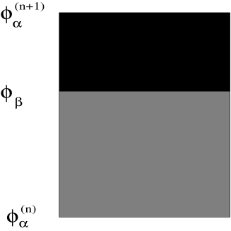
FIG. 10.: New structure of the plaquette in the reweighting method. The grey plaquette is the conventional plaquette where the evolution in imaginary time takes place, the black plaquette represents the operator $\cal{O}$ on the basis of $\sigma_{z}$. The product of the two matrices generates a new composite plaquette where the new weight is defined.

The reweighting method may also be applied to specific heat, which is the sum of products of local operators.

From the point of view of the complexity of the algorithm, measuring four-point correlation functions requires more computing time than two-point correlation functions. For the latter is only necessary to know whether or not two sites are in the same loop. This information can be obtained at the same time the loop is constructed and consequently the computing time remains proportional to $LN_{T}$. For n-point correlation functions the situation is more complex. In this case, there are contributions involving two or more loops and at the same time non-diagonal operators give different contributions depending on how they are ordered on the loop. In practice this depends on the shape of the loops in each configuration. A rigorous study of the performance of the method must include an analysis of the behavior of the statistical errors as a function of the temperature, size, number and type of operator involved in the correlation functions and the details of the Hamiltonian. This detailed analysis of technical aspects of n-point correlations will be presented elsewhere.

V Results

As an application of the rules explained in this paper we have computed the specific heat for a Heisenberg chain and for a ladder with $J_{\perp}=0.5J$ (which corresponds to the ratio for the ladder-compound Sr₁₄Cu₂₄O₄₁ [12]).

FIG. 11.: Specific heat for the Heisenberg model in the 8-site chain with $J=2$, as a function of temperature in units of $J$. The two sets of data correspond to the QMC simulations with improved estimators (open squares) and with the reweighting method (filled triangles), for the same number of QMC steps. The solid line is the exact diagonalization data.

In Fig. 11 we compare exact diagonalization results with the results using the method described above and the reweighting method for the same number of MC steps. The error bars in these two methods are also compared. For the lowest temperature the error bar with improved estimators are 6 times smaller. Taking into account that error bars decay as $\frac{1}{\sqrt{N_{MC}}}$ we expect that without using improved estimators 36 times more MC steps are necessary to get equal size error bars. The statistical errors are amplified by the factor $\beta^{2}$. This factor and the substraction of similarly large numbers lead to large error bars at low temperatures.

In the Fig. 12 we present results for the specific heat of a 100-site Heisenberg chain. To reproduce the linear regime at low temperatures it is necessary to perform a careful extrapolation to $\Delta\tau\rightarrow 0$ taking half a million of MC steps for each $\Delta\tau$ values and 10 different $N_{T}$ values ranging from 20 to 200.

FIG. 12.: Specific heat for a 100 sites Heisenberg with J=2.0 chain using improved estimators, as a function of temperature, in units of $J$. The error-bars are smaller than the symbol sizes. The solid line is the exact Bethe-Ansatz result for the infinite-chain [11].

In Fig. 13 we present results for the two-leg ladder of $2\times 201$ sites with twisted boundary conditions (i.e. for $J_{\perp}=0$ this system corresponds to a L=402-site Heisenberg chain).

FIG. 13.: Specific heat for the $2\times 201$ ladder with twisted boundary conditions as a function of temperature in units of $J$. The values of the couplings are $J=1.0$ and $J_{\perp}=0.5J$.

VI Conclusions

We have presented detailed rules on how to evaluate general, off-diagonal n-point Greens functions within the loop algorithm. These rules have a very simple interpretation in the picture of oriented loops. They state that the loop-orientation has to close coherently whenever a certain number of non-diagonal operators are inserted. We have shown how to apply these rules to the case of the specific heat and presented results for the 1D-Heisenberg model and a ladder system.

VII Acknowledgments

We would like to acknowledge discussions with Matthias Troyer, Naoki Kawashima and Andreas Klümper and the support of the German Science Foundation. We acknowledge the hospitality of the ITP in Santa Barbara. This research was supported by the National Science Foundation under Grant No. PHY94-07194.

REFERENCES

• [1] See for instance E. Dagotto, Rev. Mod. Phys. 66, 763 (1994) and references therein.
• [2] J.E. Hirsch and R.M. Feye, Phys. Rev. Lett. 56, 2521 (1986).
• [3] R. Brower, S. Chandrasekaran, U.-J. Wiese, Physica A 261, 520 (1998).
• [4] H.G. Evertz, G. Lana and M. Marcu, Phys. Rev. Lett. 70, 875 (1993).
• [5] H.G. Evertz in “Numerical Methods for Lattice Quantum Many-Body Problems.” ed. D.J. Scalapino, Addison Wesley Longman, Frontiers in Physics.
• [6] R.H. Swendsen, J.S. Wang, Phys. Rev. Lett. 58,86 (1987); U. Wolff, Phys. Rev. Lett. 62, 361 (1989).
• [7] C. Huscroft, R. Gass, M. Jarrell, Cond-mat 9906155; R. Fey and R. Scalettar, Phys. Rev. B 36, 3833 (1987).
• [8] B.B. Beard and U.-J. Wiese, Phys. Rev. Lett. 77, 5130 (1996).
• [9] H.F. Trotter, Proc. Am. Math. Soc. 10, 545 (1959); M. Suzuki, Prog. Theor. Phys. 56, 1454 (1976).
• [10] B.B. Beard and U.-J. Wiese, Phys. Rev. Lett. 77, 5130 (1996).
• [11] A. Kümper and D.C. Johnston, connd-mat/0002140; A. Klümper, personal communication.
• [12] E. Dagotto and T.M. Rice, Science 271, 618 (1996); E. Dagotto, cond-mat/9908250.