Statistical Physics of Structural Glasses

Abstract

This paper gives an introduction and brief overview of some of our recent work on the equilibrium thermodynamics of glasses. We have focused onto first principle computations in simple fragile glasses, starting from the two body interatomic potential. A replica formulation translates this problem into that of a gas of interacting molecules, each molecule being built of $m$ atoms, and having a gyration radius (related to the cage size) which vanishes at zero temperature. We use a small cage expansion, valid at low temperatures, which allows to compute the cage size, the specific heat (which follows the Dulong and Petit law), and the configurational entropy. The no-replica interpretation of the computations is also briefly described. The results, particularly those concerning the Kauzmann tempaerature and the configurational entropy, are compared to recent numerical simulations.

1 Introduction

While the experimental and phenomenological knowledge on glasses has improved a lot in the last decades[2], the progress on a first principle, statistical mechanical study of the glass phase has turned out to be much more difficult.

Take any elementary textbook on solid state physics. It deals with a special class of solid state, the crystalline state, and usually avoids to elaborate on the possibility of amorphous solid states. The reason is very simple: there is no theory of amorphous solid states. Schematically, the first elementary steps of the theory of crystals are the following. One computes the ground state energy of all the crystalline structures. The small vibrations around these structures are easily handled, either using the simple Einstein approximation of independent atoms in harmonic traps, or computing the phonon dispersion relations and going to the Debye theory. Then one can study the one electron problem and compute the band structure. The basic thermodynamic properties are already well reproduced by these elementary computations. Anharmonic vibrations, electron-phonon and electron-electron interactions can then be added to these basic building blocks.

Until very recently, none of the above computations, even in the simplest-minded approximation, could be done in the case of the glass state. The reason is obvious: all of them are made possible in crystals by the existence of the symmetry group. The absence of such a symmetry, which is a defining property of the glass state, forbids the use of all the solid state techniques. If one takes a snapshot of a glass state, an instantaneous configuration of atoms, it looks more like a liquid configuration. In fact the techniques which we shall use are often borrowed from the theory of the liquid state. But while the liquid phase is ergodic (which means that the probability distribution of positions is translationally invariant), the glass phase is not. The problem is to describe a non-ergodic phase without a symmetry: an amorphous solid state.

The work which we report on here has been elaborated during the last year and aims at building the first steps of a first principle theory of glasses. The fact that this is being made possible now is not fortuitous, but rather results from a conjunction of several sets of ideas, and the general progress of the last two decades on the theory of amorphous systems.

The oldest ingredients are the phenomenological ideas, originating in the work of Kauzmann [3], and developed among others by by Adam, Gibbs and Di-Marzio [4], which identify the glass transition as a ‘bona fide’ thermodynamic transition blurred by some dynamical effects. As we shall discuss below, in this scenario the transition is associated with an ‘entropy crisis’, namely the vanishing of the configurational entropy of the thermodynamically relevant glass states.

A very different, and more indirect, route, was the study of spin glasses. These are also systems which freeze into amorphous solid states, but one of their constitutive properties is very different from the glasses we are interested in here: there exists in spin glasses some ‘quenched disorder’: the exchange-interaction coupling constants between the spin degrees of freedom are quenched (i.e. time independent on all experimental time scales) random variables[5]. Anyhow, a few years after the replica symmetry breaking (RSB) solution of the mean field theory of spin glasses [6], it was realized that there exists another category of mean-field spin glasses where the transition is due to an entropy crisis [7]. These are now called discontinuous spin glasses because their phase transition, although it is of second order in the Ehrenfest sense, has a discontinuous order parameter, as first shown in [8]. Another name often found in the literature is ‘one step RSB’ spin glasses, because of the special pattern of symmetry breaking involved in their solution. The simplest example of these is the Random Energy Model [7], but many other such discontinuous spin glasses were found subsequently, involving multispin interactions [8, 9, 10].

The analogy between the phase transition of discontinuous spin glasses and the thermodynamic glass transition was first noticed by Kirkpatrick, Thirumalai and Wolynes in a series of inspired papers of the mid-eighties [9]. While some of the basic ideas of the present development were around at that time, there still missed a few crucial ingredients. On one hand one needed to get more confidence that this analogy was not just fortuitous. The big obstacle was the existence (in spin glasses) versus the absence (in structural glasses) of quenched disorder. The discovery of discontinuous spin glasses without any quenched disorder [11, 12, 13] provided an important new piece of information: contrarily to what had been believed for long, quenched disorder is not necessary for the existence of a spin glass phase (but frustration is). A second confirmation came very recently from the developments on out of equilibrium dynamics of the glass phase. Initiated by the exact solution of the dynamics in a discontinuous spin glass by Cugliandolo and Kurchan [14], this line of research has made a lot of progress in the last few years. It has become clear that, in realistic systems with short range interactions, the pattern of replica symmetry breaking can be deduced from the measurements of the violation of the fluctuation dissipation theorem [15]. Although these difficult measurements are not yet available, numerical simulations performed on different types of glass forming systems have provided an independent and spectacular confirmation of their ‘one step rsb’ structure [16, 17, 18] on the (short) time scales which are accessible. The theory was then facing the big challenge: understanding what this replica symmetry breaking could mean, in systems void of quenched disorder, in which there is thus no a priori reason to introduce replicas. The recent progress has brought the answer to this question and turned it into a computational method, allowing for a first principle computation of the equilibrium thermodynamics of glasses [19, 20, 21, 22, 23, 24].

In the context of glasses, the words ‘equilibrium thermodynamics’ call for some comments. First, it is not obvious whether the glass phase is an equilibrium phase of matter. It might be a metastable phase, reachable only by some fast enough quench, while the ‘true equilibrium’ phase would always be crystalline. The answer depends on the interaction potential. Numerically it is known that the frustration induced by considering for instance binary mixtures of soft spheres of different radii strongly inhibits crystallisation. But what is the true equilibrium state is unknown, and not very relevant. One can study crystals without having proven that they are stable phases of matter (by the way, simply proving that the fcc-hcp is the densest packing of hard spheres in 3 dimensions, a simple zero temperature statement, has resisted the efforts of scientists for centuries [25]), and one can study the properties of diamond, even though it is notoriously unstable. The point is to have reproducible properties, which is certainly the case. Letting aside the crystal, a more interesting question is how to reach equilibrium glass states. Experimentally nobody knows how to achieve this. In a ferromagnet, one can reach an equilibrium state and eliminate domain walls by using an external magnetic field. In a glass there is no such field conjugate to the order parameter, and the fate is an out of equilibrium situation. The same is true in spin glasses, and in fact in all kind of glass phases. Why study the equilibrium thermodynamics then? The answer is twofold. First principle computations are certainly much easier as far as the equilibrium is concerned, therefore it is natural to start with these in order to first get some detailed understanding of the free energy landscape, which will be useful in the more realistic dynamical studies. Secondly, we have strong indications, and some general arguments, in favour of a close relationship between the equilibrium properties and the observable out of equilibrium dynamical observations [15]. Let us also mention here the recent developments of some phenomenological theory of the out of equilibrium theory of glasses [27].

In this paper we shall introduce the main ideas of the recent elaboration of the equilibrium theory of glasses. We shall not present the details which can be found in the literature. The general replica strategy can be found in [29, 20]. The explicit computations have been done first for soft spheres in [19, 21], and then generalized to binary mixtures of soft spheres [22] or Lennard Jones particles [23, 24].

2 Hypotheses on the glass phase

The general framework of our approach is a familiar one in physics: we shall start from a number of basic hypotheses on the glass phase, derive some quantitative properties starting from these hypotheses, and then compare them with numerical, and hopefully, in the future, experimental results. We work with a simple glass former, $N$ undistinguishable particles move in a volume $V$ of a d-dimensional space, and we take the thermodynamic limit $N,V\to\infty$ at fixed density $\rho=N/V$. The interaction potential is a two body one, defined by a short range function $v(x)$ (for instance one may consider a soft spheres system where $v(x)=1/x^{12}$).

Let us introduce a free energy functional $F(\rho)$ which depends on the density $\rho(x)$ and on the temperature. We suppose that at sufficiently low temperature this functional has many minima (i.e. the number of minima goes to infinity with the number $N$ of particles). Exactly at zero temperature these minima, labelled by an index $\alpha$, coincide with the mimima of the potential energy as function of the coordinates of the particles. A more detailed discussion of the valleys and their relationship to the inherent structures [28] will be given in sect. 6. To each valley we can associate a free energy $F_{\alpha}$ and a free energy density $f_{\alpha}=F_{\alpha}/N$. The number of free energy minima with free energy density $f$ is supposed to be exponentially large:

$${\cal N}(f,T,N)\approx\exp(N\Sigma(f,T)),$$ (1)

where the function $\Sigma$ is called the complexity or the configurational entropy (it is the contribution to the entropy coming from the existence of an exponentially large number of locally stable configurations). This function is not defined in the regions $f>f_{max}(T)$ or $f<f_{min}(T)$, where ${\cal N}(f,T,N)=0$, it is convex and it is supposed to go to zero continuously at $f_{min}(T)$, as found in all existing models so far (see fig.1). In the low temperature region the total free energy of the system, $\Phi$, can be well approximated by:

$$e^{-\beta N\Phi}\simeq\sum_{\alpha}e^{-\beta Nf_{\alpha}(T)}=\int_{f_{min}}^{f_{max}}df\ \exp\left(N[\Sigma(f,T)-\beta f]\right)\ ,$$ (2)

where $\beta=1/T$. The minima which dominate the sum are those with a free energy density $f^{*}$ which minimizes the quantity $\Phi(f)=f-T\Sigma(f,T)$. At large enough temperatures the saddle point is at $f>f_{min}(T)$. When one decreases $T$ the saddle point free energy decreases. The Kauzman temperature $T_{K}$ is that below which the saddle point sticks to the minimum: $f^{*}=f_{min}(T)$. It is a genuine phase transition, the ‘ideal glass transition’.

Figure 1: Qualitative shape of the configurational entropy versus free energy. The whole curve depends on the temperature. The saddle point which dominates the partition function, for $m$ constrained replicas, is the point $f^{*}$ such that the slope of the curve equals $m/T$ (for the usual unreplicated system, $m=1$). If the temperature is small enough the saddle point sticks to the minimum $f=f_{min}$ and the system is in its glass phase.

This scenario for the glass transition is precisely the one which is at work in discontinuous spin glasses, and can be studied there in full details. The transition is of a rather special type. It is of second order because the entropy and internal energy are continuous. When decreasing the temperature through $T_{K}$ there is a discontinuous decrease of specific heat, as seen experimentally. On the other hand the order parameter is discontinuous at the transition, as in first order transitions. To show this we have to provide a definition of the order parameter in our framework of equilibrium statistical mechanics. This is not totally trivial because of the lack of knowledge on the valleys themselves. The best way is to introduce two identical copies of the system. We have one system of undistinguishable ‘red’ particles, interacting between themselves through $v(x)$, another system of undistinguishable ‘blue’ particles, interacting between themselves through $v(x)$, and we turn on a small interaction between the blue and red particles, which is short range. We take the thermodynamic limit first, and then send this red-blue coupling to zero. If the position correlations between the red and blue particles disappear in this double limit, the system is in a liquid phase, otherwise it is in a solid phase. Clearly, the order parameter, which is the red-blue pair correlation function, is discontinuous at the transition: there is no correlation in the liquid phase, while in the solid phase one gets an oscillating pair correlation, similar to that of a dense liquid, but with an extra peak at the origin. In some sense, in this framework, the role of the unknown conjugate field, needed in order to polarize the system into one state, is played by the coupling to the second copy of the system. The small red-blue coupling is here to insure that the two systems will fall into the same glass state.

The above scenario, relating the glass transition to the vanishing of the configurational entropy, is the main hypothesis of our work. Clearly it is in agreement with the phenomenology of the glass transition, and with the old ideas of Kauzman, Gibbs and Di-Marzio. It is also very interesting from the point of view of the dynamical behaviour.

Figure 2: Relaxation time versus temperature. The right hand curve is the prediction of mode-coupling theory without any activated processes: it is a mean field prediction, which is exact for instance in the discontinuous mean-field spin glasses. The left-hand curve is the observed relaxation time in a glass. The mode coupling theory provides a quantitative prediction for the increase of the relaxation time when decreasing temperature, at high enough temperature (well above the mode coupling transition $T_{c}$). The departure from the mean field prediction at lower temperatures is usually attributed to ’hopping’ or ’activated’ processes, in which the system is trapped for a long time in some valleys, but can eventually jump out of it. The ideal glass transition, which takes place at $T_{s}$, cannot be observed directly since the system becomes out of equilibrium on laboratory time scales at the ‘glass temperature’ $T_{g}$. Because of the special scenario of the static transition in mean field spin glasses, due to some entropy crisis, the transition temperature $T_{s}$ should be identified with the Kauzman temperature $T_{K}$.

In discontinuous mean field spin glasses, the slowing down of the dynamics takes a very special form. There exist a dynamical transition temperature $T_{c}>T_{K}$. When T decreases and gets near to $T_{c}$, the correlation function relaxes with a characteristic two step forms: a fast $\beta$ relaxation leading to a plateau takes place on a characteristic time which does not grow, while the $\alpha$ relaxation from the plateau takes place on a time scale which diverges when $T\to T_{c}$. This dynamic transition is exactly described by the schematic mode coupling equations. The existence of a dynamic relaxation at a temperature above the true thermodynamic one is possible only in mean field, and the conjecture[9] is that in a realistic system like a glass, the region between $T_{K}$ and $T_{c}$ will have instead a finite, but very rapidly increasing, relaxation time, as shown in fig. 2.

On this figure we see the existence of several temperature regimes:

-a relatively high temperature regime where mode coupling theory applies

- an intermediate region, extending from $T_{k}$ up to the temperature above $T_{c}$ where mode coupling predictions start to be correct. This is the region of activated processes, where one can identify some traps in phase space in which the system stays for a long time, and then jumps.

-the low temperature, glass phase $T<T_{K}$.

The dynamics of the glass is expected to show aging effects in the glass region, but also in the intermediate region provided the laboratory time is smaller than the relaxation time.

Here we shall focus onto the equilibrium study of the low temperature phase. One main reason is that the direct study of out of equilibrium dynamics is more difficult, and that one might be able to make progress by a careful analysis of the landscape [26]. Another motivation is to go into a more quantitative test of the basic scenario: while it agrees qualitatively with several observations, as we just discussed, it should also be able to help make more quantitative predictions.

Our strategy will be to start from this set of hypotheses and derive the quantitative predictions which can be checked independently. We shall be able to compute for instance the configurational entropy versus free energy within some well controlled approximations, and compare it to the results of some numerical simulations.

3 Replicas

In order to cope with the degeneracy of glass states and the existence of a configurational entropy, a choice method is the replica method. Initially replicas were introduced in order to study systems with quenched disorder, in which one needs to compute the disorder average of the logarithm of the partition function [6]. It took a few years to realize that a large amount of information is encoded in the distribution of distances between replicas. This is true again in structural glasses. The simplest example was given above when we explained the use of two replicas in order to define the order parameter. A much more detailed information can be gained if one studies in general a set of $m$ replicas, sometimes named ‘clones’ in this context, coupled through a small extensive attraction which will eventually go to zero [29, 20]. In the glass phase, the attraction will force all $m$ systems to fall into the same glass state, so that the partition function is:

$$Z_{m}=\sum_{\alpha}e^{-\beta Nmf_{\alpha}(T)}=\int_{f_{min}}^{f_{max}}df\ \exp\left(N[\Sigma(f,T)-m\beta f]\right)$$ (3)

In the limit where $m\to 1$ the corresponding partition function $Z_{m}$ is dominated by the correct saddle point $f^{*}$ for $T>T_{K}$. The interesting regime is when the temperature is $T<T_{K}$, and the number $m$ is allowed to become smaller than one. The saddle point $f^{*}(m,T)$ in the expression (3) is the solution of $\partial\Sigma(f,T)/\partial f=m/T$. Because of the convexity of $\Sigma$ as function of $f$, the saddle point is at $f>f_{min}(T)$ when $m$ is small enough, and it sticks at $f^{*}=f_{min}(T)$ when $m$ becomes larger than a certain value $m=m^{*}(T)$, a value which is smaller than one when $T<T_{K}$. The free energy in the glass phase, $F(m=1,T)$, is equal to $F(m^{*}(T),T)$. As the free energy is continuous along the transition line $m=m^{*}(T)$, one can compute $F(m^{*}(T),T)$ from the region $m\leq m^{*}(T)$, which is a region where the replicated system is in the liquid phase. This is the clue to the explicit computation of the free energy in the glass phase. It may sound a bit strange because one is tempted to think of $m$ as an integer number. However the computation is much clearer if one sees $m$ as a real parameter in (3). As one considers low temperatures $T<T_{K}$ the $m$ coupled replicas fall into the same glass state and thus they build some molecules of $m$ atoms, each molecule being built from one atom of each ’colour’. Now the interaction strength of one such molecule with another one is basically rescaled by a factor $m$ (this statement becomes exact in the limit of zero temperature where the molecules become point like). If $m$ is small enough this interaction is small and the system of molecules is liquid. When $m$ increases, the molecular fluid freezes into a glass state at the value $m=m^{*}(T)$. So our method requires to estimate the replicated free energy, $F(m,T)=-{\log(Z_{m})/(\beta mN)}$, in a molecular liquid phase, where the molecules consist of $m$ atoms and $m$ is smaller than one. For $T<T_{K}$, $F(m,T)$ is maximum at the value of $m=m^{*}$ smaller than one, while for $T>T_{K}$ the maximum is reached at a value $m^{*}$ is larger than one. The knowledge of $F_{m}$ as a function of $m$ allows to reconstruct the configurational entropy function $Sc(f)$ at a given temperature $T$ through a Legendre transform, using the parametric representation (easily deduced from a saddle point evaluation of (3)):

$$f={\partial\left[mF(m,T)\right]\over\partial m}\ \ \ ;\ \ \Sigma(f)={m^{2}\over T}{\partial F(m,T)\over\partial m}\ .$$ (4)

The Kauzmann temperature (’ideal glass temperature’) is the one such that $m^{*}(T_{K})=1$. For $T<T_{K}$ the equilibrium configurational entropy vanishes. Above $T_{K}$ one obtains the equilibrium configurational entropy $\Sigma(T)$ by solving (4) at $m=1$.

More explicitly, one must thus introduce $m$ clones of each particle, with positions $x_{i}^{a},a\in{1,...,m}$. The replicated partition function is:

$$Z_{m}={1\over N!^{m}}\int\prod_{i=1}^{N}\prod_{a=1}^{m}dx_{i}^{a}\ \exp\left(-\beta\sum_{1\leq i<j\leq N}\ \sum_{a=1}^{m}v(x_{i}^{a}-x_{j}^{a})\right.$$

$$\left.-\beta\epsilon\sum_{i,j=1}^{N}\ \sum_{1\leq a<b\leq m}w(x_{i}^{a}-x_{j}^{b})\right)\ ,$$ (5)

where $v$ is the original interparticle potential and $w$ is an attractive potential. This attractive potential must be of short range (the range should be less than the typical interparticle distance in the solid phase), but its precise form is irrelevant. Assuming that $w$ is equal to $-1$ at very small distances, and zero at large distances (notice that the scale of the inter-replica interaction is fixed by the parameter $\epsilon$), the coupling $w$ can be used to define an overlap between two configurations, in a way similar to the crucial concept of overlaps in spin glasses. Taking two configurations $x_{i}$ and $y_{i}$ of the $N$ particles, one defines the overlap between the configurations as $q(x,y)=-1/N\sum_{i,k=1,N}w(x_{i}-y_{k})$, or the distance as $1-q$. The replicated partition function with $m$ clones is thus (in more compact notations where $dx=\prod_{i=1}^{N}dx_{i}/N!$ and $H(x)\equiv\sum_{i<j}v(x_{i}-x_{j})$ is the total energy of the system):

$$Z_{m}=\int\prod_{a}dx^{a}\exp\left(-\beta\sum_{a}H(x_{a})+\beta\epsilon N\sum_{a,b}q(x_{a},x_{b})\right)\ .$$ (6)

This can be defined also for non integer $m$ using an analytic continuation (if our hypothesis of the glass transition being of the same nature as the one step rsb in spin glasses is correct, there is no replica symmetry breaking between the clones[29, 20], and the continuation is straightforward). Alternatively, one can define it through the formula

$$Z_{m}\propto\int d\mu(\phi)Z(\phi)^{m}$$ (7)

where $\phi$ is a quenched random potential defined in the full space, which has a Gaussian distribution with moments:

$$\int d\mu(\phi)=1\ \ ,\ \int d\mu(\phi)\ \phi(x)=0\ \ ,\ \int d\mu(\phi)\ \phi(x)\phi(y)=c^{t}-w(x-y)\ ,$$ (8)

and $Z(\phi)$ is the partition function of one system in the external potential $\phi$:

$$Z(\phi)=\int dx\exp\left(-\beta H(x)-\sqrt{\beta\epsilon}\sum_{i=1}^{N}\phi(x_{i})\right)\ .$$ (9)

4 The molecular liquid

The explicit computation of $Z_{m}$ in the regime $m<m^{*}(T)$ is a complicated problem of dense molecular liquids, which requires some approximate treatments. Several types of approximations have been developed recently, leading to fully consistent results. Focusing onto the low temperature regime, where the molecules have a small radius, it is natural to write the partition function in terms of the center of mass and relative coordinates $\{r_{i},u_{i}^{a}\}$, with $x_{i}^{a}=r_{i}+u_{i}^{a}$ and $\sum_{a}u_{i}^{a}=0$, and to expand the interaction in powers of the relative displacements $u$. After a proper renumbering of the particles, so that particles in the same molecule have the same $i$ index, one gets:

$$Z_{m} = {1\over N!}\int dr\prod_{a=1}^{m}du^{a}\prod_{i=1}^{N}\left(m^{3}\delta(\sum_{a=1}^{m}u_{i}^{a})\right)\exp\left(-\beta\sum_{i<j,a}\left[v(r_{i}-r_{j})\right.\right.$$ (10)

$$\left.\left.+\sum_{p=2}^{\infty}(u_{i}^{a}-u_{j}^{a})^{p}{v^{(p)}(r_{i}-r_{j})\over p!}\right]-{\epsilon\over 4}\sum_{i,a,b}(u_{i}^{a}-u_{i}^{b})^{2}\right)\ .$$

The last term is the small inter-replica coupling ($\epsilon$ will be sent to zero in the end), which we have approximated for convenience by its quadratic approximation. The expression (10) can be expanded, at low temperatures, in the following ways:

• ‘Harmonic resummation’: One keeps only the $p=2$ term. The action is quadratic in $u$, and after performing the exact $u$ integral one obtains an effective interaction for the center of mass degrees of freedom, which we shall detail below. The parameter $m$ appears as a coupling constant, the analytic continuation in $m$ is thus trivial, and the whole problem reduces to treating the liquid of center of masses, interacting through the effective interaction.

• ‘Small cage expansion’: One expands the exponential in powers of the relative variables $u$, keeping only the $\epsilon$ term in the exponent. Again, the $u$ integrals can be done exactly to each order of the approximation. In this way one generates an expansion of the free energy in powers of $1/\epsilon$. This function can be Legendre transformed with respect to $\epsilon$, leading to a generalized free energy expressed as a series in terms of the ‘cage radius’, $A=2/(3m(m-1))\sum_{a,b}<(u_{i}^{a}-u_{i}^{b})^{2}>$. Notice that the $1/\epsilon$ expansion is just an intermediate step in order to generate the small $A$ expansion of the potential (the same can be done for instance when computing the Gibbs potential of an Ising model in terms of the magnetization $M$ at low temperatures: even if one is interested in the zero magnetic field case, one can introduce the field as an intermediate device and first expand in powers of $\exp(-\beta h)$, before turning the result into an expansion in $1-M$).

The two methods are complementary. They both lead to the study of a liquid of center of mass positions. The small cage expansion is simpler because the result is expressed in terms of various correlation functions of the pure liquid of center of masses at the effective temperature $T/m$, which can be handled using traditional liquid state techniques. On the other hand the leading ($p=2$) term at low temperatures is not treated exactly. In the harmonic resummation scheme the interaction potential of the center of masses is modified: one gets

$$Z_{m}=Z_{m}^{0}\int dr\exp\left(-\beta mH(r)-{m-1\over 2}Tr\log M\right)$$ (11)

where $Z_{m}^{0}={m^{Nd/2}\sqrt{2\pi T}^{Nd(m-1)}/N!}$, and the matrix $M$, of dimension $dN\times dN$, is given by:

$$M_{(i\mu)(j\nu)}={\partial^{2}H(r)\over\partial r_{i}^{\mu}\partial r_{j}^{\nu}}=\delta_{ij}\sum_{k}v_{\mu\nu}(r_{i}-r_{k})-v_{\mu\nu}(r_{i}-r_{j})$$ (12)

and $v_{\mu\nu}(r)=\partial^{2}v/\partial r_{\mu}\partial r_{\nu}$ (the indices $\mu$ and $\nu$ denote space directions). The effective interaction contains the complicated ‘$Tr\log M$’ piece which is not a pair potential. Because of this term, in the whole glass phase where one is interested in the $m<1$ regime, the partition function receives some contributions only from those configurations $r_{i}$ such that all eigenvalues of $M$ are positive: these are locally stable glass configurations. In order to handle this additional constraint, we used so far the following (rather crude) approximate treatment, which consists of two steps. First, a ’quenched approximation’, which amounts to neglecting the feedback of vibration modes onto the centers of masses, substitutes $\langle\exp\left(-{m-1\over 2}Tr\log M\right)\rangle$ by $\exp\left(-{m-1\over 2}\langle Tr\log M\rangle\right)$, where $\langle.\rangle$ is the Boltzmann expectation value at the effective temperature $T/m$. One is then left with the computation of the spectrum of $M$ in a liquid. This is an interesting problem in itself. The treatment done in [19, 21] corresponds to keeping the leading term in a high density limit. Further recent progress [38, 30, 31] should allow for a better controlled approximation of the spectrum.

We shall not review here the details of these computations, which can be found in [21] as far as the simple glass former with the ‘soft sphere’ $1/x^{12}$ potential is concerned, in [22] for the mixtures of soft spheres and in [23, 24] for mixtures of Lennard-Jones particles. Once one has derived an expression for the replicated free energy, one can deduce from it the whole thermodynamics, as described above. In all three cases, one finds an estimate of the Kauzman temperature which is in reasonable agreement with simulations, with a jump in specific heat, from a liquid value at $T>T_{K}$ to the Dulong-Petit value $C=3/2$ (we have included only positional degrees of freedom) below $T_{K}$. This is similar to the experimental result, where the glass specific heat jumps down to the crystal value when one decreases the temperature (Our approximations so far are similar to the Einstein approximation of independent vibrations of atoms, in which case the contribution of positional degrees of freedom to the crystal specific heat is $C=3/2$). The parameter $m^{*}(T)$ and the cages sizes are nearly linear with temperature in the whole glass phase. This means, in particular, that the effective temperature $T/m$ is always close to $T_{K}$, so in our theoretical computation we need only to evaluate the expectation values of observables in the liquid phase, at temperatures where the HNC approximation for the liquid still works quite well.

A more detailed numerical checks of these analytical predictions involves the measurement of the configurational entropy. We shall review these checks in sect. 6, but we first wish to present some alternative derivation of the low temperature results.

5 Without replicas

For those who do not appreciate the beauty and efficacy of the replica approach, it may be useful to derive some of the above results without resorting to the replica method [33]. Specifically, we shall study the simplest case of the zero temperature limit in the harmonic approximation through a direct approach, and reinterpret the above results. At low temperatures, the critical value $m^{*}$ of the parameter $m$ goes to zero linearly with $T$. We thus write $\gamma=\beta m$ and take the $T,m\to 0$ limit of (11) at fixed $\gamma$. This gives:

$$Z_{m}\simeq\left({\gamma\over 2\pi}\right)^{Nd/2}\int_{C}dr\ \sqrt{\det M(r)}\exp\left(-\gamma H(r)\right)\ ,$$ (13)

where $\int_{C}$ is restricted to configurations in which all eigenvalues of $M$ are positive. A direct derivation of this formula, making all hypotheses explicit, is the following. At zero temperature one is interested in configurations where every particle is in equilibrium: $\forall i,\mu,\ {\partial H/\partial x_{i}^{\mu}}=0$. The number of such configurations at energy $NE$,

$$\mu(E)=\int dx\ |detM(x)|\ \delta(NE-H(x))\prod_{i,\mu}\delta\left({\partial H\over\partial x_{i}^{\mu}}\right)\ ,$$ (14)

can be approximated at low enough energy, where most extrema are minima [31], by the expression

$$\nu(E)=\int_{C}dx\ detM(x)\ \delta(NE-H(x))\prod_{i,\mu}\delta\left({\partial H\over\partial x_{i}^{\mu}}\right)\ .$$ (15)

Within this approximation $\nu(E)$ is related to the configurational entropy through $\nu(E)=\exp(N\Sigma(E))$, and one can compute its Laplace transform:

$$\zeta(\gamma)\equiv\int dE\ \nu(E)\exp\left(-\gamma NE\right)=\int dE\exp\left(N\left[\Sigma(E)-\gamma E\right]\right)\ .$$ (16)

Using an exponential representation of the ground state constraints, this effective partition function is:

$$\zeta(\gamma)=\left({\gamma\over 2\pi}\right)^{Nd}\int dx\prod_{k}d\lambda_{k}^{\mu}\ detM(x)\ \exp\left(-\gamma H(x)+i\gamma\sum_{k,\mu}\lambda_{k}^{\mu}{\partial H\over\partial x_{k}^{\mu}}\right)$$ (17)

One can change variables from $x_{k}$ to $y_{k}=x_{k}-i\lambda_{k}$. At low temperatures it is reasonable to assume that the only configurations which contribute are those in the neighborhood of the minima. Expanding in powers of $\lambda$, and neglecting anharmonic terms, one writes:

$$H(x) \simeq H(y)+i\sum_{k,\mu}\lambda_{k}^{\mu}{\partial H(y)\over\partial y_{k}^{\mu}}-{1\over 2}\sum_{k,\mu,l,\nu}\lambda_{k}^{\mu}\lambda_{l}^{\nu}{\partial^{2}H(y)\over\partial y_{k}^{\mu}\partial y_{l}^{\nu}}$$

$${\partial H(x)\over\partial x_{k}^{\mu}} \simeq {\partial H(y)\over\partial y_{k}^{\mu}}+\sum_{l,\nu}\lambda_{l}^{\nu}{\partial^{2}H(y)\over\partial y_{k}^{\mu}\partial y_{l}^{\nu}}\ .$$ (18)

The $\lambda$ integral in (17) is then quadratic, and one gets:

$$\zeta(\gamma)=\left({\gamma\over 2\pi}\right)^{Nd/2}\int_{C}dy\ \sqrt{detM(y)}\ \exp(-\gamma H(y))\ ,$$ (19)

a result identical to the low $T$ limit (13) of the replica approach within the harmonic approximation.

6 Configurational entropy: theory and simulations

The configurational entropy (sometimes called also complexity) is a key concept in the theory of glasses. There is no difficulty of principle in defining a valley and its entropy in the low temperature phase $T<T_{K}$. As we have seen, we can take a thermalized configuration as a reference system, add a small attraction to this configuration, and take the thermodynamic limit before the limit of a vanishing attraction. This procedure defines the restricted partition function in the valley containing the reference configuration $y$, and therefore the free energy of the valley. Computing $S_{c}(f,T)$ is thus in principle doable, but it is still a formidable challenge to get equilibrated configurations $y$ in this temperature range.

On the other hand in the intermediate temperature regime $T_{K}<T<T_{c}$, the valleys and the configurational entropy remain well defined in the mean field theory. The existence of a decoupling of time scales points to the possibility of defining metastable valleys in the whole region where activated (’hopping’) processes are found. This region is particularly interesting, both because of the rapid change of relaxation times, and because part of this region can be studied experimentally or numerically. It often happens that different authors use different definitions of the configurational entropy, which should be hopefully be equivalent at low temperature but behave rather differently at high temperatures. Therefore it seems to us appropriate to start this section with a comparison of the various definitions of configurational entropies which have been introduced and studied so far.

If we consider the configurational entropy versus temperature, which is non-zero for $T>T_{K}$, in a first approximation we can distinguish three different types of definitions:

• A first definition is based on the presence of many minima of the Hamiltonian, i.e. inherent structures.

• A second definition is based on the fact that the phase space at sufficient low energy may be decomposed in many disconnected region (let us call it the microcanonical one).

• A third definition is based on the thermodynamics. One starts from the definition

  $$S(T)=\Sigma(T)+S_{valley}(T)$$ (20)

  where $S(T)$ is the total entropy and $S_{valley}$ is the entropy of the generic valley at temperature $T$. In this case the problem consists in finding a precise definition of $S_{valley}$.

In this paper we have used the third definition, however we think useful to recall the other two definitions in order to avoid possible misunderstanding.

6.1 The inherent structure entropy

Given the Hamiltonian $H(x)$ of a system with $N$ particles, we can consider the solution $x(t)$ of the equation

$${dx\over dt}=-{\partial H\over\partial x}$$ (21)

as function of the initial conditions $x(0)$. At large time $x(t)$ will go to one of the minima of the Hamiltonian, called an inherent structure. We label by $a$ each coherent structure and we call ${\cal D}_{a}$ the set of those configurations which for large times go to the coherent structure labeled by $a$. The union of all the sets ${\cal D}_{a}$ is the whole phase space. The probability of finding the system at a temperature $T$ inside a given inherent structure is proportional to

$$P(a)=Z(a)/\sum_{b}Z(b)\ \ \ ;\ \ \ Z(a)\equiv\int_{x\in{\cal D}_{a}}dx\exp(-\beta H(x))\ .$$ (22)

The configurational entropy density, $\Sigma_{is}$, is defined by

$$N\Sigma_{is}(T)=-\sum_{a}P(a)\ln(P(a)).$$ (23)

This definition makes sense at all temperatures. In the limit of large $T$ one finds

$$\lim_{T\to\infty}\Sigma_{is}(T)=-\sum_{a}V(a)\ln(V(a)),$$ (24)

where $V(a)$ is proportional to the volume in phase space of the region ${\cal D}_{a}$, normalized in such a way that $\sum_{a}V(a)=1$. It is reasonable to expect that this inherent-structures configurational entropy starts to decrease when the temperature is decreased around $T=T_{c}$ and vanishes at $T=T_{K}$.

6.2 Microcanonical entropy

We consider the hypersurface of constant energy density, $H(x)=EN$, and decompose this energy surface in connected components which we label by $a$. The number of connected components clearly depends on $E$.

Calling $V_{a}$ the normalized phase space volume of each connected component, we define the microcanonical configurational entropy density as

$$N\hat{\Sigma}_{m}(E)=-\sum_{a}V(a)\ln(V(a))$$ (25)

The microcanonical configurational entropy density as function of the temperature is naturally defined as

$$\Sigma_{m}(T)=\hat{\Sigma}_{m}(E(T))$$ (26)

where $E(T)$ is the internal energy density as function of the temperature. It is clear that at high energies the configuration space contains only one connected component and therefore

$$\lim_{T\to\infty}\Sigma_{m}(T)=0$$ (27)

The two configurational entropies introduced so far, $\Sigma_{is}(T)$ and $\Sigma_{m}(T)$ certainly differ at high temperature and many hands must be waved in order to argue that both entropies behave in a similar way at low temperature and vanish together at $T_{K}$.

6.3 The thermodynamic configurational entropy

As we have already stated the thermodynamic configurational entropy can be defined by the relation

$$\Sigma_{t}=S(T)-S_{valley}(T)$$ (28)

The main difficulty is the precise definition of the valleys, and of $S_{valley}(T)$, in the regime $T>T_{K}$ where the system is still ergodic. The basic idea [35] is to take a generic equilibrium configuration ($y$) at temperature $T$ and to define $S_{valley}(T)$ as the thermodynamic entropy of the system constrained to stay at a distance not too large from the equilibrium configuration $y$. If we impose a strong constraint (i.e. $x$ too near to $y$) the entropy will depend on the constraint, but the constraint cannot be taken vanishingly small because the system is ergodic.

One may be worried that this method contains an unavoidable ambiguity. It turns out that there exists a way to modify this method slightly in order to get rid of this ambiguity. The modified method was introduced in [36] and called the potential method. Let us summarize it here briefly. Given two configurations $x$ and $y$ we define their overlap as before as $q(x,y)=-1/N\sum_{i,k=1,N}w(x_{i}-y_{k}),$ where $w(x)=-1\ \ \ \mbox{for}\ \ x$ small, $w(x)=0\ \ \ \mbox{for}\ \ x$ larger than the typical interatomic distance. Instead of adding a strict constraint we add an extra term to the Hamiltonian: we define

$$\exp(-N\beta F(y,\epsilon))=\int dx\exp(-H(x)+\beta\epsilon Nq(x,y)),$$

$$F(\epsilon)=\langle F(y,\epsilon)\rangle,$$ (29)

where $\langle f(y)\rangle$ denotes the average value of $f$ over equilibrium configurations $y$ thermalized at temperature $\beta^{-1}$.

We introduce the Legendre transform $W(q)$ of the free energy $F(\epsilon)$:

$$W(q)=F(\epsilon)+\epsilon q\ \ \ ;\ \ \ q={-\partial F\over\partial\epsilon}\ .$$ (30)

Analytic computation in mean field models [36], as well as in glass forming liquids using the replicated HNC approximation [37], show that the behaviour of $W(q)$ is qualitatively given by the graphs of fig. 3.

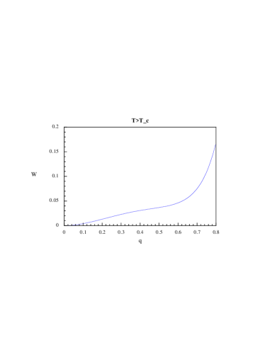
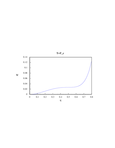
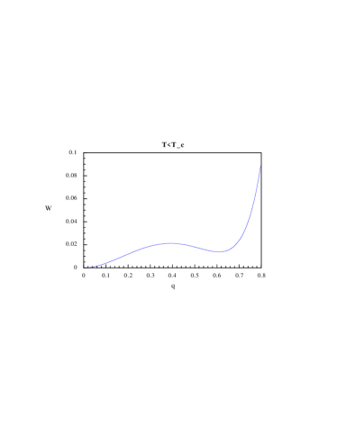
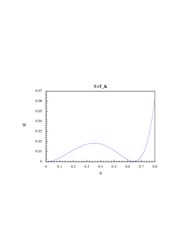
Figure 3: Qualitative behaviour of the potential $W(q)$, in the four regions $T>T_{c}$, $T=T_{c}$, $T_{K}<T<T_{c}$ and $T=T_{K}$. In these graphs the metastable part can be easily identified by remembering that $W(q)$ must be a convex function of $q$.

Fig. 4 shows the expectation value of $q$ as function of $\epsilon$ in the corresponding four temperature ranges. The results for the potential $W(q)$ in the unstable region where its second derivative is negative and $q$ is a decreasing function of $\epsilon$ are a clear artefact of the mean field approximation, while the results in the metastable region correspond to phenomena that can be observed on time scales shorter than the lifetime of the metastable state.

The thermodynamic configurational entropy is the value of the potential $W(q)$ at the secondary minimum with $q\neq 0$ [36], and it can be defined only if the minimum do exist (i.e. for $T<T_{c}$). It is evident that the secondary minimum for $T>T_{k}$ is always in the metastable region. However if one would start from a large value of $\epsilon$ and would decrease $\epsilon$ to zero not too slowly, the system would not escape from the metastable region and one obtains a proper definition of the thermodynamic configurational entropy in this region $T>T_{K}$. In a similar way one could compute $q(\epsilon)$ in the region ($\epsilon>\epsilon_{c}$) where the high $q$ phase is thermodynamically stable and extrapolate it to $\epsilon\to 0$. The ambiguity in the definition of the thermodynamic configurational entropy at temperatures above $T_{k}$ becomes larger and larger when the temperature increases. It cannot be defined for $T>T_{c}$.

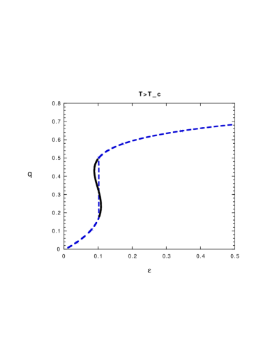
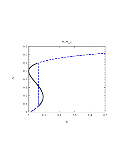
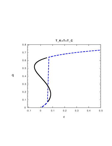
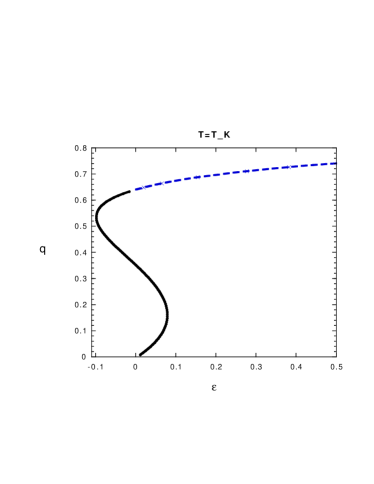
Figure 4: Qualitative behaviour of the order parameter $q$, measuring the typical distance to the reference configuration, versus the strength $\epsilon$ of the coupling to this reference configuration, in the four regions $T>T_{c}$, $T=T_{c}$, $T_{K}<T<T_{c}$ and $T=T_{K}$. The dashed line shows the true thermodynamically stable curve, where the full line is the metastable and the unstable part of the curve.

6.4 Numerical estimates of the configurational entropy

Most attempts at estimating numerically the thermodynamic configurational entropy start from the decomposition (28). The liquid entropy is estimated by a thermodynamic integration of the specific heat from the very dilute (ideal gas) limit. It turns out that in the deeply supercooled region the temperature dependence of the liquid entropy is well fitted by the law predicted in [32]: $S_{liq}(T)=aT^{-2/5}+b$, which presumably allows for a good extrapolation at temperatures $T$ which cannot be simulated. As for the ’valley’ entropy, it can be estimated as that of an harmonic solid. One needs however the vibration frequencies of the solid. These have been approximated by several methods, which are all based on some evaluation of the Instantaneous Normal Modes (INM) [38] in the liquid phase, and the assumption that the spectrum of frequencies does not depend much on temperature below $T_{K}$. Starting from a typical configuration of the liquid, one can look at the INM around it. In general there exist some negative eigenvalues (the liquid is not a local minimum of the energy) which one must take care of. Several methods have been tried: either keep only the positive eigenvalues, or one considers the absolute values of the eigenvalues [22, 23, 24]. Alternatively one can also consider the INM around the nearest inherent structure which has by definition a positive spectrum [22, 23, 24, 39]. The computation of the thermodynamic entropy, using its definition as a system coupled to a reference thermalized configuration, has also been studied in [22].

The results for the configurational entropy as a function of temperature are shown in fig. 5, for binary mixtures of soft spheres and of Lennard-Jones particles. The agreement with the analytical result obtained from the replicated fluid system is rather satisfactory, considering the various approximations involved both in the analytical estimate and in the numerical ones.

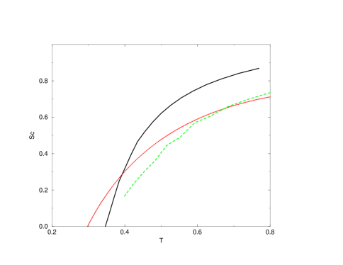
Figure 5: The configurational entropy versus temperature in binary mixtures of soft-spheres and of Lennard-Jones particles. The soft sphere result (left curve), from [22], compares the analytical prediction obtained within the harmonic resummation scheme (full line), to simulation estimates of $S_{liq}-S_{valley}$, where the valley entropy is that of a harmonic solid with INM eigenvalues projected onto positive eigenvalues (+), taken in absolute values ($\times$), or taken around the nearest inherent structure ($\ast$). The squares correspond to the numerical estimate of the thermodynamic configurational entropy obtained by studying the system coupled to a reference configuration (see text, and [22] for details). The Lennard-Jones result (right curve), shows as a full (black) curve the theoretical prediction obtained from the cloned molecular liquid approach[23, 24]. The dotted (green) curve is the result from the simulations of [23, 24] and the dashed (red) curve is the result from the simulations of [39]. Both simulations use the $S_{liq}-S_{valley}$ estimate where the harmonic solid vibration modes are approximated by the ones of the nearest inherent structure.

In a recent work, Sciortino Kob and Tartaglia [39] have computed the configurational entropy of inherent structures, $\Sigma_{is}(T)$, defined in (23), in binary Lennard-Jones system. Assuming that the free energy $-T\log Z(a)$ of an inherent structure $a$ ($Z(a)$ is defined in (22)) can be approximated by $E_{a}+\delta F(T)$, with a correction $\delta F$ which is nearly independent of $E_{a}$, then the logarithm of the probability of finding an inherent structure with a given energy $E_{IS}$ is given by $-\beta E_{IS}+\Sigma_{is}(E_{IS})+c^{t}$. One can thus deduce the $E_{IS}$ dependence of $\Sigma_{IS}$. Shifting the curves vertically in order to try to superimpose them with the thermodynamic configurational entropy, they have checked that all these curves coincide in the region of small enough energy, confirming thus that these two definitions of the configurational entropy agree at low enough energy or temperature. In fig. 6 we compare their result for the configurational entropy of inherent structures to the one obtained analytically, using the description of the molecular fluid of binary Lennard-Jones particles of [23, 24]. Apart from a small shift in the ground state energy which may have several origins (finite size effects, small uncertainties in the description of the correlation in the molecular fluid), the figures are in rather good agreement.

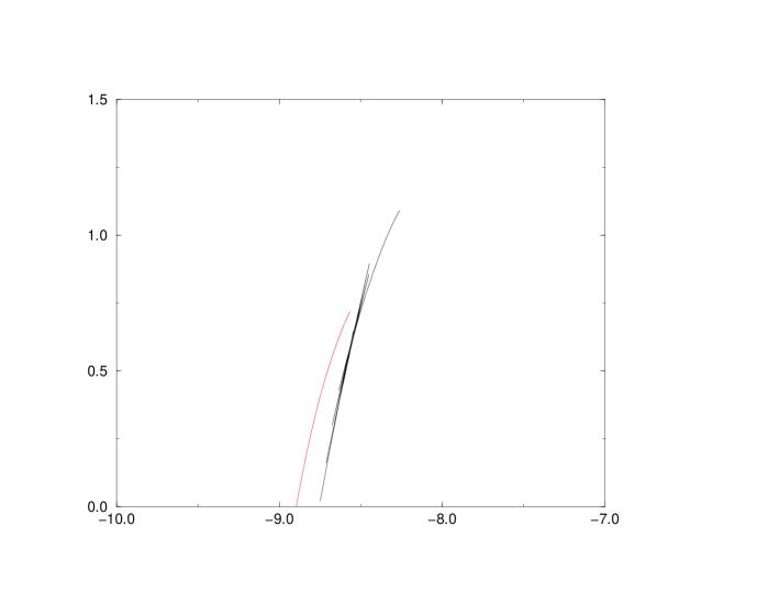
Figure 6: The left (red) curve is the configurational entropy of inherent structures versus energy for a binary Lennard-Jones fluid, computed numerically in [39] (with respect to the curve plotted in [39], the energies have been shifted in order to take into account the truncation of the Lennard-Jones potential used in the simulations of [39]). The right curve is the analytic prediction, using the description of the molecular fluid of binary Lennard-Jones particles of [23, 24]. There is a small shift in energy between the two curves, but the overall agreement is satisfactory.

7 Remarks

We believe that we have now a consistent scheme for computing the thermodynamic properties of glasses at equilibrium. What is needed is on the one hand some better approximations of the molecular liquid state, on the other hand some precise numerical results in the glass phase at equilibrium, as well as measurements of the fluctuation dissipation ratio in the out of equilibrium dynamics (which should give the value of $m$ [15]). Another obvious direction is to study, with the present methods, various types of interaction potentials, including some which are characteristic of strong glasses. Eventually, one would like to proceed to a first principle study of the out of equilibrium dynamics.

8 Acknowledgments

We wish to thank W. Kob for providing the data discussed in the last section, and for giving us the energy shift of the truncated Lennard-Jones problem, used in the comparison of fig. 6. We wish to thank P. Verrocchio for providing the analytic prediction shown in fig. 6.

9 References

References

- [1]
- [2] Recent reviews can be found in: C.A. Angell, Science, 267, 1924 (1995) and P.De Benedetti, ‘Metastable liquids’, Princeton University Press (1997). An introduction to the theory is: J.Jäckle, Rep.Prog. Phys. 49 (1986) 171.
- [3] A.W. Kauzman, Chem.Rev. 43 (1948) 219. A nice recent discussion can be found in R. Richert and C.A. Angell, J.Chem.Phys. 108 (1999) 9016.
- [4] G. Adams and J.H. Gibbs J.Chem.Phys 43 (1965) 139; J.H. Gibbs and E.A. Di Marzio, J.Chem.Phys. 28 (1958) 373.
- [5] In this sense, the rubber is a structural glass which is much closer to spin glasses, because of the quenched random links between the macromolecules. Theoretical studies of rubber are reviewed in P.M. Goldbart, H.E. Castillo and A. Zippelius Adv. Phys. 45 (1996) 393.
- [6] For a review, see M. Mézard, G. Parisi and M.A. Virasoro, Spin glass theory and beyond, World Scientific (Singapore 1987)
- [7] B. Derrida, Phys. Rev. B24, 2613 (1981)
- [8] D.J. Gross and M. Mézard, Nucl. Phys. B240 (1984) 431.
- [9] T.R. Kirkpatrick and P.G. Wolynes, Phys. Rev. A34, 1045 (1986); T.R. Kirkpatrick and D. Thirumalai, Phys. Rev. Lett. 58, 2091 (1987); T.R. Kirkpatrick and D. Thirumalai, Phys. Rev. B36, 5388 (1987); T.R. Kirkpatrick, D. Thirumalai and P.G. Wolynes, Phys. Rev. A40, 1045 (1989).
- [10] A. Crisanti, H. Horner and H.J. Sommers, Z. Physik B 92, 257 (1993).
- [11] J.-P. Bouchaud and M. Mézard; J. Physique I (France) 4 (1994) 1109. E. Marinari, G. Parisi and F. Ritort; J. Phys. A27 (1994) 7615; J. Phys. A27 (1994) 7647.
- [12] P.Chandra, L.B.Ioffe and D.Sherrington, Phys. Rev. lett. 75 (1995) 713, and cond-mat/9809417. P.Chandra, M.V. Feigelman and L.B.Ioffe, Phys. Rev. lett. 76 (1996) 4805.
- [13] E. Marinari, G. Parisi and F. Ritort, cond-mat/9410089. S. Franz and J. Hertz, Phys. Rev. Lett. 74, 2114 (1995).
- [14] L. F. Cugliandolo and J.Kurchan, Phys. Rev. Lett. 71, 1 (1993).
- [15] S. Franz, M. Mézard, G. Parisi and L. Peliti, Phys. Rev. Lett. 81 1758 (1998); The response of glassy systems to random perturbations: A bridge between equilibrium and off-equilibrium, cond-mat/9903370, to appear in J.Stat.Phys.
- [16] G. Parisi Phys.Rev.Lett. 78(1997)4581.
- [17] W. Kob and J.-L. Barrat, Phys.Rev.Lett. 79 (1997) 3660.
- [18] J.-L. Barrat and W. Kob, cond-mat/9806027.
- [19] M. Mézard and G. Parisi, Phys. Rev. Lett. 82, 747 (1998).
- [20] M. Mézard, Physica A 265, 352 (1999).
- [21] M. Mézard and G. Parisi J. Chem. Phys. 111, 1076 (1999).
- [22] B. Coluzzi, M. Mézard, G. Parisi and P. Verrocchio, Thermodynamics of binary mixture glasses, cond-mat/9903129.
- [23] B. Coluzzi, G. Parisi and P. Verrocchio, Lennard-Jones binary mixture: a thermodynamical approach to glass transition, cond-mat/9904124.
- [24] B. Coluzzi, G. Parisi and P. Verrocchio, The thermodynamical liquid-glass transition in a Lennard-Jones binary mixture, cond-mat/9906124.
- [25] An introduction to recent work on Kepler’s conjecture can be found in: www.math.lsa.umich.edu/ hales/countdown/.
- [26] L. Angelani, G. Parisi, G. Ruocco and G. Viliani, cond-mat/9904125.
- [27] T.M. Nieuwenhuizen, Phys.Rev.Lett. 79 (1997) 1317.
- [28] M. Goldstein, J. Chem. Phys. 51, 3728 (1969); F.H. Stillinger, Science 267 (1995) 1935, and references therein. Recent includes: S. Sastry, P.G. Debenedetti and F.H. Stillinger, Nature 393, 554 (1998), W. Kob, F. Sciortino and P. Tartaglia, cond-mat/9905090; F. Sciortino, W. Kob and P. Tartaglia, cond-mat/9906278; S. Büchner and A. Heuer, cond-mat/9906280.
- [29] R. Monasson, Phys. Rev. Lett. 75, 2847 (1995).
- [30] M. Mézard, G. Parisi and A. Zee Spectra of Euclidean Random Matrices, cond-mat/9906135.
- [31] A. Cavagna, I. Giardina and G. Parisi, Analytic computation of the Instantaneous Normal Modes spectrum in low density liquids (cond-mat/9903155), Phys.Rev.Lett. to be published.
- [32] Y.Rosenfeld and P. Tarazona, Mol.Phys. 95, 141 (1998).
- [33] G.Parisi, cond-mat/9905318.
- [34] B. Bernu, J.-P. Hansen, Y. Hitawari and G. Pastore, Phys. Rev. A 36, 4891 (1987). J.-L. Barrat, J.-N. Roux and J.-P. Hansen, Chem. Phys. 149, 197 (1990). J.-P. Hansen and S. Yip, Trans. Theory and Stat. Phys. 24, 1149 (1995).
- [35] See the talk of Speedy at this conference and references therein.
- [36] S. Franz ang G. Parisi, J. Physique I 5 (1995) 1401; Phys.Rev.Lett. 79 (1997) 2486.
- [37] M.Cardenas, S. Franz and G. Parisi, cond-mat/9712099.
- [38] T. Keyes, J. Chem. Phys. A101 (1997) 2921.
- [39] F. Sciortino, W. Kob and P. Tartaglia, Inherent structure entropy of supercooled liquids, cond-mat/9906081. See also Sciortino’s contribution to this volume.