Theory of Four Wave Mixing of Matter Waves from a Bose-Einstein Condensate

Abstract

A recent experiment [Deng et al., Nature 398, 218(1999)] demonstrated four-wave mixing of matter wavepackets created from a Bose-Einstein condensate. The experiment utilized light pulses to create two high-momentum wavepackets via Bragg diffraction from a stationary Bose-Einstein condensate. The high-momentum components and the initial low momentum condensate interact to form a new momentum component due to the nonlinear self-interaction of the bosonic atoms. We develop a three-dimensional quantum mechanical description, based on the slowly-varying-envelope approximation, for four-wave mixing in Bose-Einstein condensates using the time-dependent Gross-Pitaevskii equation. We apply this description to describe the experimental observations and to make predictions. We examine the role of phase-modulation, momentum and energy conservation (i.e., phase-matching), and particle number conservation in four-wave mixing of matter waves, and develop simple models for understanding our numerical results.

I Introduction

Nonlinear optics has been made possible by the nonlinear nature of the interaction between light and matter and by the development of intense light sources that can probe the nonlinear regime of this interaction. Nonlinear optical processes include three- and four-wave mixing (4WM) processes (e.g., second harmonic generation and third harmonic generation). In 4WM three waves (or light pulses) mix to produce a fourth. In this paper we detail our studies of 4WM of coherent matter waves. Trippenbach et al. [1] proposed a 4WM experiment using three colliding Bose-Einstein condensate (BEC) wavepackets with different momenta. Deng et al. [2] successfully demonstrated 4WM in an experiment with three BEC wavepackets, which interact in a nonlinear manner to make a fourth BEC wavepacket. Here we greatly elaborate on and further develop the theory and describe numerical simulations of the 4WM output that agree well with the experimental measurements of  [2].

The experimental study of nonlinear atom optics is made possible by the advent of Bose-Einstein condensation of dilute atomic gases [3, 4] and the atom “laser” [5], a source of coherent matter-waves analogous to the output of optical lasers. A set of optical light pulses incident on a parent condensate with momentum ${\bf P}_{1}={\bf 0}$ can, by Bragg scattering [6], create two new daughter BEC wavepackets with momenta ${\bf P}_{2}$ and ${\bf P}_{3}$. Four-wave mixing in a single spin-component condensate occurs as a result of the nonlinear self-interaction term in the Hamiltonian for a BEC when three such BEC wavepackets with momenta ${\bf P}_{1}$, ${\bf P}_{2}$, and ${\bf P}_{3}$ collide and interact. The nonlinear self-interaction can generate a new BEC wavepacket with a new momentum ${\bf P}_{4}={\bf P}_{1}-{\bf P}_{2}+{\bf P}_{3}$.

The possibility of nonlinear effects in atom optics has been long recognized [7]. Goldstein et al. [8] proposed that phase conjugation of matter waves should be possible in analogy to this phenomenon in nonlinear optics, including the case of multiple spin-component condensates [9]. They considered the case where a “probe” BEC wavepacket interacts with two counter-propagating “pump” wavepackets to generate a fourth that is phase conjugate to the probe, where the probe is weak and causes negligible depletion of the pump. Law et al. [10] also suggested analogies between interactions in multiple spin-component condensates and four-wave mixing. Goldstein and Meystre [11] develop a theory of 4WM in multicomponent BECs based on an algebraic angular momentum approach to obtain the modes of the coupled operator equations. Our treatment for a single spin-component condensate is based on the time-dependent Gross-Pitaevskii equation (GPE), which has proved to be highly successful in describing the properties of a variety of actual BEC experiments [4]. Thus, our treatment is for a zero temperature condensate. It also can describe 4WM with or without the presence of a trapping potential.

The nature of 4WM in BEC collisions of matter waves is unlike 4WM for optical wavepacket collisions in dispersive media  [12, 13, 14]. The nonlinearity in the case of BEC is introduced by collisions rather than by interaction with an external medium, and the momentum and energy constraints imposed are different in the two cases. The kinetic energy of massive particle waves is quadratic in the wavevector of the particles and given by $(\hbar{\bf k})^{2}/2m$, whereas the energy of a photon is linear in the vacuum wavevector of the photon, ${\bf k}$, and is given by $\hbar c|{\bf k}|$. Moreover, the momentum of massive particle waves is linear in the wavevector of the particles and given by $\hbar{\bf k}$, whereas for light in a dispersive medium, it is proportional to the product of the frequency of the light, $\omega=c|{\bf k}|$ and the refractive index, $n(\omega)$, where the refractive index depends upon frequency (and the propagation direction in non-isotropic media). Hence, conservation of energy does not in general guarantee conservation of momentum in optical 4WM. Clearly, complications involving the properties of an additional medium does not arise in the BEC case. In any case, the creation of new BEC wavepackets in 4WM is limited to cases when momentum, energy and particle number conservation are simultaneously satisfied.

In this paper we develop a general three-dimensional (3D) description of four-wave mixing in single-spin-component Bose-Einstein condensates using a mean-field approach similar to the time-dependent GPE, also known as the nonlinear Schrödinger equation [4]. We introduce the slowly-varying-envelope approximation (SVEA), a very powerful tool that not only gives insight into the nature of 4WM but also gives a set of four coupled equations for the four interacting BEC waves that are more computationally tractable for numerical simulations of the time-dependent dynamics. Section II explains the experimental situation we have in mind and develops the basic theoretical methods. Section III describes the results of our numerical calculations and compares these to the NIST experiment [2]. Finally, in Sec. IV we present a summary and conclusion.

II Theory of Matter-Wave Four-Wave Mixing

In this section we describe the theoretical tools used in our study of 4WM of matter waves. Section II A reviews how high momentum components of a BEC can be formed using optical Bragg pulses to prepare the initial configuration for the “half collision” event. Section II B specifies the parameters that describe the strength of the various physical effects that play a role in 4WM: diffraction, potential energy, nonlinear self-energy, and collisions between the different momentum wavepackets. This Section also describes how to transform between 1D, 2D and 3D calculations involving the GPE. This is important because, without the slowly-varying-envelope approximation (SVEA) that we introduce below, full 3D calculations are too computationally expensive to carry out for the actual experimental conditions. Hence, the SVEA must be explicitly checked in 2D against the full GP solution. Section II C describes the details of the SVEA approximation for 4WM. Then Section II D introduces a simple estimate for the 4WM output. Finally, Section II E shows how the effect of elastic scattering between atoms in different momentum wavepackets can be accounted for. This process causes loss of atoms from the wavepackets and lowers the 4WM output.

Let us consider three BEC wavepackets moving with central momenta ${\bf P}_{1}$, ${\bf P}_{2}$, and ${\bf P}_{3}$. Such moving wavepackets can be created, for example, by optically-induced Bragg diffraction of a condensate [6]. If these three wavepackets overlap spatially, the self-energy of the atoms can produce matter-wave 4WM, just as the third-order Kerr type nonlinearity can produce optical 4WM in nonlinear media. One can imagine a number of scenarios in which 4WM can occur in matter-wave interactions. One can consider a “whole collision” in which three initially separated BEC wavepackets collide together at the same time, or a “half collision” in which the wavepackets are initially formed in the same condensate at (nearly) the same time. Although we considered the “whole collision” case in Ref. [1], the “half collision” case is easier to realize experimentally [2] using the above-mentioned Bragg diffraction technique [6]. In what follows, we consider only this configuration, in which the three wavepackets initially overlap because they have been created as copies of the initial condensate. These wavepackets have different non-vanishing central momenta and therefore they fly apart from one another after they have been created.

Fig. 1a shows the basic configuration in momentum space of the wavepackets which we consider here. Two daughter condensate wavepackets with momenta ${\bf P}_{2}$ and ${\bf P}_{3}$ are created from a parent condensate with mean momentum ${\bf P}_{1}=0$. Fig. 2a shows these three momenta in the lab frame in which the experiment is carried out at two different times: during the early stage of the “half collision” when they still overlap spatially, and at a later time when they have spatially separated into four distinct wavepackets. We let ${\bf P}_{3}$ lie along the $x$-axis of the coordinate system, and ${\bf P}_{2}$ make some angle $\theta$ with respect to the $x$-axis. Nonlinear 4WM creates a fourth wavepacket with momentum ${\bf P}_{4}={\bf P}_{1}-{\bf P}_{2}+{\bf P}_{3}$. We demonstrate below in Sec. II C that four-wave mixing of matter waves is only possible if there exists a coordinate frame in which the mixing is degenerate, that is, all four ${\bf P}^{\prime}_{i}$ values in this frame have the same magnitude. Fig. 2b shows the degenerate frame corresponding to a moving frame with velocity ${\bf V}_{deg}=({\bf P}_{1}+{\bf P}_{3})/(2m)$, where $m$ is the atomic mass. The total momentum is zero in the degenerate frame, and the wavepackets move in oppositely moving pairs. The angle $\theta^{\prime}$ between the vectors ${\bf P}_{2}^{\prime}$ and ${\bf P}_{3}^{\prime}$ is arbitrary. In the laboratory frame, the angle $\theta$ is given by $\theta=\theta^{\prime}/2$, and the length of the vector ${\bf P}_{2}$ is given by $|{\bf P}_{2}|=|{\bf P}_{3}|\cos(\theta)$. Fig. 1b shows a set of different possible values of ${\bf P}_{2}$.

A Bragg Pulse Creation of High Momentum Components

We assume that the condensate has only a single spin-component, and that its dynamics can be described by the GPE, which is known to provide an excellent account of condensate properties [4]:

$$i\hbar\frac{\partial\Psi({\bf r},t)}{\partial t}=(T_{{\bf r}}+V({\bf r},t)+NU_{0}|\Psi|^{2})\Psi({\bf r},t),$$ (1)

where $T_{{\bf r}}=\frac{-\hbar^{2}}{2m}\nabla_{\bf r}^{2}$ is the kinetic energy operator, $V({\bf r},t)$ is the external potential imposed on the atoms, $NU_{0}=N\frac{4\pi a_{0}\hbar^{2}}{m}$ is the atom-atom interaction strength that is proportional to the $s$-wave scattering length $a_{0}$ (assumed to be positive), $m$ is the atomic mass, and $N$ is the total number of atoms. The numerical methods for solving the GPE are described below in Sec. III.

First, we use the GPE to obtain the ground state condensate in the trapping potential at time $t=0$, $\Psi({\bf r},t=0)$. This condensate wavefunction is centered around ${\bf r}={\bf 0}$, and normalized to unity. We assume, as is the case in the NIST experiments [2], that the trapping potential $V({\bf r},t)$ is turned off at $t=0$ and that the condensate is allowed to evolve under the influence of only the mean-field interaction until time $t_{1}$. This includes the special case $t_{1}=0$. We could equally well treat the case of leaving the trap on, and we would obtain similar results. Eq. (1) determines the evolved condensate wavefunction, $\Psi({\bf r},t_{1})$. After this period of free evolution, the Bragg pulses are applied to create the wavepackets with momenta ${\bf P}_{1}$, ${\bf P}_{2}$ and ${\bf P}_{3}$. The momentum differences $|{\bf P}_{i}-{\bf P}_{j}|$ are much larger than the momentum spread of the initial parent BEC wavepacket. The experimental time scale $\delta t$ for creating these wavepackets is short ($\approx$ 70 $\mu$s) compared to the time scale on which the wavepackets evolve. The state at $t_{2}=t_{1}+\delta t$ provides the initial condition for subsequent evolution of these three wavepackets as they undergo nonlinear evolution.

The initial state at $t_{2}$ immediately after the Bragg pulse sequences can be approximated in a number of ways. In principle one could set up a set of coupled GPEs for the ground and excited atomic state components and explicitly include the effect of coupling the light field to the excited electronic state. A simpler approach would be to carry out an adiabatic elimination of the excited state and develop an effective light-shift potential in which the ground state atoms move. If such approaches are carried out in this case, they show that the light acts as a “sudden” perturbation such that each of the wavepackets with central momenta ${\bf P}_{1}$, ${\bf P}_{2}$ and ${\bf P}_{3}$ is to a very good approximation simply a “copy” of the parent condensate at $t=t_{1}$ [15]. Thus, the initial condition immediately after the application of the Bragg pulses can be approximated as being comprised of three BEC wavepackets,

$$\Psi({\bf r},t_{2})=\Psi({\bf r},t_{1})\sum_{i=1}^{3}f_{i}^{1/2}\exp(i{\bf P}_{i}\cdot{\bf r}/\hbar),$$ (2)

where $f_{i}=N_{i}/N$ is the fraction of atoms in wavepacket $i$, and $\sum_{i=1}^{3}f_{i}=1$ so the norm of $\Psi$ remains unity.

After the formation of the wavepackets with momenta ${\bf P}_{1}$, ${\bf P}_{2}$ and ${\bf P}_{3}$, the initial wavefunction in Eq. (2) evolves, and the wavepackets with the different momenta separate. During this separation,the nonlinear term in the GPE generates a wavepacket with central momentum ${\bf P}_{4}={\bf P}_{1}-{\bf P}_{2}+{\bf P}_{3}$, as long as the constraints discussed in relation to Figs. 1 and 2 are satisfied. Energy and momentum are conserved during the wavepacket evolution. This can be readily checked by verifying that $dE(t)/dt=0$ and $d{\bf P}(t)/dt=0$, where

$$E(t)=\langle\Psi(t)|(T_{{\bf r}}+\frac{1}{2}U_{0}|\Psi|^{2})|\Psi(t)\rangle,$$ (3)

is the energy per particle and

$${\bf P}(t)=-i\hbar\langle\Psi(t)|\mbox{\boldmath$\nabla$}|\Psi(t)\rangle\ ,$$ (4)

is the momentum per particle. We have verified numerically that energy and momentum are indeed conserved in our calculations described in Section III.

B Characteristic Time Scales, and Dimensionless Parameters

In this subsection we discuss characteristic time scales that can be used to estimate the importance of the various effects occurring during the dynamics for a particular set of experimental parameters. It is convenient to use the Thomas–Fermi (TF) approximation [4] to give quantitative estimates of the size of the condensate and the time scales characterizing the dynamics. In the TF approximation, one neglects the kinetic energy operator in the time-independent nonlinear Schrödinger equation,

$$\mu\Psi=(T_{{\bf r}}+V({\bf r},t)+NU_{0}|\Psi|^{2})\Psi,$$ (5)

where $\mu$ is the chemical potential, to obtain the following analytical expression for the wavefunction: $|\Psi({\bf r})|^{2}=\frac{\mu-V({\bf r})}{NU_{0}}$ for ${\bf r}$ such that $V({\bf r})\leq\mu$ and $\Psi({\bf r})=0$ otherwise. The TF approximation is valid for sufficiently large numbers of atoms $N$. It is convenient to define the geometric average of the oscillator frequencies for an asymmetric harmonic potential as $\bar{\omega}=(\omega_{x}\omega_{y}\omega_{z})^{1/3}$. The size of the condensate is then given by the TF radius $r_{TF}=\sqrt{2\mu/(m\bar{\omega})}$, where the TF approximation to the chemical potential $\mu$ is determined by the normalization of the wavefunction to unity and is given by $\mu=\frac{1}{2}\left(\frac{15U_{0}N}{4\pi}\right)^{2/5}(m\bar{\omega}^{2})^{3/5}$. Hence, the TF radius $r_{TF}$ scales with $N$ as $N^{1/5}$. The size of the TF wavepacket in the $i=$ $x$, $y$, and $z$ directions is $r_{TF}(i)=(\bar{\omega}/\omega_{i})r_{TF}$.

In order to estimate the importance of the various terms in the GPE, we set $V=0$ for free wavepacket evolution and rewrite Eq. (1) in terms of characteristic time scales $t_{DF}$ for diffraction, and $t_{NL}$ for the nonlinear interaction, in the following manner [1, 18, 19]:

$$\frac{\partial\Psi}{\partial t}=i\left[\frac{r_{TF}^{2}}{t_{DF}}\,(\frac{\partial^{2}}{\partial x^{2}}+\frac{\partial^{2}}{\partial y^{2}}+\frac{\partial^{2}}{\partial z^{2}})-\frac{1}{t_{NL}}\,\frac{|\Psi|^{2}}{|\Psi_{m}|^{2}}\right]\Psi.$$ (6)

The diffraction time and the nonlinear interaction time are given by $t_{DF}=2mr_{TF}^{2}/\hbar$, $t_{NL}=(NU_{0}|\Psi_{m}|^{2}/\hbar)^{-1}$, respectively. Here $|\Psi_{m}|^{2}$ is the maximum value of $|\Psi({\bf r})|^{2}$, i.e., $|\Psi_{m}|^{2}=|\Psi({\bf 0})|^{2}$; hence in the TF approximation, $t_{NL}^{-1}=\mu/\hbar$. The smaller the characteristic time, the larger is the corresponding term in the GPE. We also define the collision duration time $t_{col}=(2r_{TF})/v$, where ${\bf v}=({\bf P}_{3}-{\bf P}_{1})/m$ is the initial relative velocity of wavepackets 1 and 3. Thus, $t_{col}$ is the time it takes the wavepackets 1 and 3 to move so that they just touch at their TF radii, and therefore no longer overlap. The ratio $t_{col}/t_{NL}$ gives an indication of the strength of the nonlinearity during the collision. The larger the ratio of $t_{col}/t_{NL}$, the stronger the effects of the nonlinearity during the overlap of the wavepackets. These characteristic times stand in the ratios $t_{DF}:t_{col}:t_{NL}=1:\frac{\lambda}{2\pi r_{TF}}:\frac{r_{TF}}{6a_{0}N}$, where $\lambda$ is the De Broglie wavelength associated with the wavepacket velocity $v$. Experimental condensates with $t_{col}/t_{NL}\gg 1$ can be readily achieved. Thus, the nonlinear term will have time to act while the BEC wavepackets remain physically overlapped during a collision. Another relevant time scale in the dynamics is the characteristic condensate expansion time, $t_{exp}=\bar{\omega}^{-1}$. In the typical experiments modeled below, $t_{DF}\gg t_{exp}>t_{col}>t_{NL}$.

In addition to time scales, there are several natural length scales that are important: the size $r_{TF}$ of the condensate, the scale $(\Delta k)^{-1}$ of phase variation across the parent condensate as it expands and develops a momentum spread $\hbar\Delta k$ due to the mean field potential, and the scale $(k^{\prime})^{-1}$ of phase variation due to the fast imparted momentum $P^{\prime}=\hbar k^{\prime}$, where $P^{\prime}$ is the common magnitude of the momentum for the packets in the degenerate frame (Fig. 1). These stand in the relation $(k^{\prime})^{-1}\ll(\Delta k)^{-1}\ll r_{TF}$. The grid spacings in numerical calculations are determined by the necessity to resolve the wavefunction on its fastest scale of variation. Thus, using the form of Eq. (2) for $\Psi$ requires a grid smaller than $(k^{\prime})^{-1}$. This requirement limits practical calculations to 2 dimensions (2D). We will introduce an approximation in the next section that allows three dimensional (3D) calculations by eliminating the rapidly varying phase factors from the equations to be solved.

We find it convenient to use reduced dimensionless variables to calculate the dynamics. The most commonly used set of reduced dimensionless variables in BEC problems involves using “trap units” [4]. Here however, except for determining the initial conditions at $t=0$, the trap potential is turned off, and trap units are not particularly relevant. Since we do both 2D and 3D calculations, some care is needed in developing a set of units. The primary requirement to simulate 3D experiments with a 2D model is that the relations between the characteristic timescales, $t_{DF}$, $t_{col}$ and $t_{NL}$, are as determined by experiment. We have done this by scaling the solution of the $d$–dimensional time-dependent GPE by a $d$–dimensional volume so that the coefficient of the nonlinear term depends only on the dimension and the chemical potential $\mu$. By scaling the condensate wavefunction as $\Psi=\bar{\Psi}/\sqrt{r_{TF}^{d}}$, the $d$–dimensional time-dependent GPE for a harmonic potential with frequencies $\omega_{j}$, $j=1\dots d$ can be written as

$$i\hbar\frac{\partial\bar{\Psi}\left({\bf r}\right)}{\partial t}=-\frac{\hbar^{2}}{2m}\sum_{j=1}^{d}\frac{\partial^{2}\bar{\Psi}}{\partial x_{j}^{2}}+\left(\sum_{j=1}^{d}\frac{1}{2}m\omega_{j}^{2}x_{j}^{2}\right)\bar{\Psi}\left({\bf r}\right)+\left(\frac{\pi^{d/2}}{\Gamma(2+\frac{d}{2})}\right)\mu_{{\rm TF}}\left|\bar{\Psi}\left({\bf r}\right)\right|^{2}\bar{\Psi}\left({\bf r}\right)\ .$$ (7)

Here $\bar{\Psi}$ is dimensionless for any $d$, and the known $\mu_{TF}$ for the 3D problem can be transferred to an equivalent time-dependent GPE for a 2D calculation. Furthermore, if we define the reduced unit of length, $x_{R}$, to be $x_{R}=r_{TF}$, define the unit of time, $t_{R}$, such that $t_{R}=mx_{R}^{2}/(2\hbar)$, and use the normalization condition: $\int|\bar{\Psi}|^{2}\,d^{d}{\bf r}/x_{R}^{d}=1$, we preserve the ratios between the most important time scales of the problem. The nonlinear time scale, $t_{NL}$ depends only on $\mu_{TF}$ and is independent of dimension. The specific relations between the 3D nonlinear coupling parameter $U_{0}^{3D}$ multiplying $\left|\bar{\Psi}\left({\bf r}\right)\right|^{2}\bar{\Psi}\left({\bf r}\right)$ in Eq. (7) and $U_{0}^{1D}$ and $U_{0}^{2D}$, the respective self-energy parameters in 1D and 2D are: $U_{0}^{1D}=\frac{5}{2\pi}U_{0}^{3D}$, and $U_{0}^{2D}=\frac{15}{16}U_{0}^{3D}$. These values for $U_{0}^{d}$ insure that the chemical potential $\mu_{TF}$ (and all the time scales) are the same as in 3D.

C Slowly Varying Envelope Approximation

Let us consider the case when the total wavefunction consists of four wavepackets moving with different central momenta ${\bf P}_{i}=\hbar{\bf k}_{i},i=1,\ldots,4$. We write the wavefunction as

$$\Psi({\bf r},t)=\sum_{i=1}^{4}\Phi_{i}({\bf r},t)\,\exp{[i({\bf k}_{i}{\bf r}-\omega_{i}t)]}\,,$$ (8)

in order to separate out explicitly the fast oscillating phase factors representing central momentum $\hbar{\bf k}_{i}$ and kinetic energy $E_{i}=\hbar\omega_{i}=\hbar^{2}k_{i}^{2}/2m$. The slowly varying envelopes $\Phi_{i}({\bf r},t)$ vary in time and space on much longer scales than the phases. The number of atoms in each wavepacket is $N_{i}=N\int_{V}|\Phi_{i}({\bf r},t)|^{2}d^{3}{\bf r}$, and $\sum_{i=1}^{4}N_{i}=N$ is a constant. Although the slowly varying envelope $\Phi_{4}({\bf r},t=0)$ is unpopulated initially, it evolves and becomes populated as a result of the 4WM process. If we substitute the expanded form of the wavefunction in Eq. (8) into the GPE, collect terms multiplying the same phase factors, multiply by the complex conjugate of the appropriate phase factors, and neglect all terms that are not phase matched (phase matched terms have stationary phases, do not oscillate, and satisfy Eqs. (12-13) below), we obtain a set of coupled equations for the slowly varying envelopes $\Phi_{i}({\bf r},t)$:

$$\left(\frac{\partial}{\partial t}+(\hbar{\bf k}_{i}/m)\cdot\mbox{\boldmath$\nabla$}+\frac{i}{\hbar}(-\frac{\hbar^{2}}{2m}\nabla^{2}+V({\bf r},t))\right)\Phi_{i}({\bf r},t) = -\frac{i}{\hbar}NU_{0}\sum_{i^{*}jj^{*}}\delta({\bf k}_{i}+{\bf k}_{i^{*}}-{\bf k}_{j}-{\bf k}_{j^{*}})\times$$ (11)

$$\delta(\omega_{i}+\omega_{i^{*}}-\omega_{j}-\omega_{j^{*}})\times$$

$$\Phi_{j^{*}}({\bf r},t)\Phi_{i^{*}}^{*}({\bf r},t)\Phi_{j}({\bf r},t)\ ,$$

where the delta-functions represent Kronecker delta-functions that are unity when the argument vanishes. Mixing between different momentum components can result from the nonvanishing nonlinear terms in Eq. (11), which satisfy the phase matching constraints required by momentum and energy conservation:

$${\bf k}_{i}+{\bf k}_{i^{*}}-{\bf k}_{j}-{\bf k}_{j^{*}} = 0,\,\,\,\,\,\,\,\,\,\,$$ (12)

$$k^{2}_{i}+k^{2}_{i^{*}}-k^{2}_{j}-k^{2}_{j^{*}} = 0\ .$$ (13)

Each of the indices $i,i^{*},j,j^{*}$ may take any value between 1 and 4. Eqs. (12) and (13) are automatically satisfied in two cases: (a) $i=i^{*}=j=j^{*}$ (all indices are equal), or (b) $j=i\neq j^{*}=i^{*}$ (two pairs of equal indices). The corresponding terms describe what is called in nonlinear optics cross and self modulation terms respectively. The cross and self phase modulation terms do not involve particle exchange between different momentum components. In the absence of the trapping potential they modify both amplitude and phase of the wavepacket through the mean field interaction. Particle exchange between different momentum wavepackets occurs only when all four indices in Eq. (11) are different, and conservation of momentum and energy of the atoms participating in the exchange process occurs. A set of coupled equations involving wave mixing between the various momentum components is therefore obtained.

The momentum conservation of Eq. (12) implies ${\bf k}_{i}+{\bf k}_{i^{*}}={\bf k}_{j}+{\bf k}_{j^{*}}=$ $\kappa$. It is always possible to construct a special reference frame, which we call the degenerate frame, where $\kappa$$=0$. Consequently, in this frame ${\bf k}_{i}=-{\bf k}_{i^{*}}$ and ${\bf k}_{j}=-{\bf k}_{j^{*}}$. In addition energy conservation in Eq. (13) imposes the condition $|{\bf k}_{j}|=|{\bf k}_{i}|$ in the degenerate frame. In this frame all four momenta are equal in magnitude and can be divided into two pairs of opposite vectors. This explains the use of the conjugated pairs of symbols $(i,i^{*})$ and $(j,j^{*})$ in our notation. The total number of particles, in all wavepackets, is a conserved quantity. The geometrical configuration of the wavepacket momenta in the degenerate frame are illustrated in Fig. 2b. In the figure we see two pairs of conjugate wavepackets (1,3) and (2,4). All four momenta are equal in magnitude and momenta ${\bf P}_{1}^{\prime}$ and ${\bf P}_{3}^{\prime}$ are opposite as are the momenta ${\bf P}_{2}^{\prime}$ and ${\bf P}_{4}^{\prime}$. The angle $\theta$ depicted in the figure is completely arbitrary. However, $\theta\approx 0$ is not allowed, since the wavepackets would no longer be distinguishable. Fig. 1b shows a range of possible ${\bf P}_{2}$ values for wavepackets in the lab frame that satisfy the phase-matching conditions in Eqs. (12) and (13). These conditions only allow $|{\bf P}_{2}|=|{\bf P}_{3}|\cos{(\theta)}$.

4WM can be viewed as a process in which one particle is annihilated in each wavepacket belonging to an initially populated pair of wavepackets and simultaneously one particle is created in each of two wavepackets of another pair, one of which is initially populated and the other (wavepacket 4) is initially unpopulated. Hence, using Fig. 2b in the moving degenerate frame, 4WM removes one atom from each of the “pump” wavepackets 1 and 3, and places one atom in the “probe” wavepackets 2 and one atom in the 4WM output wavepacket 4. This picture is a consequence of the nature of the nonlinear terms in the four SVEA equations. It is this bosonic stimulation of scattering that mimics the stimulated emission of photons from an optical nonlinear medium.

The full SVEA equations for 4WM are explicitly given by:

$$\left(\frac{\partial}{\partial t}+(\hbar{\bf k_{1}}/m)\cdot\mbox{\boldmath$\nabla$}+\frac{i}{\hbar}(\frac{-\hbar^{2}}{2m}\nabla^{2}+V({\bf r},t))\right)\Phi_{1}({\bf r},t)=$$ (14)

$$-\frac{i}{\hbar}NU_{0}(|\Phi_{1}|^{2}+2|\Phi_{2}|^{2}+2|\Phi_{3}|^{2}+2|\Phi_{4}|^{2})\Phi_{1}-\frac{i}{\hbar}NU_{0}\Phi_{4}\Phi_{2}\Phi_{3}^{*}\ ,$$ (15)

$$\left(\frac{\partial}{\partial t}+(\hbar{\bf k_{2}}/m)\cdot\mbox{\boldmath$\nabla$}+\frac{i}{\hbar}(\frac{-\hbar^{2}}{2m}\nabla^{2}+V({\bf r},t))\right)\Phi_{2}({\bf r},t)=$$ (16)

$$-\frac{i}{\hbar}NU_{0}(|\Phi_{2}|^{2}+2|\Phi_{1}|^{2}+2|\Phi_{3}|^{2}+2|\Phi_{4}|^{2})\Phi_{2}-\frac{i}{\hbar}NU_{0}\Phi_{4}^{*}\Phi_{1}\Phi_{3}\ ,$$ (17)

$$\left(\frac{\partial}{\partial t}+(\hbar{\bf k_{3}}/m)\cdot\mbox{\boldmath$\nabla$}+\frac{i}{\hbar}(\frac{-\hbar^{2}}{2m}\nabla^{2}+V({\bf r},t))\right)\Phi_{3}({\bf r},t)=$$ (18)

$$-\frac{i}{\hbar}NU_{0}(|\Phi_{3}|^{2}+2|\Phi_{1}|^{2}+2|\Phi_{2}|^{2}+2|\Phi_{4}|^{2})\Phi_{3}-\frac{i}{\hbar}NU_{0}\Phi_{4}\Phi_{1}^{*}\Phi_{2}\ ,$$ (19)

$$\left(\frac{\partial}{\partial t}+(\hbar{\bf k_{4}}/m)\cdot\mbox{\boldmath$\nabla$}+\frac{i}{\hbar}(\frac{-\hbar^{2}}{2m}\nabla^{2}+V({\bf r},t))\right)\Phi_{4}({\bf r},t)=$$ (20)

$$-\frac{i}{\hbar}NU_{0}(|\Phi_{4}|^{2}+2|\Phi_{1}|^{2}+2|\Phi_{2}|^{2}+2|\Phi_{3}|^{2})\Phi_{4}-\frac{i}{\hbar}NU_{0}\Phi_{1}\Phi_{2}^{*}\Phi_{3}\ .$$ (21)

The left hand side of these equations describes the motion of the wavepackets due to their kinetic and potential energies. The right hand side describes the effect of the phase matched nonlinear interaction terms. The last term on the right hand side of each of the SVEA equations is a source term which either creates or destroys atoms in the wavepacket being propagated. The other terms on the right hand side of the equations account for the self- and cross-phase modulation. These phase modulation terms provide an effective potential for each wavepacket that accelerates the atoms in it and modifies its internal momentum distribution.

Before we propagate the SVEA equations, the initial wavefunction of the parent condensate is determined using the time-dependent GPE. First, the propagation is in imaginary time to obtain the initial eigenstate in the presence of the magnetic potential. Then, after turning off the magnetic potential, the free evolution in the absence of a trapping potential is calculated to provide the initial condition in Eq. (2). This free evolution causes a spatially varying phase to develop across the condensate as it expands in the absence of the trapping potential. Given the initial condition, the SVEA equations can be used to propagate the envelope function of each wavepacket, using the same numerical method used to propagate the ordinary time-dependent GPE.

D Simple Approximations and Scaling with $N$

An estimate of the number of atoms that will be transferred to the 4WM wavepacket can be developed as follows. To get the small signal growth at early times, multiply both sides of the dynamical equation for the rate of change of $\Phi_{4}$ , where for simplicity we keep only the 4WM term on the right hand side of the equation,

$$\frac{\partial\Phi_{4}}{\partial t}=-\frac{i}{\hbar}NU_{0}\Phi_{1}\Phi_{2}^{*}\Phi_{3}\ ,$$ (22)

by a small time increment $\delta t$ to get the growth $\delta\Phi_{4}$ in $\Phi_{4}$ during $\delta t$:

$$\delta\Phi_{4}\approx-i(f_{1}f_{2}f_{3})^{1/2}\frac{NU_{0}}{\hbar}|\Psi|^{2}\Psi\delta t\approx-i(f_{1}f_{2}f_{3})^{1/2}\frac{\delta t}{t_{NL}}\Psi\,.$$ (23)

Here $f_{i}=N_{i}/N$ is the initial fraction of atoms in wavepacket $i$, and we assume that $\Phi_{i}=f_{i}^{1/2}\Psi$ at early times, because the three wavepackets initially satisfy this relation. Since most of the growth takes place in the center of the packets where $\Psi$ is the largest, the factor $NU_{0}|\Psi|^{2}/\hbar$ is approximated by $1/t_{NL}=NU_{0}|\Psi({\bf 0})|^{2}/\hbar$. Upon squaring this equation, and integrating over all space, the total growth in the 4WM output $\delta f_{4}$ is

$$\delta f_{4}=\frac{\delta N_{4}}{N}\approx f_{1}f_{2}f_{3}\left(\frac{\delta t}{t_{NL}}\right)^{2}\,.$$ (24)

Thus, the 4WM signal should grow quadratically at early times. If we take $\delta t$ to be the total interaction time $t_{col}$ defined in Section II B, then an estimate of the total 4wm output fraction is

$$f_{4}=\frac{N_{4}(t_{col})}{N}\approx f_{1}f_{2}f_{3}\left(\frac{t_{col}}{t_{NL}}\right)^{2}\,.$$ (25)

This should be an upper bound on the 4WM output, since the mutual interaction of the packets due to the self- and cross-phase modulation terms (the self- and cross-interaction energy terms), and their separation from one another when $t\approx t_{col}$, will lower the output. Using the TF approximation, $1/t_{NL}=\mu/\hbar\sim N^{2/5}$ and $t_{col}=2r_{TF}/v\sim N^{1/5}$. Thus, the output fraction $\frac{N_{4}}{N}\sim(N^{1/5}N^{2/5})^{2}$ scales as $N^{6/5}$. This scaling, which was discussed in reference [2], will be checked in our numerical calculations below.

E Elastic scattering loss

Atoms from two different momentum wavepackets can undergo $s$-wave elastic scattering that removes the atoms from the packets and scatters them into $4\pi$ steradians [20]. This becomes important when the mean-free-path $\ell_{mfp}$ becomes comparable to or smaller than the condensate size, $r_{TF}$. The mean-free-path is $\ell_{mfp}=(\sigma{\bar{n}})^{-1}$, where $\sigma=8\pi a_{0}^{2}$ is the elastic scattering cross section and ${\bar{n}}$ is the mean density. Profuse elastic scattering of this type has been recently observed [21]. This mechanism can also affect the 4WM process since loss of atoms from the moving packets reduce the nonlinear source terms in the SVEA equations. Although the cloud of elastically scattered atoms can not be simply described by the mean-field picture, the loss of atoms from the wavepackets due to this elastic scattering mechanism can be described in terms of the SVEA. This is because each momentum component is treated separately, and the loss terms due to elastic scattering can be added to the SVEA equations.

The elastic scattering loss is incorporated by adding loss terms to the right hand side of the envelope equations in the form of imaginary potentials that are proportional to the density of the “other” momentum component involved in the elastic scattering. The full SVEA equations for 4WM, including the effects of elastic scattering loss [20], are given by:

$$\left(\frac{\partial}{\partial t}+(\hbar{\bf k_{1}}/m)\cdot\mbox{\boldmath$\nabla$}+\frac{i}{\hbar}(\frac{-\hbar^{2}}{2m}\nabla^{2}+V({\bf r},t))\right)\Phi_{1}({\bf r},t)=$$ (26)

$$-\frac{i}{\hbar}NU_{0}(|\Phi_{1}|^{2}+2|\Phi_{2}|^{2}+2|\Phi_{3}|^{2}+2|\Phi_{4}|^{2})\Phi_{1}-\frac{i}{\hbar}NU_{0}\Phi_{4}\Phi_{2}\Phi_{3}^{*}$$ (27)

$$-\frac{(\hbar|{\bf k}_{1}-{\bf k}_{2}|/m)\sigma N}{2}|\Phi_{2}|^{2}\Phi_{1}-\frac{(\hbar|{\bf k}_{1}-{\bf k}_{3}|/m)\sigma N}{2}|\Phi_{3}|^{2}\Phi_{1}-\frac{(\hbar|{\bf k}_{1}-{\bf k}_{4}|/m)\sigma N}{2}|\Phi_{4}|^{2}\Phi_{1}\ ,$$ (28)

$$\left(\frac{\partial}{\partial t}+(\hbar{\bf k_{2}}/m)\cdot\mbox{\boldmath$\nabla$}+\frac{i}{\hbar}(\frac{-\hbar^{2}}{2m}\nabla^{2}+V({\bf r},t))\right)\Phi_{2}({\bf r},t)=$$ (29)

$$-\frac{i}{\hbar}NU_{0}(|\Phi_{2}|^{2}+2|\Phi_{1}|^{2}+2|\Phi_{3}|^{2}+2|\Phi_{4}|^{2})\Phi_{2}-\frac{i}{\hbar}NU_{0}\Phi_{4}^{*}\Phi_{1}\Phi_{3}$$ (30)

$$-\frac{(\hbar|{\bf k}_{2}-{\bf k}_{2}|/m)\sigma N}{2}|\Phi_{1}|^{2}\Phi_{2}-\frac{(\hbar|{\bf k}_{2}-{\bf k}_{3}|/m)\sigma N}{2}|\Phi_{3}|^{2}\Phi_{2}-\frac{(\hbar|{\bf k}_{2}-{\bf k}_{4}|/m)\sigma N}{2}|\Phi_{4}|^{2}\Phi_{2}\ ,$$ (31)

$$\left(\frac{\partial}{\partial t}+(\hbar{\bf k_{3}}/m)\cdot\mbox{\boldmath$\nabla$}+\frac{i}{\hbar}(\frac{-\hbar^{2}}{2m}\nabla^{2}+V({\bf r},t))\right)\Phi_{3}({\bf r},t)=$$ (32)

$$-\frac{i}{\hbar}NU_{0}(|\Phi_{3}|^{2}+2|\Phi_{1}|^{2}+2|\Phi_{2}|^{2}+2|\Phi_{4}|^{2})\Phi_{3}-\frac{i}{\hbar}NU_{0}\Phi_{4}\Phi_{1}^{*}\Phi_{2}$$ (33)

$$-\frac{(\hbar|{\bf k}_{3}-{\bf k}_{1}|/m)\sigma N}{2}|\Phi_{1}|^{2}\Phi_{3}-\frac{(\hbar|{\bf k}_{3}-{\bf k}_{2}|/m)\sigma N}{2}|\Phi_{2}|^{2}\Phi_{3}-\frac{(\hbar|{\bf k}_{3}-{\bf k}_{4}|/m)\sigma N}{2}|\Phi_{4}|^{2}\Phi_{3}\ ,$$ (34)

$$\left(\frac{\partial}{\partial t}+(\hbar{\bf k_{4}}/m)\cdot\mbox{\boldmath$\nabla$}+\frac{i}{\hbar}(\frac{-\hbar^{2}}{2m}\nabla^{2}+V({\bf r},t))\right)\Phi_{4}({\bf r},t)=$$ (35)

$$-\frac{i}{\hbar}NU_{0}(|\Phi_{4}|^{2}+2|\Phi_{1}|^{2}+2|\Phi_{2}|^{2}+2|\Phi_{3}|^{2})\Phi_{4}-\frac{i}{\hbar}NU_{0}\Phi_{1}\Phi_{2}^{*}\Phi_{3}$$ (36)

$$-\frac{(\hbar|{\bf k}_{4}-{\bf k}_{1}|/m)\sigma N}{2}|\Phi_{1}|^{2}\Phi_{4}-\frac{(\hbar|{\bf k}_{4}-{\bf k}_{2}|/m)\sigma N}{2}|\Phi_{2}|^{2}\Phi_{4}-\frac{(\hbar|{\bf k}_{4}-{\bf k}_{3}|/m)\sigma N}{2}|\Phi_{3}|^{2}\Phi_{4}\ .$$ (37)

There are three elastic scattering loss terms for each SVE momentum component $\Phi_{i}$ arising from the interaction of each momentum component with the other three momentum components. The factor of $\frac{1}{2}$ in the loss terms is due to the fact that these are equations for the amplitudes, not the densities.

The density dependence of the elastic scattering loss terms is identical to that of the mean-field interaction terms since both terms are due to elastic scattering. It is of interest to compare the strength (size of the coefficient) of the loss term due to elastic scattering with the nonlinear term in the GPE. The nonlinear term has a coefficient $U_{0}/\hbar=4\pi\hbar a_{0}/m$, whereas the loss term for interaction of packets $i$ and $j$ has a coefficient $\frac{1}{2}v\sigma=4\pi\hbar|{\bf k}_{i}-{\bf k}_{j}|a_{0}^{2}/m$, where $v$ is the relative velocity. The ratio ${\cal R}=(\frac{1}{2}v\sigma)/(U_{0}/\hbar)$ of loss to mean-field terms for packets 1 and 3 in Fig. 1 is

$${\cal R}=2|{\bf k}_{1}|a_{0}\ .$$ (38)

This ratio is about $0.06$ for the NIST 4WM experiment [2].

III Numerical Simulations

A Experimental Configuration

In the NIST experiment [2], the initial sodium $F,M_{F}=1,-1$ condensate is comprised of magnetically confined atoms in a TOP (time-orbiting-potential) trap without a discernible non-condensed fraction. The trap is adiabatically expanded to reduce the trap frequencies in the $x$, $y$ and $z$ directions to 84, 59 and 42 Hz (the frequency ratios are $\omega_{x}:\omega_{y}:\omega_{z}=1:1/\sqrt{2}:1/2$). After adiabatic expansion, the trap is switched off by removing the confining magnetic fields. The condensate freely expands during a delay time $t_{1}=600$ $\mu$s, after which a sequence of two Bragg pulses of $589$ nm wavelength creates the two moving wavepackets 2 and 3. Each 30 $\mu$s Bragg pulse is composed of two linearly polarized laser beams detuned from the $3S_{1/2},F=1,M_{F}=-1\,\rightarrow\,3P_{3/2},F=2,M_{F}=2$ transition by about $\Delta/2\pi=-2$ GHz to suppress spontaneous emission and scattering of the optical waves by the atoms. The frequency difference between the two laser beams of a single Bragg pulse is chosen to fulfill a first-order Bragg diffraction condition that changes the momentum state of the atoms without changing their internal state. The first Bragg pulse is composed of two mutually perpendicular laser beams of frequencies $\nu_{\alpha}$ and $\nu_{\beta}=\nu_{\alpha}-50$ kHz, and wavevectors and ${\bf k}_{\alpha}=k\hat{{\bf x}}$ and $k_{\beta}=k\hat{{\bf y}}$. This pulse sequence causes a fraction $f_{2}$ of the BEC atoms to acquire momentum ${\bf P}_{2}=\hbar({\bf k}_{\alpha}-{\bf k}_{\beta})=\hbar k(\hat{{\bf x}}+\hat{{\bf y}})$. A second set of Bragg pulses is applied 20 ms after the end of the first Bragg pulse sequence. This pulse is composed of two counter-propagating laser beams with frequencies $\nu_{\alpha}$ and $\nu_{\beta}=\nu_{\alpha}-100$ kHz, and wavevectors and ${\bf k}_{\alpha}=k\hat{{\bf x}}$ and ${\bf k}_{\beta}=-k\hat{{\bf x}}$. This pulse sequence causes a fraction $f_{3}$ of the BEC atoms to acquire momentum ${\bf P}_{3}=\hbar({\bf k}_{\alpha}-{\bf k}_{\beta})=2\hbar k\hat{{\bf x}}$. Thus, there are three initial condensate wavepackets with momenta ${\bf P}_{1}={\bf 0}$, ${\bf P}_{2}$ and ${\bf P}_{3}$ as shown in Fig. 1. The respective wavepacket populations, $f_{1}=1-f_{2}-f_{3}$, $f_{2}$, and $f_{3}$, have a typical ratio $f_{1}:f_{2}:f_{3}=7:3:7$.

The number of atoms could be varied between around $3\times 10^{5}$ and $3\times 10^{6}$. As a typical example, we take $N=1.5\times 10^{6}$ atoms in the trap. Taking $a_{0}=2.8$ nm [22], the nonlinear time is $t_{NL}=96.2$ $\mu$s. The Thomas Fermi radius is $r_{TF}=20.3$ $\mu$m. Since the separation velocity defined in Section II B is $v=0.0691$ m/s for light of wavelength $589$ nm, the physical separation time $t_{col}=\frac{2r_{TF}}{v}=687$ $\mu$s in the NIST experiment, and indeed is longer than the nonlinear time. The characteristic condensate expansion time, $t_{exp}=\bar{\omega}^{-1}=1.89$ ms for a trap with $\bar{\omega}=2\pi\frac{84}{\sqrt{2}}$ s^-1. The characteristic diffraction time $t_{DF}=2mr_{TF}^{2}/\hbar=300$ ms provides by far the longest time scale in the dynamics. Thus, there is negligible diffraction on the time scale of the experiment.

B Simulations of the NIST Experiments

Our solution to the time-dependent GPE uses a standard split-operator fast Fourier transform method to propagate an initial state forward in time[23]. The initial state $\Psi({\bf r},t=0)$ of the condensate in the trap is found by iteratively propagating in imaginary time. Fig. 3 shows examples of a 3D parent condensate wavefunction $\Psi(x,y,z,t)$ for two different times. The $t=0$ solution shows the wavefunction in the harmonic trap, and the $t=t_{1}=600$ $\mu$s solution shows the wavefunction after 600 $\mu$s of free evolution without a trap potential. Although the $t=0$ wavefunction in Fig. 3a has a constant phase (taken to be 0), it is apparent from Fig. 3b that the evolution leads to the development of phase modulation across the condensate, i. e., the wavefunction develops a spatially dependent phase, and therefore an imaginary part of the wavefunction. This is due to the evolution of the condensate under the influence of the mean field term, $NU_{0}|\Psi({\bf r},t)|^{2}$, when the trapping potential is no longer present. An analytic form for the spatially dependent phase which evolves can be obtained in the Castin-Dum model [24]. As we show below, this phase modulation is important for 4WM. There is very little physical expansion of the condensate after 600 $\mu$s, since the condensate densities $|\Psi({\bf r},t)|^{2}$ are nearly the same for the wavefunctions in Figs. 3a and 3b. However, Fig. 4 shows that the acceleration due to the mean field is already quite evident in the momentum distribution at $t=600$ $\mu$s, which is much broader than that at $t=0$. The two peaks near $k=\pm 5r_{TF}^{-1}$ in the $t=t_{1}=600$ $\mu$s distribution indicate the formation of accelerated condensate particles which will lead to condensate expansion at later times.

Our treatment for applying Bragg pulses uses the model given by Eq. (2). This approximation neglects detailed dynamics during the application of the Bragg pulses. Each initial wavepacket $i$ at time $t_{2}$ after the Bragg pulses is a copy of the parent condensate wavefunction at $t=t_{1}$ with population fraction $f_{i}=N_{i}/N$. Unless stated otherwise, we will always use the ratio $f_{1}:f_{2}:f_{3}=7:3:7$ of population fractions as typical of the NIST experiment [2]. We let the three BEC wavepackets evolve for $t>t_{2}\approx t_{1}$ using three different versions of the time-dependent GPE. Two of them are 2D versions, and one is the 3D-SVEA version. The 2D-full version uses the GPE, Eq. (1), to evolve the initial state $\Psi$ in Eq. (2). The 2D-SVEA version uses the SVEA form in Eqs. (15)-(21) for the evolution. A typical 2D calculation used a grid of discrete $x,y$ points within a box $5r_{TF}$ wide in the $x$ and $y$ directions centered on $x=y=0$. In order to resolve the rapid phase variations due to the $e^{i({\bf k}\cdot{\bf r})}$ factor, the 2D-full calculation required an $x,y$ grid of up to $4096\times 4096$ points. On the other hand, the 2D-SVEA only requires a $128\times 128$ $x,y$ grid to achieve comparable accuracy. The 3D-SVEA calculations added a $4r_{TF}$ wide box in the $z$ direction, and an $x,y,z$ grid of $128\times 128\times 64$ was sufficient.

Fig. 5 compares the 4WM output fraction $f_{4}(t)\equiv N_{4}(t)/N$ for the three different types of calculation for the case of $N=1.5\times 10^{6}$ atoms. The 2D-full and 2D-SVEA calculations give the same results within numerical accuracy and can not be distinguished on the graph. We take this to be a strong justification of the SVEA, and a strong indication that it will be equally trustworthy in the 3D calculations. In both 2D and 3D cases, the output grows quadratically at early time, as predicted by Eq. (24). The arrows indicate the characteristic nonlinear time $t_{NL}$ and the collision time $t_{col}$. In addition, the figure shows $t_{col}(x)=t_{col}/\sqrt{2}$. The latter is the time it takes wavepackets 1 and 2 to move so that they just touch at their Thomas-Fermi radii in the $x$ direction. At that time wavepackets 1 and 2 no longer have significant overlap with each other, although they still have some overlap with wavepacket 3. As the wavepackets begin to move apart, the output saturates near $t-t_{2}\approx t_{col}(x)/2$ and approaches its final value when $t-t_{2}\approx t_{col}$. There is a significant difference between the 3D-SVEA and 2D-SVEA output fraction. The 4WM output is lower for the 3D case. This is because the nonlinear 4WM process depends on the spatial overlap of the moving wavepackets. The packets are not as well-overlapped geometrically in 3D as in the 2D model. Henceforth, all our calculations are 3D-SVEA ones, unless stated otherwise.

Fig. 6 shows a sequence of contour images of the time evolution of the wavepackets from the time the trap is turned off at $t=0$ to the time of separation of the four wavepackets. The contours show the $z$-integrated column density, $\sum_{i=1}^{4}\int\Phi_{i}(x,y,z,t)|^{2}dz$, from the 3D-SVEA calculation. (The constructive and destructive interference fringes in the wavepacket overlap region due to the $e^{i{\bf k}\cdot{\bf r}}$ phase factors is not shown since it would require very high resolution to represent it with sufficient accuracy). Panel (a) shows the eigenstate density in the harmonic trap. Panel (b) shows the wavepacket at $t=t_{2}$ just after the Bragg pulses have fired. Since there is negligible expansion in the density profile during the initial 600 $\mu$s of free evolution, the wavepacket is very similar to that in panel (a). However, we learned from Fig. 3 that a phase modulation has developed across the wavepacket. This does not show up in the density profile. Panel (c) for $t-t_{2}=190$ $\mu$s indicates some initial motion by the moving wavepackets. In panel (d) the spread of the three wavepackets due to their different momenta is evident, and in panel (e) the separation of the 4WM wavepacket is clearly apparent. Panel (e) shows the four wavepackets after almost complete separation at $t-t_{2}=760$ $\mu$s, which is larger than $t_{col}=687\mu$s.

Fig. 7 compares the output fraction $N_{4}(t)/N$ versus time for three different initial total atom numbers, $N=0.2\times 10^{6}$, $1.5\times 10^{6}$ and $5.0\times 10^{6}$, and $t_{1}=600$ $\mu$s. Again, at early times the quadratic dependence of the fraction as a function of time is clearly evident. After a quadratic rise at early time, the output saturates and even undergoes oscillations before finally settling down to a final value when $t>t_{col}$. The oscillations of $N_{4}(t)/N$ in time develop and become more pronounced as the initial number of atoms increases. These are due to back-transfer from the $i=$ 2 and 4 packets to the $i=$ 1 and 3 packets due to the mutual coupling between the packets. A closer examination of the detailed time evolution shows that the transfer occurs on the trailing edge of the wavepackets where they are still substantially overlapped. When $N$ is large enough, the wavepackets experience significant distortion in shape by the time they separate. The output fraction $N_{4}(t)/N$ clearly increases with $N$.

Fig. 8 shows the output fraction $N_{4}(t)/N$ versus time for $1.5\times 10^{6}$ atoms for four different values of the free evolution time $t_{1}=0$ $\mu$s, 600 $\mu$s, 1200 $\mu$s, and 1800 $\mu$s. The self-phase modulation resulting from the nonlinear self-energy interaction reduces the 4WM output as $t_{1}$ increases. This is analogous to the destruction of third harmonic generation due to self- and cross-phase modulation in nonlinear optics [25], and occurs because the phase modulation destroys the phase matching that is necessary for 4WM to develop. For $t>t_{col}$, the number of atoms in the different wavepackets no longer change, since the wavepackets are well separated (exchange of the number of bosonic atoms between wavepackets can no longer occur when the terms in the dynamical equations responsible for 4WM vanish). From these calculations it seems clear that 4WM should be much stronger if the trap is left on instead of being turned off. These calculations indicate that the 4WM output of the NIST experiment [2] might be as much as a factor of two higher if there had not been 600 $\mu$s of free evolution before the Bragg pulses were applied.

We expect the 4WM output will be larger if the wavepackets stay together for a longer interaction time $t_{col}$. The interaction time can be changed by changing the velocity of the wavepackets. Fig. 9 plots $N_{4}(t)/N$ versus time for $1.5\times 10^{6}$ atoms for the original case shown in Figs. 7 and 8 and for two new cases where the interaction times are changed by factors of 0.7 and 2. This is achieved in the code by scaling the momentum wavevectors by factors of $1/0.7$ and $1/2$ respectively. Our calculations show that the 4WM output is reduced by a factor of 0.6 in the first case and increased by a factor of 2 in the second. In principle, velocities of the wavepackets can be controlled by changing the frequencies and angle of the two Bragg pulses that create an outcoupled wavepacket [6]. Thus, some degree of control over the 4WM output should be possible by varying the interaction time.

Fig. 10 shows $f_{3}(t)$ and $f_{4}(t)$ for the case of a weak $i=2$ “probe” with initial population fraction $0.001$ incident on two strong $i=$ 1 and 3 “pump” wavepackets with population fractions 0.4995. This is analogous to the phase conjugation process envisioned in reference [8]. Here bosonic stimulation, which removes 2 atoms from the “pump” packets 1 and 3 and puts them in packets 2 and 4, results in a strong amplification of packet 2, which grows in atom number 8-fold as the 4WM signal grows.

Fig. 11 shows 4WM output fraction $N_{4}/N$ after the half-collision is over ($t>t_{col}$) as a function of $N$, plotted in a log–log plot. The figure shows the results for both the 2D-SVEA and 3D-SVEA calculations. The dashed lines show the 4WM output for small $N$ scales well with $N^{6/5}$, as estimated from the simple model in Section II D. The scaling with $N^{6/5}$ for small $N$ is clearly evident in both 2D and 3D results. The latter is uniformly lower than the former, due to the smaller overlap of the wavepackets in 3D because of geometrical reasons, but saturates a little more slowly with increasing $N$ than the former. At the higher $N$ values typical of Na condensates, this scaling from the simple model seriously overestimates the output, which begins to saturate with increasing $N$.

Fig. 12 shows three curves giving the fraction of atoms in the 4WM output wavepacket as a function of the initial total number of atoms $N$ as calculated by (1) 2D-SVEA and (2) 3D-SVEA simulations without including elastic scattering loss, and as calculated by (3) a 3D-SVEA simulation including elastic scattering loss. In one set of calculations we used a ratio of atoms in the three initial wavepackets of $N_{1}:N_{2}:N_{3}=7:3:7$. These calculations produce the three smooth curves in Figure 12. In another set of calculations, we used the measured final fractions from the NIST experiment [2] to determine the initial ratios $N_{1}:N_{2}:N_{3}$, rather than taking the nominal values $7:3:7$. The open circles in Figure 12, which no longer fall on a smooth line, show the 3D-SVEA without elastic scattering for these cases with experimental scatter in initial conditions. The relatively small deviation of the points from the solid curve for the 3D-SVEA without elastic scattering show that the calculations with the $7:3:7$ ratio is useful for generating a smooth curve to compare to experimental data.

The effect of including loss from the BEC wavepackets due to elastic scattering collisions was modeled using Eqs. (28)-(37). The 4WM output reduction in Figure 12 due to elastic scattering ranges from 6 per cent to 16 per cent in going from $10^{5}$ to $10^{6}$ atoms, and becomes more pronounced for large values of $N$, with the loss due to elastic scattering reaching 36 per cent for $5\times 10^{6}$ atoms. Elastic scattering of atoms from the different momentum wavepackets removes atoms from the four BEC wavepackets, and it thereby also lowers the nonlinear coupling term that gives rise to the 4WM. Although the mean-free-path for elastic collisions is on the order of 10 times $r_{TF}$ for $1.5\times 10^{6}$ atoms, there are a sufficient number of collisions to make a noticable reduction in the nonlinear output.

Finally, Fig. 13 compares our 3D-SVEA calculation, with corrections due to elastic scattering, to the observed output 4WM fraction in the NIST experiment [2]. The overall agreement is good, given the approximations in the model and the scatter in the experimental data. The calculated curve tends to be slightly larger than the mean of the measured points, and in particular, does not seem to saturate as fast at large $N$ as the experimental data. Since systematic error bars were not given for the data, it is difficult to know whether this slight disagreement is significant. There are clearly approximations in the theory, such as using the GPE method or ignoring the dynamics during the application of the Bragg pulses. There also are effects in the experiment that might have a bearing on the comparison. For example, Fig. 2b of reference [2] reported a best case of 10.6 per cent 4WM output for $N=1.7\times 10^{6}$ atoms, although a lower figure near 6 per cent reported in Fig. 3 of reference [2] was more typical. The 10.6 per cent output would disagree with our calculations on the high side. This indicates that there is sufficient uncertainty in the quantitative aspects of the experiment to warrant a more systematic experimental exploration of the 4WM signal. Other possible sources of differences between theory and experiment include micromotion of the initial BEC in the time-orbiting-trap, laser misalignment, and a small finite temperature component of the BEC.

IV Summary and Conclusions and Outlook

We have developed a full description of four-wave mixing (4WM) using a mean-field treatment of Bose-Einstein condensates. The slowly-varying-envelope approximation is a powerful tool that reduces the numerical grid requirements for calculating the time-dependent dynamics of fast-moving wavepackets with velocities greater than a photon recoil velocity. We find that elastic scattering loss between atoms in the fast wavepackets removes enough atoms from the wavepackets to affect the 4WM output. The quantum mechanical 3D calculations presented here show good agreement with experiment.

In spite of the strong analogy between atom and optical 4WM, there are fundamental differences. In optical 4WM, the energy-momentum dispersion relation is different than in the massive boson case. Because we neither create nor destroy atoms, the only 4WM processes allowed for matter waves are particle number conserving. This is not the case for optical 4WM where, for example, in frequency tripling three photons are annihilated and one is created. Particle, energy and momentum conservation limit all matter 4WM processes to configurations that can be viewed as degenerate 4WM in an appropriate moving frame.

We have considered 4WM using condensates of the same internal states. The internal states of the atoms can be changed by using Raman transitions. Thus, one can envision scattering atoms in one internal state from the matter-wave grating formed by atoms in a different internal hyperfine state. It is also possible to study the details of 4WM between mixed atomic species. We are in the process of carrying out such calculations. Quantum correlations created by the nonlinear process could lead to the study of non-classical matter-wave fields, analogous to squeezed and other non-classical states of light. It is of interest to investigate such cases. By varying the magnetic field to allow a Feshbach resonance to change the $U_{0}$ coupling parameter, 4WM can be modified dynamically during the dynamics that occur as the wavepacket fly apart, thus increasing or decreasing 4WM output. Such studies are also feasible.

It is possible to modify the mean-field description of 4WM, and more generally, Bragg scattering of BECs, by generalizing the GP equation to allow incorporation of momentum dependence of the nonlinear parameters, thereby putting the treatment of elastic and inelastic scattering on a firm footing. This will be presented elsewhere [26].

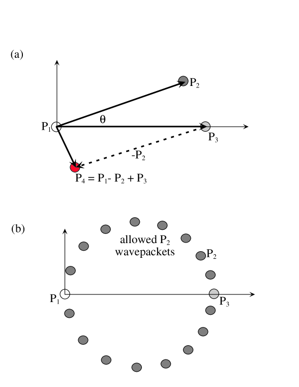
FIG. 1.: Momentum space view of the wavepackets participating in the four-wave mixing process. (a) Conservation of momentum in the laboratory frame. (b) A set of possible wavepackets in the laboratory frame with momenta that satisfy the phase-matching conditions in Section II C, namely, $|{\bf P}_{2}|=|{\bf P}_{3}|\cos{\theta}$.

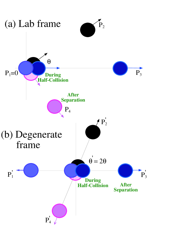
FIG. 2.: (a) Lab frame view of the four-wave mixing process, showing the four wavepackets at early time while they are still interacting and at late time after they have separated. (b) Degenerate frame view of the same cases as in (a).

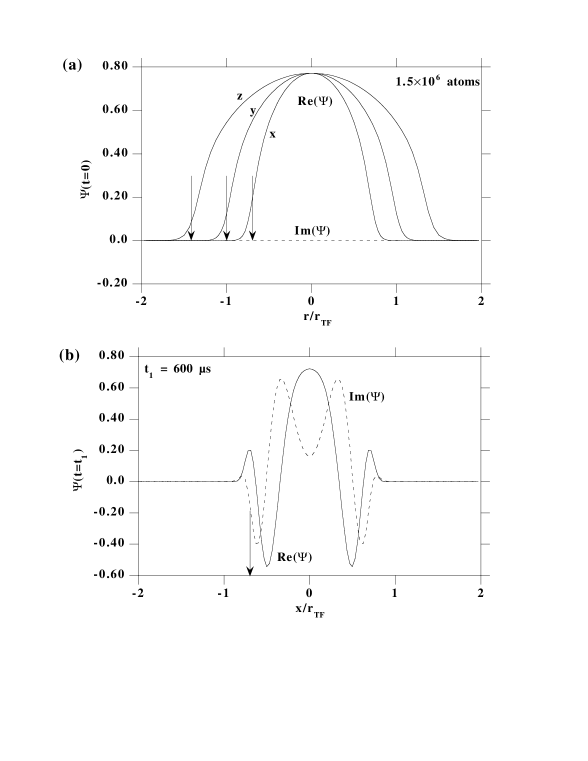
FIG. 3.: (a) Cuts along the $x$, $y$ and $z$ axes of the parent condensate wavefunction $\Psi(x,y,z,t=0)$ for $N=1.5\times 10^{6}$ atoms in a trap with harmonic frequencies of 84 Hz, 59.4 Hz, and 42 Hz in the respective $x$, $y$, and $z$ directions. The arrows show the TF radii $r_{TF}(i)$ in the $i=x,y,z$ directions. The curves labeled “$x$”, “$y$”, and “$z$” respectively represent $\mathrm{Re}[\Psi(x,0,0,0)]$, $\mathrm{Re}[\Psi(0,y,0,0)]$, and $\mathrm{Re}[\Psi(0,0,z,0)]$; $\mathrm{Im}[\Psi(x,y,z,0)]$ is identically zero for each case. (b) Cuts along the $x$ axis of $\mathrm{Re}[\Psi(x,0,0,t=t_{1})]$ and $\mathrm{Im}[\Psi(x,0,0,t=t_{1})]$ for $t_{1}=600\ \mu$s.

FIG. 4.: Cut in the $k_{x}$ direction $(k_{y}=k_{z}=0)$ of the squared momentum distribution $|\Psi({\bf k},t)|^{2}$ for the wavefunctions in Fig. 3 for $t_{1}=0$ and $t_{1}=600$ $\mu$s.

FIG. 5.: Comparison of $N_{4}(t)/N$ versus $t-t_{2}$ for 2D and 3D calculations for $1.5\times 10^{6}$ atoms. The trap is the same as in Fig. 3. The Bragg pulses are applied 600 $\mu$s after the trapping potential is turned off and are over at time $t_{2}$.

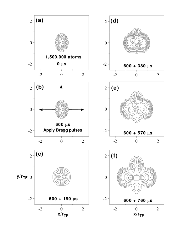
FIG. 6.: Contour plots of integrated column density from the 3D-SVEA calculations vs $x$ and $y$ for $N=1.5\times 10^{6}$ and the same trap as for Fig. 3. Panels (a) through (f) show the time development of the wavepackets from the from the time the trap is turned off until the wavepackets physically separate.

FIG. 7.: Comparison of $N_{4}(t)/N$ versus $t-t_{2}$ for $0.2\times 10^{6}$, $1.5\times 10^{6}$ and $5.0\times 10^{6}$ atoms. The trap is the same as in Fig. 3. The Bragg pulses are applied 600 $\mu$s after the trapping potential is turned off.

FIG. 8.: Comparison of $N_{4}(t)/N$ versus $t-t_{2}$ for $1.5\times 10^{6}$ atoms. The different curves show cases where the Bragg pulses are applied at $t_{1}=0$, $600$, $1200$ and $1800$ $\mu$s after the trapping potential is turned off ($t_{2}\approx t_{1}$). The trap is the same as in Fig. 3.

FIG. 9.: Comparison of $N_{4}(t)/N$ versus $t-t_{2}$ for $1.5\times 10^{6}$ atoms. The trap is the same as in Fig. 3. The Bragg pulses are applied 600 $\mu$s after the trapping potential is turned off. The three different curves are for the cases where the separation times are scaled by factors of 0.7, 1, and 2 by scaling the separation velocities by $1/0.7$, 1, and $1/2$.

FIG. 10.: Growth of $N_{4}(t)/N$ and $N_{4}(t)/N$ versus $t-t_{2}$ for the case where a weak probe wavepacket 2 with initial population fraction 0.001 encounters strong “pump” wavepackets with initial fractions 0.4995. The trap is the same as in Fig. 3. The Bragg pulses are applied 600 $\mu$s after the trapping potential is turned off.

FIG. 11.: $N_{4}/N$ dependence dependence on the total number of atoms, $N$, calculated in 2D and 3D. The dashed lines show the $N^{6/5}$ dependence predicted by the simple theory in subsection II D. The trap is the same as in Fig. 3. The Bragg pulses are applied 600 $\mu$s after the trapping potential is turned off.

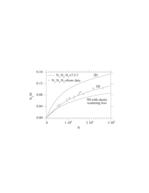
FIG. 12.: Fraction of atoms in the 4WM output wavepacket, $N_{4}/N$, versus the total number of initial atoms, $N$, calculated in 2D, 3D and 3D with inclusion of elastic scattering loss as discussed in Sec. II E. The open circles represent calculations using experimental data [2] to determine the ratios $N_{1}:N_{2}:N_{3}$ rather than taking the nominal values $N_{1}:N_{2}:N_{3}=7:3:7$. The trap is the same as in Fig. 3. The Bragg pulses are applied 600 $\mu$s after the trapping potential is turned off.

FIG. 13.: Fraction of atoms in the 4WM output wavepacket, $N_{4}/N$, versus the total number of initial atoms, $N$, calculated in 3D without and with inclusion of elastic scattering loss as discussed in Sec. II E. The dots are experimental data [2]. The trap is the same as in Fig. 3. The Bragg pulses are applied 600 $\mu$s after the trapping potential is turned off.

- [1] M. Trippenbach, Y. B. Band, and P. S. Julienne, Optics Express 3, 530 (1998).
- [2] L. Deng, E. W. Hagley, J. Wen, M. Trippenbach, Y. B. Band, P. S. Julienne, J.E. Simsarian, K. Helmerson, S.L. Rolston, and W.D. Phillips, Nature (London) 398, 218 (1999).
- [3] M.H. Anderson et al., Science 269, 198 (1995); K. B. Davis et al., Phys. Rev. Lett. 75, 3969 (1995); C.C. Bradley, et al., Phys. Rev. Lett. 78, 985 (1997); see also C.C. Bradley et al., Phys. Rev. Lett. 75, 1687 (1995).
- [4] See reviews of BEC by F. Dalfovo, S. Giorgini, L. P. Pitaevskii and S. Stringari, Rev. of Mod. Phys. 71, 463 (1999) and A. S. Parkins and D. F. Walls, Phys. Reports 303, 1 (1998).
- [5] M. O. Mewes, et al., Phys. Rev. Lett. 78, 582 (1997); B. P. Anderson and M A Kasevich, Science 282, 1686 (1998); E Hagley et al., Science 283, 1706 (1999); I. Bloch, T. W. Hänsch and T. Esslinger, Phys. Rev. Lett. 82, 3008 (1999).
- [6] M. Kozuma, L. Deng, E. W. Hagley, J. Wen, R. Lutwak, K. Helmerson, S. L. Rolston, and W. D. Phillips, Phys. Rev. Lett. 82, 871 (1999).
- [7] G. Lenz, P. Meystre and E.W. Wright, Phys. Rev. Lett. 71, 3271 (1993).
- [8] E. Goldstein, K. Plättner, and P. Meystre, Quantum Semiclass. Opt. 7, 743 (1995); E. Goldstein, K. Plättner, and P. Meystre, J. Res. Nat. Inst. Stand. Technol. 101, 583 (1996)
- [9] E. Goldstein and P. Meystre, Phys. Rev. A 59, 1509 (1999).
- [10] C. K. Law, H. Pu, and N. P. Bigelow, Phys. Rev. Lett. 81, 5257 (1998).
- [11] E. Goldstein and P. Meystre, Phys. Rev. A 59, 3896 (1999).
- [12] R. W. Hellwarth, Prog. Quant. Electr. 5, 1 (1977).
- [13] P. D. Maker and R. W. Terhune, Phys. Rev. A137, 801 (1965).
- [14] A. Yariv and D. M. Pepper, Opt. Lett. 1, 16 (1977).
- [15] M. Doery, private communication (1999).
- [16] R. J. Ballagh, K. Burnett and T. F. Scott, Phys. Rev. Lett. 78, 3276-3279 (1997).
- [17] H. Wallis, A. Rohrl, M. Naraschewski and A. Schenzle, Phys. Rev. A55, 2109 (1997).
- [18] M. Trippenbach and Y. B. Band, Phys. Rev. A56, 4242 (1997)
- [19] M. Trippenbach and Y. B. Band, Phys. Rev. A57, 4791 (1998).
- [20] Y. B. Band, M. Trippenbach, J. P. Burke, and P. S. Julienne, “Elastic scattering loss of atoms from colliding Bose-Einstein condensate wavepackets”, Phys. Rev. Lett. (submitted).
- [21] A.P. Chikkatur, A. Goerlitz, D.M. Stamper-Kurn, S. Gupta, S. Inouye, D.E. Pritchard, and W. Ketterle, to be published.
- [22] E. Tiesinga, C. J. Williams, P. S. Julienne, K. M Jones, P. D. Lett, and W. D. Phillips, J. Res. Natl. Inst. Stand. Technol. 101, 505 (1996).
- [23] J. A. Fleck, J. R. Morris and M. D. Feit, Appl. Opt. 10, 129 (1976); M. D. Feit and J. A. Fleck, Appl. Opt.17, 3390 (1978); Appl. Opt. 18, 2843 (1979).
- [24] Y. Castin and R. Dum,Phys. Rev. Lett 77, 5315 (1996).
- [25] Y. B. Band, Phys. Rev. A42, 5530 (1990).
- [26] Y. B. Band, E. Tiesinga, J. P. Burke, and P. S. Julienne, unpublished (2000).