Pulse driven switching in one-dimensional nonlinear photonic band gap materials: a numerical study

I INTRODUCTION

Nonlinear dielectric materials [2] exhibiting a bistable response to intense radiation are key elements for an all-optical digital technology. For certain input optical powers there may exist two distinct transmission branches forming a hysteresis loop, which incorporates a history dependence in the system’s response. Exciting applications involve optical switches, logic gates, set-reset fast memory elements etc [3]. Much interest has been given lately to periodic nonlinear structures [4], in which because of the distributed feedback mechanism, the nonlinear effect is greatly enhanced. In the low intensity limit, these structures are just Bragg reflectors characterized by high transmission bands separated by photonic band gaps [5]. For high intensities and frequencies inside the transmission band, bistability results from the modulation of transmission by an intensity-dependent phase shift. For frequencies inside the gap bistability originates from gap soliton formation [6], which can lead to much lower switching thresholds [7].

The response of nonlinear periodic structures illuminated by a constant wave (CW) with a frequency inside the photonic gap is generally separated into three regimes: i) steady state response via stationary gap soliton formation, ii) self-pulsing via excitation of solitary waves, and iii) chaotic. Much theoretical work has been done for systems with a weak sinusoidal refractive index modulation and uniform nonlinearity [4, 8, 9, 10, 11], or deep modulation multilayered systems [6, 12, 13], as well as experimental [14, 15]. One case of interest is when the system is illuminated by a CW bias and switching between different transmission states is achieved by means of external pulses. Such switching has already been demonstrated experimentally for various kinds of nonlinearities [14, 16, 17], but to our knowledge, a detailed study of the dynamics, the optimal pulse parameters and the stability under phase variations during injection, has yet to be performed.

In this paper we use the Finite-Difference-Time-Domain (FDTD) [18] method to study the time-dependent properties of CW propagation in multilayer structures with a Kerr type nonlinearity. We find our results generally in accord to those obtained for systems with weak linear index modulation [9], which were solved with approximate methods. We next examine the dynamics of driving the system from one transmission state to the other by injecting a pulse, and try to find the optimal pulse parameters for this switching. We also test how these parameters change for a different initial phase or frequency of the pulse. Finally, we will repeat all work for the case of a linear multilayer structure with a nonlinear impurity layer.

II FORMULATION

Electromagnetic wave propagation in dielectric media is governed by Maxwell’s equations

$$\mu\frac{\partial\vec{H}}{\partial t}=-\vec{\nabla}\times\vec{E} \frac{\partial\vec{D}}{\partial t}=\vec{\nabla}\times\vec{H}$$ (1)

Assuming here a Kerr type saturable nonlinearity and an isotropic medium, the electric flux density $\vec{D}$ is related to the electric field $\vec{E}$ by

$$\vec{D}=\epsilon_{0}\vec{E}+\vec{P}_{L}+\vec{P}_{NL}=\epsilon_{0}\left(\epsilon_{r}+\frac{\alpha|\vec{E}|^{2}}{1+\gamma|\vec{E}|^{2}}\right)\vec{E}$$ (2)

where $\gamma\geq 0$. $\vec{P}_{L}$ and $\vec{P}_{NL}$ are the induced linear and nonlinear electric polarizations respectively. Here we will assume zero linear dispersion and so a frequency independent $\epsilon_{r}$. Inverting this to obtain $\vec{E}$ from $\vec{D}$ involves the solution of a cubic equation in $|\vec{E}|$. For $\alpha\geq 0$ there is always only one real root, so there is no ambiguity. For $\alpha<0$ this is true only for $\gamma>0$. In our study we will use $\alpha=-1$ and $\gamma=(\epsilon_{r}-1)^{-1}$ so that for $|\vec{E}|\rightarrow\infty$, $\vec{D}\rightarrow\epsilon_{0}\vec{E}$.

The structure we are considering consists of a periodic array of 21 nonlinear dielectric layers in vacuum, each 20 nm wide with $\epsilon_{r}=3.5$, separated by a lattice constant $a=$200 nm. The linear, or low intensity, transmission coefficient as a function of frequency is shown in Fig. 1a. In the numerical setting each unit cell is divided into 256 grids, half of them defining the highly refractive nonlinear layer. For the midgap frequency, this corresponds to about 316 grids per wavelength in the vacuum area and 1520 grids per effective wavelength in the nonlinear dielectric, where of course the length scale is different in the two regions. Stability considerations only require more than 20 grids per wavelength [18]. Varying the number of the grids used we found our results to be completely converged. On the two sides of the system we apply absorbing boundary conditions [18].

We first study the structure’s response to an incoming constant plane wave of frequency close to the gap edge $\omega a/2\pi c=0.407$. For each value of the amplitude, we wait until the system reaches a steady state and then calculate the corresponding transmission and reflection coefficients. If no steady state is achievable, we approximate them by averaging the energy transmitted and reflected over a certain period of time, always checking that energy conservation is satisfied. Then the incident amplitude is increased to its next value, which is done adiabatically over a time period of 20 wave cycles, and measurements are repeated. This procedure continues until a desired maximum value is reached, and then start decreasing the amplitude, repeating backwards the same routine. The form of the incident CW is

$$E_{{CW}}(t)=\left(A_{{CW}}+dA_{{CW}}\frac{min\{(t-t_{0}),20T\}}{20T}\right)e^{i\omega t}$$ (3)

where $t_{0}$ is the time when the amplitude change started, $A_{{CW}}$ is the last amplitude value considered and $dA_{{CW}}$ the amplitude increment. One wave cycle $T$ involves about 2000 time steps.

III RESPONSE TO A CW BIAS

The amplitude of the CW is varied from zero to a maximum of 0.7 with about 40 measurements in between. Results are shown in Fig. 1b, along with the corresponding one from a time-independent approximation. The agreement between the two methods is exact for small intensities, however, after a certain input the output waves are not constant any more but pulsative. This is in accord with the results obtained with the slowly varying envelope approximation for systems with a weak refractive index modulation [9]. It is interesting that the averaged output power is still in agreement with the time-independent results, something not mentioned in earlier work. For higher input values, the solution will again reach a steady state just before going to the second nonlinear jump, after which it will again become pulsative. This time though, the averaged transmitted power is quantitatively different from the one predicted from time-independent calculations.

The nonlinear transmission jump originates from the excitation of a stationary gap soliton when the incident intensity exceeds a certain threshold value. Due to the nonlinear change of the dielectric constant, the photonic gap is shifted locally in the area underneath the soliton, which becomes effectively transparent, resembling a quantum well with the soliton being its bound state solution [19]. The incident radiation coupled to that soliton tunnels through the structure and large transmission is achieved. We obtain a maximum switching time of the order of 100 $T_{r}$, or a frequency of 360 GHz, where $T_{r}=2L/c$ is roundtrip time in vacuum. The second transmission jump is related to the excitation of two gap solitons, which however, are not stable and so transmission is pulsative. The Fourier transform of the output shows that, after the second transmission jump, the system pulsates at a frequency $\omega a/2\pi c=0.407\pm n\times 0.024$, exactly three times the one of the first pulsating solution $\omega a/2\pi c=0.407\pm n\times 0.008$, where $n$ is an integer. For much higher input values the response eventually becomes chaotic. A more detailed description of the switching process as well as the soliton generation dynamics can be found in [9].

IV PULSE DRIVEN SWITCHING

We next turn to the basic objective of this work. We assume a specific constant input amplitude $|A_{{CW}}|=0.185$ corresponding to the middle of the first bistable loop. Depending on the system’s history, it can be either in the low transmission state I, shown in Fig. 1c, or in the high transmission state II, shown in Fig. 1d, which are both steady states. We want to study the dynamics of a pulse injected into a system like that. More specifically, if it will drive the system to switch from one state to the other, how the fields change in the structure during switching, for which pulse parameters this will happen and if these parameters change for small phase and frequency fluctuations. We assume Gaussian envelope pulses

$$E_{{P}}(0,t)=A_{{P}}e^{-(t-t_{0}-5t_{w})^{2}/t_{w}^{2}}e^{i\omega t}$$ (4)

where $A_{{P}}$ is the pulse amplitude, $t_{0}$ the time when injection starts, and $W=2t_{w}c$ is the pulse’s full width at $1/e$ of maximum amplitude. The beginning of time $t$ is the same as for the CW, so there is no phase difference between them. After injection we wait until the system reaches a steady state again and then measure the transmission and reflection coefficients to determine the final state. During this time we save the field values inside the structure every few time steps, as well as the transmitted and reflected waves. This procedure is repeated for various values of $A_{{P}}$ and $t_{w}$, for both possible initial states. Our results are summarized in Fig. 2. White areas indicate the pulse parameters for which the intended switch was successful while black are for which it failed. In Fig. 2a, or the “Switch” graph, the intended switching scheme is for the same pulse to be able to drive the system from state I to state II and vise versa. Fig. 2b, or “Switch All Up”, is for a pulse able to drive the system from I to II, but fails to do the opposite, ie. the final state is always II independently from which the initial state was. Similarly, Fig. 2c or “Switch All Down”, is for the pulse whose final state is always I, and Fig. 2d or ”No Switch”, for the pulse that does not induce any switch for any initial state.

We find a rich structure on these parameter planes. Note also that there is a specific cyclic order as one crosses the curves moving to higher pulse energies: $\rightarrow$ d $\rightarrow$ b $\rightarrow$ a $\rightarrow$ c $\rightarrow$ etc. This indicates that there must be some kind of energy requirements for each desired switching scheme. After analyzing the curves it was found that only the first one in the “Switch” graph could be assigned to a simple constant energy curve $\mathcal{E}$$\sim W|A_{p}|^{2}$. Since any switching involves the creation or destraction of a stationary soliton, then this should be its energy. In order to put some numbers, if we would assume a nonlinearity $|\alpha|=10^{-9}$ cm²/W, then we would need a CW of energy $\simeq 34$ MW/cm² and a pulse of width $W/c$ of a few tenths of femtoseconds and energy $\mathcal{E}$$\simeq 2.5\mu$J/cm². These energies may seem large, but they can be sufficiently lowered by increasing the number of layers and using an incident frequency closer the the gap edge.

In order to find more about how the switching occurs, we plotted in Fig. 3 the effective transparent areas and the output fields as a function of time, for the first three curves of Fig. 2a. As expected, for the pulse from the first curve, the energy for the soliton excitation is just right, and the output fields are small compared to the input. For the other curves however, there is an excess of energy. The system has to radiate this energy away before a stable gap soliton can be created. It is interesting to note that this energy goes only in the transmitted wave, not the reflected, and it consists of a series of pulses [15]. For the second curve in Fig. 2a there is one pulse, for the third there are two etc. The width and frequency of the pulses are independent of the incident pulse, they are the known pulsating solutions we found in the CW case. So the system temporally goes into a pulsating state to radiate away the energy excess before settling down into a stable state. If this energy excess is approximately equal to an integer number of pulses (the solitary waves from the unstable solutions), then we will have a successful switch, otherwise it will fail. A similar behavior is found in the system’s response during switch down for the first three curves in Fig. 2a, using exactly the same pulses as before for the switch up. So the same pulse is capable of switching the system up, and if reused, switching the system back down. Using the numbers assumed before for the nonlinearity $\alpha$, the pulses used in Fig. 3 are (a) $W/c=14$ fs, $\mathcal{E}$=2.5 $\mu$J/cm², (b) $W/c=28$ fs, $\mathcal{E}$=12 $\mu$J/cm², (c) $W/c=42$ fs, $\mathcal{E}$=32 $\mu$J/cm².

Up to now, the injected pulse has been treated only as an amplitude modulation of the CW source, ie. they had the same exactly frequency and there was no phase difference between them. The naturally rising question is how an initial random phase between the CW and the pulse, or a slightly different frequency affect our results. We repeated the simulations for various values of an initial phase difference, first keeping them with the same frequency. We find that although the results show qualitatively the same stripped structure as in Fig. 2, there are quantitative differences. The main result is that there is not a set of pulse parameters that would perform the desired switching successfully for any initial phase difference. Thus the pulse can not be incoherent with the CW, ie. generated at different sources, if a controlled and reproducible switching mechanism is desired, but rather it should be introduced as an amplitude modulation of the CW. However, if this phase could be controlled, then the switching operation would be controlled, and a single pulse would be able to perform all different operations.

The picture does not change if we use pulses of slightly different frequency from the source. We used various pulses with frequencies both higher and lower than the CW, and we found a sensitive, rather chaotic, dependence on the initial phase at injection time. The origin of this complex response, if it is an artifact of the simple Kerr-type nonlinearity model that we used, and if it should appear for other kinds of nonlinearities, is not yet clear to as. More work is also needed on how these results would change if one used a different $|A_{{CW}}|$ not in the middle of the bistable loop, a wider or narrower bistable loop etc., but these would go more into the scope of engineering.

V LINEAR LATTICE WITH A NONLINEAR IMPURITY LAYER

Besides increasing the number of layers to achieve lower switching thresholds, one can use a periodic array of linear layers $\epsilon=\epsilon_{0}\epsilon_{r}$ with a nonlinear impurity layer [20, 21, 22, 23] $\epsilon=\epsilon_{0}(\epsilon_{r}^{\prime}+\alpha|\vec{E}|^{2})$ where $\epsilon_{r}\neq\epsilon_{r}^{\prime}$ and we will use $\alpha=+1$ and $\gamma=0$. This system is effectively a Fabry-Perot cavity with the impurity (cavity) mode inside the photonic gap, as shown in Fig. 4a. The bistable response originates from its nonlinear modulation with light intensity. The deeper this mode is in the gap, the stronger the linear dispersion for frequencies close to it. Because of the high $Q$ of the mode, we can use frequencies extremely close to it achieving very low switching thresholds [23]. Here however we only want to study the switching mechanism, so we will use a shallow impurity mode.

The bistable input-output diagram, the output fields during switching and the field distributions in the two transmission branches are also shown in Fig. 4. We observe a smaller relaxation time and of course the absence of pulsating solutions. The parameters used are $\epsilon_{r}^{\prime}=1$ and $\omega a/2\pi c=0.407$ which corresponds to a frequency between the mode and the gap edge. We want to test if a pulse can drive this system in switching between the two different transmission states, and again test our results against phase and frequency perturbations. The two states shown in Fig. 4 are for an input CW amplitude of $|A_{{CW}}|=0.16$. The results for coherent, pulse and CW, are shown in Fig.5. We see that any desired form of switching can still be achieved, but the parameter plane graphs no more bare any simple explanations as the ones obtained for the nonlinear superlattice. Repeating the simulations for incoherent beams and different frequencies we obtain the same exactly results as before. Only phase-locked beams can produce controlled and reproducible switching.

VI CONCLUSIONS

We have studied the time-dependent switching properties of nonlinear dielectric multilayer systems for frequencies inside the photonic band gap of the corresponding linear structure. The system’s response is characterized by both stable and self-pulsing solutions. We examined the dynamics of driving the system between different transmission states by pulse injection, and found correlations between the pulse, the stationary gap soliton and the unstable solitary waves. A small dependence on the phase difference between the pulse and the CW is also found, requiring coherent beams for fully controlled and reproducible switching. Similar results are also found for the case of a linear periodic structure with a nonlinear impurity.

FIG. 1.: (a) The linear transmission diagram. The small arrow indicates the frequency we used in the nonlinear study. (b) The nonlinear response: closed/(open) circles correspond to steady states when increasing/(decreasing) the intensity and crosses/(open squares) correspond to self-pulsing states when increasing/(decreasing) the intensity. (c) Intensity configuration for low transmission state. (d) Intensity configuration for high transmission state.

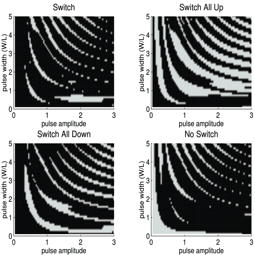
FIG. 2.: The four different switching schemes: (a) Final state opposite of initial, (b) final state always high transmission state, (c) final state always low transmission state, (d) no change of state. White areas indicate successful operation while black indicate failure.

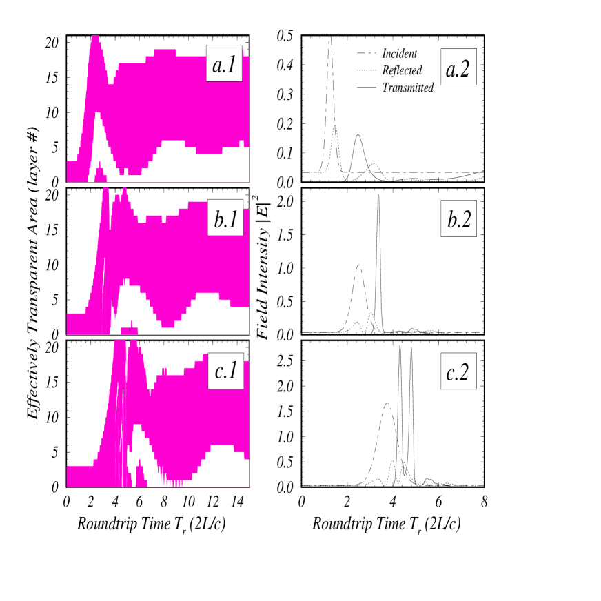
FIG. 3.: Switch-up dynamics for (a) First, (b) second and (c) third white curves in the “Switch” graph of Fig. 2. (1) Effectively transparent area and (2) input and output waves.

FIG. 4.: Linear lattice with a nonlinear impurity layer: (a) Linear transmission diagrams, (b) nonlinear response; solid/(open) circles for increasing/(decreasing) CW intensity, (c) output waves during switch-up and (d) switch-down, (e) intensity configuration for the low transmission state and (f) high transmission state.

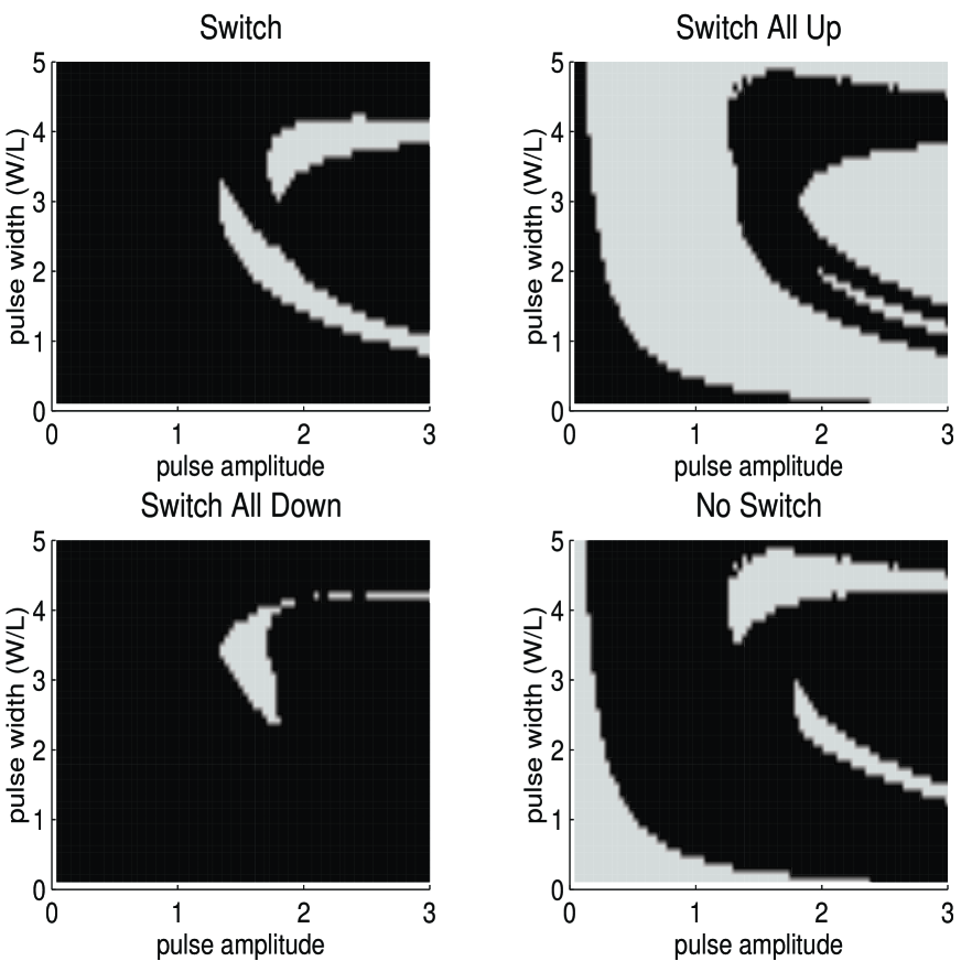
FIG. 5.: The four switching schemes described in Fig. 2 for the case of a linear lattice with a nonlinear impurity layer. No simple curved structure is found here.

- [1] Present address: Concurrent Computing Laboratory for Materials Simulation (CCLMS) and Department of Physics and Astronomy, Louisiana State University, Baton Rouge, LA 70803.
- [2] A. C. Newell and J. V. Moloney, Nonlinear Optics (Addison-Wesley, Redwood CA, 1992).
- [3] H. M. Gibbs, Optical Bistability: Controlling Light with Light (Academic, Orlando FL, 1985).
- [4] H. G. Winful, J. H. Marburger, and E. Garmire, Appl. Phys. Lett 35, 379 (1979); H. G. Winful, and G. D. Cooperman, Appl. Phys. Lett 40, 298 (1982).
- [5] Photonic Band Gaps and Localization, edited by C. M. Soukoulis (Plenum, New York, 1993); Photonic Band Gap Materials, edited by C. M. Soukoulis (Klumer, Dordrecht, 1996).
- [6] Wei Chen and D. L. Mills, Phys. Rev. B 36, 6269 (1987); Phys. Rev. Lett. 58, 160 (1987).
- [7] C. Martijn de Sterke and J. E. Sipe, in Progress in Optics, edited by E. Wolf (Elsevier, Amsterdam, 1994), Vol. 33.
- [8] D. L. Mills and S. E. Trullinger, Phys. Rev. B 36, 947 (1987).
- [9] C. Martijn de Sterke and J. E. Sipe, Phys. Rev. A 42, 2858 (1990).
- [10] A. B. Aceves, C. De Angelis and S. Wabnitz, Opt. Lett. 17, 1566 (1992).
- [11] Sajeev John and Neşet Aközbek, Phys. Rev. Lett. 71, 1168 (1993); Neşet Aközbek and Sajeev John, Phys. Rev. E 57, 2287 (1998).
- [12] Michael Scalora, Jonathan P. Dowling, Charles M. Bowden, and Mark J. Bloemer, Phys. Rev. Lett. 73, 1368 (1994).
- [13] P. Tran, Opt. Lett. 21, 1138 (1996).
- [14] N. D. Sankey, D. F. Prelewitz, and T. G. Brown, Appl. Phys. Lett. 60, 1427 (1992).
- [15] B. J. Eggleton, C. Martijn de Sterke, R. E. Slusher, J. Opt. Soc. Am. B 14, 2980 (1997).
- [16] S. S. Tarng, K. Tai, J. L. Jewell, H. M. Gibbs, A. C. Gossard, S. L. McCall, A. Passner, T. N. C. Venkatesan, W. Wiegmann, App. Phys. Lett. 40, 205 (1982).
- [17] J. He, M. Cada, M.-A. Dupertuis, D. Martin, F. Morier-Genoud, C. Rolland, A. J. SpringThorpe, Appl. Phys. Lett. 63, 866 (1993).
- [18] Allen Taflove, Computational Electrodynamics: The Finite-Difference Time-Domain Method (Artech House, Boston, 1995).
- [19] Elefterios Lidorikis, Qiming Li, and Costas M. Soukoulis, Phys. Rev. B 54, 10249 (1996).
- [20] Stojan Radic, Nicholas George, and Govind P. Agrawal, J. Opt. Soc. Am. B 12, 671 (1995).
- [21] Toshiaki Hattori, Noriaki Tsurumachi, and Hiroki Nakatsuka, J. Opt. Soc. Am. B 14, 348 (1997).
- [22] Rongzhou Wang, Jinming Dong, and D. Y. Xing, Phys. Rev. E 55, 6301 (1997).
- [23] E. Lidorikis, K. Busch, Qiming Li, C. T. Chan, and Costas M. Soukoulis, Phys. Rev. B 56, 15090 (1997).