Finite-time singularity in the dynamics
of the world population, economic and financial indices.
Running title: Finite-time singularity in world population growth

Abstract

Contrary to common belief, both the Earth’s human population and its economic output have grown faster than exponential, i.e., in a super-Malthusian mode, for most of the known history. These growth rates are compatible with a spontaneous singularity occuring at the same critical time $2052\pm 10$ signaling an abrupt transition to a new regime. The degree of abruptness can be infered from the fact that the maximum of the world population growth rate was reached in $1970$, i.e., about $80$ before the predicted singular time, corresponding to approximately $4\%$ of the studied time interval over which the acceleration is documented. This rounding-off of the finite-time singularity is probably due to a combination of well-known finite-size effects and friction and suggests that we have already entered the transition region to a new regime. In theoretical support, a multivariate analysis coupling population, capital, R&D and technology shows that a dramatic acceleration in the population during most of the timespan can occur even though the isolated dynamics do not exhibit it. Possible scenarios for the cross-over and the new regime are discussed.

Physica A 294 (3-4), 465-502 (15 May 2001)

1 Introduction

Both the world economy as well as the human population have grown at a tremendous pace especially during the last two centuries. It is estimated that 2000 years ago the population of the world was approximately 300 million and for a long time the world population did not grow significantly, since periods of growth were followed by periods of decline. It took more than 1600 years for the world population to double to 600 million and since then the growth has accelerated. It reached 1 billion in 1804 (204 years later), 2 billion in 1927 (123 years later), 3 billion in 1960 (33 years later), 4 billion in 1974 (14 years later), 5 billion in 1987 (13 years later) and 6 billion in 1999 (12 years later). This rapidly accelerating growth has raised sincere worries about its sustainability as well as concerns that we humans as a result might cause severe and irreversible damage to eco-systems, global weather systems etc [6, 22]. At, what one may say the other extreme, the optimists expect that the innovative spirit of mankind will be able to solve the problems associated with a continuing increase in the growth rate [15, 46]. Specifically, they believe that the world economic development will continue as a successive unfolding of revolutions, e.g., the Internet, bio-technological and other yet unknown innovations, replacing the prior agricultural, industrial, medical and information revolutions of the past. Irrespective of the interpretation, the important point is the presence of an acceleration in the growth rate. Here, it is first shown that, contrary to common belief, both the Earth human population as well as its economic output have grown faster that exponential for most of the known history and most strikingly so in the last centuries. Furthermore, we will show that both the population growth rate and the economic growth rate are consistent with a spontaneous singularity at the same critical time $2052\pm 10$ and with the same characteristic self-similar geometric patterns (defined below as log-periodic oscillations). Multivariate dynamical equations coupling population, capital and R&D and technology can indeed produce such an “explosion” in the population even though the isolated dynamics do not. In particular, this interplay provides an explanation of our finding of the same value of the critical time $t_{c}(\approx 2052\pm 10)$ both for the population and the economic indices. As a consequence, even the optimistic view has to be revised, since the acceleration of the growth rate contains endogenously its own limit in the shape of a finite-time singularity to be interpreted as a transition to a qualitatively new behaviour. Close to the mathematical singularity, finite-size effects will smoothen the transition and it is quite possible that Mankind may already have entered this transition phase. Possible scenarios for the cross-over and the new regime are discussed.

1.1 The logistic equation and finite-time singularities

As a standard model of population growth, Malthus’ model assumes that the size of a population increases by a fixed proportion $\tau$ over a given period of time independently of the size of the population and thus gives an exponential growth. The logistic equation attempts to correct for the resulting unbounded exponential growth by assuming a finite carrying capacity $K$ such that the population instead evolves according to

$${dp\over dt}=rp(t)\left[K-p(t)\right]~{}.$$ (1)

Cohen and others (see [6] and references therein) have put forward idealised models taking into account interaction between the human population $p(t)$ and the corresponding carrying capacity $K(t)$ by assuming that $K(t)$ increases with $p(t)$ due to technological progress such as the use of tools and fire, the development of agriculture, the use of fossil fuels, fertilisers etc. as well an expansion into new habitats and the removal of limiting factors by the development of vaccines, pesticides, antibiotics, etc. If $K(t)>p(t)$, then $p(t)$ explodes to infinity after a finite time creating a singularity. In this case, the limiting factor $-p(t)$ can be dropped out and, assuming a simple power law relationship $K\propto p^{\delta}$ with $\delta>1$, (1) becomes

$${dp\over dt}=r[p(t)]^{1+\delta}~{},$$ (2)

where the growth rate accelerates with time according to $r[p(t)]^{\delta}$. The generic consequence of a power law acceleration in the growth rate is the appearance of singularities in finite time:

$$p(t)\propto(t_{c}-t)^{z},~{}~{}{\rm with}~{}z=-{1\over\delta}~{}~{}\mbox{ and $t$ close to $t_{c}$}.$$ (3)

Equation (2) is said to have a “spontaneous” or “movable” singularity at the critical time $t_{c}$ [1], the critical time $t_{c}$ being determined by the constant of integration, i.e., the initial condition $p(t=0)$. One can get an intuitive understanding of such singularities by looking at the function $p(t)=\exp\left(tp(t)\right)$ which corresponds to replacing $\tau K$ by $p$ in Malthus’ exponential solution $p(t)=p(0)\exp[\tau Kt]$. $p$ is then the solution of $dp/dt=p^{2}/(1-tp)$ [1] leading to an ever increasing growth with the explicit solution

$$p(t)=e\left(1-C\sqrt{t_{c}-t}\right)~{},$$ (4)

where $t_{c}=1/e=0.368$, $C$ is a numerical factor and the exponent $z=1/2$. In this case, the finite time spontaneous singularity does not lead to a divergence of the population at the critical time $t_{c}$; only the growth rate diverges at $(t_{c}-t)^{-1/2}$. Spontaneous singularities in ODE’s and PDE’s are quite common and have been found in many well-established models of natural systems either at special points in space such as in the Euler equations of inviscid fluids [37] or in the equations of General Relativity coupled to a mass field leading to the formation of black holes [5], in models of micro-organisms aggregating to form fruiting bodies [39], or to the more prosaic rotating coin (Euler’s disk) [36], see [48] for a review. Some of the most prominent, as well as more controversial, examples due to their impact on human society are models of rupture and material failure [24, 28], earthquakes [29] and stock market crashes [26, 31].

1.2 Data sets and methodology

Here, we examine several data sets expressing the development of mankind on Earth in term of size and economic impact, to test the hypothesis that our history might be compatible with a future finite-time singularity. These data sets are as follows.

• The human population data from 0 to 1998 was retrieved from the web-site of The United Nations Population Division Department of Economic and Social Affairs (http://www.popin.org/pop1998/).

• The GDP of the world from 0 to 1998, estimated by J. Bradford DeLong at the Department of Economics, U.C. Berkeley [2], was given to us by R. Hanson [21].

• The financial data series include the Dow Jones index from 1790 [50] to 2000, the Standard & Poor (S&P) index from 1871 to 2000, as well as a number of regional and global indices since 1920. The Dow Jones index was constructed by The Foundation for the Study of Cycles [17]. It is the Dow Jones index back to 1896, which has been extrapolated back to 1790 and further. The other indices are from Global Financial Data [19]. These indices are constructed as follows. For the S&P, the data from 1871 to 1918 are from the Cowles commission, which back-calculated the data using the Commercial and Financial Chronicle. From 1918, the data is the Standard and Poor’s Composite index (S&P) of stocks. The other indices uses Global Financial Data’s indices from 1919 through 1969 and Morgan Stanley Capital International’s indices from 1970 through 2000. The EAFE Index includes Europe, Australia and the Far East. The Latin America Index includes Argentina, Brazil, Chile, Colombia, Mexico, Peru and Venezuela.

Demographers usually construct population projections in a disaggregated manner, filtering the data by age, stage of development, region, etc. Disaggregating and controlling for such variables are thought to be crucial for demographic development and for any reliable population prediction. Here, we propose a different strategy based on aggregated data, which is justified by the following concept: in order to get a meaningful prediction at an aggregate level, it is often more relevant to study aggregate variables than “local” variables that can miss the whole picture in favor of special idiosyncrasies. To take an example from material sciences, the prediction of the failure of heterogeneous materials subjected to stress can be performed according to two methodologies. Material scientists often analyse in exquisite details the wave forms of the acoustic emissions or other signatures of damage resulting from micro-cracking within the material. However, this is of very little help to predict the overall failure which is often a cooperative global phenomenon [23] resulting from the interactions and interplay between the many different micro-cracks nucleating, growing and fusing within the materials. In this example, it has been shown indeed that aggregating all the acoustic emissions in a single aggregated variable is much better for prediction purpose [28].

1.3 Content of the paper

In the next section, we first show that the exponential model is utterly inadequate in describing the population growth as well as the growth in the World GDP and the global and regional financial indices. We then present the alternative model consisting of a power law growth ending at a critical time $t_{c}$. We first give a non-parametric approach complemented by a fitting procedure. Section 3 proposes a first generalization of power laws with complex exponents, leading to so-called log-periodic oscillations decorating the overall power law acceleration. The fitting procedure is described as well as a non-parametric test of the existence of the log-periodic patterns for the world population. Section 4 presents a second-order generalization of the power law model, which allows for a frequency modulation in the log-periodic structure. This extended formula is used to fit the extended Dow Jones Industrial average. Section 5 summarizes what has been achieved and compares our results with previous work. In particular, we give the explicit solutions of multivariate dynamical equations for several coupled variables, such as population, technology and capital, to show that the same finite-time singularity can emerge from the interplay of these factors while each of them individually is not enough to create the singularity. Section 6 concludes by discussing a set of scenarios for mankind close to and beyond the critical time.

2 Singular Growth Rate

2.1 Tests of exponential growth

2.1.1 Human population and world GDP

A faster than exponential growth is clearly observed in the human population data from year 0 up to 1970, at which the estimated annual rate of increase of the global population reached its (preliminary?) all-time peak of $2.1\%$. Figure 4 shows the logarithm of the estimated world population as a function of (linear) time, such that an exponential growth rate would be qualified by a linear increase. In contrast, one clearly observes a strong upward curvature characterising a “super-exponential” behaviour. A faster than exponential growth is also clearly observed in the estimated GDP (Gross Domestic Product) of the World, shown in figure 4 for the year 0 up to 2000.

2.1.2 Financial indices

Over a shorter time period, a faster than exponential growth is also observed in figures 4 to 8 for a number of economic indicators such as the Dow Jones Average since the establishment of the U.S.A. in 1790 [50], the S&P since 1871, as well for a number of regional and global indices since 1920, including the Latin American index, the European index, the EAFE index and the World index. In all these figures, the logarithm of the index is plotted as a function of (linear) time, such that an exponential growth rate would be qualified by a linear increase. In all cases, one clearly observes in contrast a significant upward curvature characterising a “super-exponential” behaviour.

2.2 A first test of power law growth

2.2.1 Procedure

As shown in the derivation of equation (2), it is enough that the growth rate increases with any arbitrarily small positive power of $p(t)$ for a finite-time singularity to develop with the characteristic power law dependence (3). Can such a behaviour explain the super-exponential behaviour documented in the figures 4-8?

The small number of data points in these time series and the presence of large fluctuations prevent the use of a direct fitting procedure with (3). Indeed, such a fit, which typically attempts to minimise the root-mean-square (r.m.s.) difference between the theoretical formula and the data, is highly degenerate: many solutions are found which differ by variations of at most a few percent of the root-mean-square (r.m.s.) of the errors. Such differences in r.m.s. are not significant, especially considering the strongly non-Gaussian nature of the fluctuations in these data sets. Maximum likelihood methods are similarly limited. To address this problem of degeneracy, we turn to a non-parametric approach, consisting in fixing $t_{c}$ and plotting the logarithm of the data as a function of $\log(t_{c}-t)$. In such a plot, a linear behaviour qualifies the power law (3), and the slope gives the exponent $z$ which then can be determined visually or, better, by a fit but now with $t_{c}$ fixed. This procedure is not plagued by the previously discussed degeneracy and provides reliable and unique results.

2.2.2 World population

In figures 12-12, the world population in logarithm scale is shown as a function of $t_{c}-t$ also in logarithmic scale for three choices 2030, 2040 and 2050, respectively for $t_{c}$. Even though the fits with equation (3) for three cases varies in quality, they all capture the acceleration in the second half of the data on a logarithmic scale. The curvature seen in the data far from $t_{c}$ can be modeled by including a constant term in equation (3) embodying for instance the effect of an initial condition, as we discuss below. Changing $t_{c}$ from 2030 to 2050 has two competing effects observed in figures 12-12: a larger value of $t_{c}$ provides a better fit in the latter time period while deteriorating somewhat the fit to the data in the early time periods.

2.2.3 World GDP

As discussed in the introduction, the human population is strongly coupled with its outputs and with the Earth’s carrying capacity, and can partly be measured by its economic production. Hence, we should expect a close relationship between the size of the human population and its GDP. Figures 12-16 show the logarithm of the estimated World GDP as a function of $t_{c}-t$, both in log-log coordinates, where $t_{c}$ has been chosen to 2040, 2050 and 2060, respectively. The equation (3) is again parameterising the data quite satisfactorily.

We stress that we use the logarithm of the World GDP as well as the logarithm of the national, regional or global indices presented below as the “bare” data on which we test the power law hypothesis. This means that we plot the logarithm of the GDP or of the indices in logarithmic scale, which effectively amounts to taking the logarithm of the logarithm of the GDP as a function of $t_{c}-t$, itself also in logarithmic scale in order to test for the power law (3). This is done in an attempt to minimise the effect of inflation and other systematic drifts, and in accordance with standard economic practice that only relative changes should be considered. Removing an average inflation of 4% does not change the results qualitatively but the corresponding results are not quantitatively reliable as the inflation has varied significantly over US history with quantitative impacts that are difficult to estimate.

2.2.4 Financial indices

Further support for a singular power law behaviour of the economy can be found by analysing in a similar way the national, regional or global indices shown in figures 4-8. The results are shown in figures 16-32. Equation (3) is again perfectly compatible with the data and much better than any exponential model. As shown in Table 1, the fits of all six indices are found to be consistent with similar values for the exponent $z\approx-1$, the absolute value of the exponent increasing with $t_{c}$.

The results presented in this section on the world population, on the world GDP and on six financial indices suggest that the power law (3) is an adequate model. It is also parsimonious since the same simple mathematical expression, approximately the same critical time $t_{c}$ and same exponent are found consistently for all time series. These results confirm and extend the analysis presented forty years earlier for the world population only [16], which concluded at a $t_{c}=2026$. The results shown in the figures 12-12, with the sensitivity analysis provided by varying $t_{c}$ from 2030 to 2050, illustrate the large uncertainty in its determination. It is thus worthwhile to attempt quantifying further the observed power law growth and test how well $t_{c}$ is constrained.

2.3 Quantitative fits to a power law

In the derivation of (3), a key assumption was to neglect the limiting negative term in (1), which is warranted sufficiently close to $t_{c}$. Far from $t_{c}$, this analysis and more general considerations lead us to expect the existence of corrections to the pure power law (3). Furthermore, it may be necessary to include higher order terms as well as generalise the exponent as we will see in the next section.

The simplest extension of equation (3) is

$$p(t)=A+B(t_{c}-t)^{z}~{}.$$ (5)

In order to make a first quantitative estimate of the acceleration in the growth rate, determined by the exponent $z$ and the position $t_{c}$ of the singularity, we now let $t_{c}$ be a free parameter. In figure 33, the equation (5) is fitted to the world population from 0 to 1998. The parameter values of the fit are $A\approx 0$, $B\approx 22120$, $t_{c}\approx 2078$ and $z\approx-1.9$. The negative value of the exponent is compatible with $A\approx 0$. The negative exponent $z\approx-1.9$ obtained in the fit means that equation (5) has a singularity at $t=t_{c}$ corresponding to an infinite population. This is clearly impossible on a finite Earth. The point to be extracted from this analysis is that the world population has until very recently grown at an accelerating growth rate in good agreement with a singular behaviour. Singularities are always mathematical idealisations of natural phenomena: they are not present in reality but foreshadow an important transition or change of regime. In the present context, they must be interpreted as a kind of “critical point” signaling a fundamental and abrupt change of regime similar to what occurs in phase transitions [20].

As already discussed in relation with equation (1) and in the previous section, the world population growth cannot be separated from that of its evolving carrying capacity. As a first attempt to quantify this variable in an independent way, we analyse quantitatively the two largest data sets among all the financial indices and GDP: due to the large fluctuations of the financial indices compared to the number of points, only the S&P and the Dow Jones Average gave reliable results when $t_{c}$ is a free parameter. Figure 34 shows the corresponding fits with equation (5). The parameter values of the best fits are $A\approx-14$, $B\approx 71$, $z\approx-0.27$ and $t_{c}\approx 2068$ for the Dow Jones Average and $A\approx 0$, $B\approx 1693$, $z\approx-1.3$ and $t_{c}\approx 2067$ for the S&P. The fit with equation (5) exemplifies the acceleration of the growth rate, which is our main message. However, the location of the critical point is still not very reliable when based on simple power fits of very noisy data [10]. This motivates us to extend this analyses in the following sections.

3 Beyond a simple power law

The results shown in the figures 12-32, with the sensitivity analysis provided by varying $t_{c}$ from 2030 or 2040 to 2050 or 2060, illustrate the large uncertainty in the determination of the critical time. The direct fit with (5) still gives a very large uncertainty. As can be seen from the figures, an important reason lies in the existence of large fluctuations around the average power law behaviour. In the next section, we will see that this variability might be genuine and not simply noise. Furthermore, adding an extra degree of freedom will certainly improve a parametrisation of the data.

3.1 Generalisation to power laws with complex exponents: log-periodicity

The idea is to generalise the real exponent $z$ to a complex exponent $\beta+i\omega$, such that a power law is changed into $(t_{c}-t)^{\beta+i\omega}$, whose real part is $(t_{c}-t)^{\beta}\cos\left(\omega\ln(t_{c}-t)\right)$ [48]. The cosine will decorate the average power law behaviour with so-called log-periodic oscillations, the name steming from the fact the oscillations are periodic in $\ln(t_{c}-t)$ and not in $t$. As we shall see, these log-periodic oscillations can account for a large part of the observed variability around the power law. Thus, taking them into account provides a better parametrisation of the data and hence better constraints on the parameters of the power law $\beta$ and $t_{c}$.

There are fundamental reasons for introducing log-periodic corrections. Singularities often exhibit genuine log-periodic corrections that result from specific mechanisms [48]: singularities in the Euler equations with complex exponents have been found to result from a cascade of Rayleigh-Taylor instabilities leading to log-periodic oscillatory structures around singular vortices organised according to discrete self-similar pancakes[37]; in the process of formation of black holes, the matter field solution oscillates periodically in the logarithm of the difference between time and time of the formation of the singularity [5]; the phase separation kinetics of a binary mixture subjected to an uniform shear flow quenched from a disordered to a homogeneous ordered phase exhibits log-periodic oscillations due to a cyclical mechanism of stretching and break-up of domains, which allows to store and dissipate elastic energy in the system [7]; material failure occurs after intermittent damage acceleration and quiescent phases that are well-described by log-periodic structures decorating an overall power law singularity [24]; stock market crashes preceded by speculative bubbles [26, 31] provide an highly relevant analogy to the question of sustainability in the growth rate of the human population. More generally, from the point of view of field theory as a tool-box for constructing theories of complex systems, we should expect generically the existence of complex exponents and their associated log-periodic corrections [43]. We suggest that the presence of log-periodic oscillations deriving from general theoretical considerations can provide a first step to account for the ubiquitous observation of cycles in population dynamics and in economics.

3.2 Log-periodic fit of the World population

3.2.1 Results

Guided by the recent progress in the understanding of complex systems and the possibility of complex exponents discussed in the previous section, we have also fitted the world population data with the following equation

$$p(t)\approx A_{1}+B_{1}(t_{c}-t)^{\beta}+C_{1}(t_{c}-t)^{\beta}\cos\left(\omega\ln(t_{c}-t)+\phi\right)~{},$$ (6)

as shown in figure 33. We obtained two solutions, the best having $A\approx 0$, $B\approx 1624$, $C\approx-127$, $z\approx-1.4$, $t_{c}\approx 2056$, $\omega\approx 6.3$ and $\phi\approx 5.1$. The second solution has $A\approx 0.25$, $B\approx 1624$, $C\approx-127$, $z\approx-1.7$, $t_{c}\approx 2079$, $\omega\approx 6.9$ and $\phi\approx-4.4$. In this extension of equation (5), the cosine term embodies a discrete scale invariance [12] decorating the overall acceleration with a geometrical scaling ratio $\lambda=\exp\left(2\pi/\omega\right)$: the local maxima of the oscillations are converging to $t_{c}$ with the geometrical ratio $1/\lambda$.

3.2.2 Sensitivity analysis

Due to the small number of points in the population data set, the robustness of the fit with equation (6) was investigated with respect to fluctuations in the important physical parameters $t_{c}$, $\beta$ and $\omega$ [14]. The method we used was as follows. Together with the data set (data set 1) obtained from the United Nations Population Division Department of Economic and Social Affairs (see the introduction section), which covers the period $\left[0:1998\right]$, seven other data sets where analysed in an identical manner. These first three data sets were generated by removing the first point (data set 2), the two first points (data set 3) and the 3 first points (data set 4). Hence, those three data sets cover the periods $\left[1000:1998\right]$, $\left[1250:1998\right]$ and $\left[1500:1998\right]$. A fifth data set (data set 5) was constructed by including the UN estimate that the world’s population would reach 6 billion in October 1999 to the original data set (data set 1). Three additional data sets were created by removing points in the other end from the original data set (data set 1), i.e, by removing the last point (data set 6), the two last points (data set 7) and the three last points (data set 8). Hence, those three data sets cover the periods $\left[0:1990\right]$, $\left[0:1980\right]$ and $\left[0:1970\right]$.

The differences between the results obtained for the first five data sets are minor, as can be seen in Table 2 showing the values corresponding to the best fits. Data set 6 and 7 are also compatible with the previous 5 whereas the fit to data set 8 exhibit a significant discrepancy. For $t_{c}$, this gives the window 2052 $\pm$ 10 years, which is rather well-constrained. Furthermore, the values obtained for $\omega\approx 6\pm 0.5$ (again except for data set 8) are also quite compatible with previous results. The corresponding fluctuations in the fundamental parameters $z\approx 1.35\pm 0.11$ and $\lambda\approx 2.8\pm 0.3$ are also within reasonable bounds. Note that it is difficult to obtain a better resolution in time as world population statistics in past centuries are all generated by using some sort of statistical regression model. This might explain the relatively low value of the spectral peak obtained for data set 5, see below. Furthermore, the peak clearly stands out against the background for seven out of eight spectra as we now discuss. Another encouraging observation is the notable amplitude of the log-periodic oscillations quantified by $C$, approximately $5-10\%$ of the pure power law acceleration quantified by $B$, as seen in the caption of figure 33.

3.2.3 Non-parametric tests of log-periodicity

We also present a non-parametric test for the existence of the log-periodic oscillations decorating the spontaneous singularity, obtained by eliminating the leading trend using the transformation

$$p\left(t\right)\rightarrow\frac{p\left(t\right)-A_{1}-B_{1}(t_{c}-t)^{\beta}}{C_{1}(t_{c}-t)^{\beta}}~{}.$$ (7)

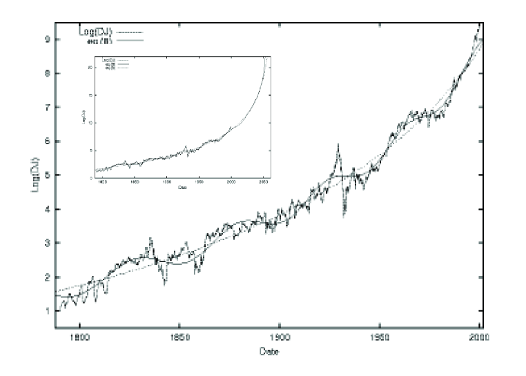
Figure 35: Left: Residue between best fit and data sets 3 and 5, as defined by equation $(\ref{residue})$. Right: Spectrum of residue using a Lomb periodogram. The position of the peak corresponds to $\omega\approx 5.8$, which should be compared with $\omega\approx 6.5$ for the fit with equation $(\ref{lppow})$ for data set 5. For data set 3, the peak corresponds to $\omega\approx 6.1$, which should be compared with $\omega\approx 6.5$ for the fit.

Figure 36: The circles are the logarithm of the yearly quotes from Dec. 1790 to Dec. 1999, which are shown instead of the monthly quotes used in the fit to better show the two fit curves. The upward trending full line is the best fit with equation $(\ref{eq:solution})$ with $\mbox{r.m.s.}=0.307$, $A\approx-13.7$, $B\approx 70.8$, $z\approx-0.27$ and $t_{c}\approx 2068$. The full oscillating line is the best fit with equation $(\ref{2feq})$ to the extended Dow Jones for the period $\left[1790:1999.75\right]$. The fit gives $\mbox{r.m.s}=0.236$, $A\approx 25.1$, $B\approx-4.13$, $C\approx-0.055$, $\beta\approx 0.39$, $t_{c}\approx 2053$, $\omega\approx 6.5$, $\tau\approx 171$, $\Delta\omega\approx-58$ and $\phi\approx-5.8$. The inset shows the extrapolation of the fit up to the critical time $t_{c}\approx 2053$.

This transformation should produce a pure $\cos\left(\omega\ln(t_{c}-t)+\phi\right)$ if equation (6) was a perfect description. In figure 36, we show the residual defined by (7) for data 3 and data 5 as a function of $\ln(t_{c}-t)$ as well as their Lomb periodograms which provide a power spectrum analysis for unevenly sampled data: the approximately regular oscillations in $\ln(t_{c}-t)$ give a significant spectral peak at a log-angular frequency $\omega\approx 5.8-6.1$ compatible with the fit of equation (6), see Table 2.

3.3 Summary

To sum up the evidence obtained so far, the comparison between the semi-logarithmic plots in figures 4-8 and the log-log plots in figures 12-32 validate the power law model (3) at the expense of the exponential model: there is no doubt that the world population and major economic and financial indices on average have grown much faster than exponentially. The second message is that the rather large fluctuations decorating an average power law acceleration can be remarkably well described by a simple generalisation of the power law in terms of a complex exponent: not only do we see a good agreement between the spectral analysis and the fits with equation (6), in addition the small fluctuations in the values for $t_{c}$, $\beta$ and $\omega$ for the 7 of the 8 data sets make the analysis credible for the world population. Of course, this does not prove that equation (6) is the correct description and equation (5) is a wrong description. However, since the r.m.s. of the fits with the two equations differs by a factor of $\approx 4$, there is no doubt that equation (6) does a better job of parameterising the data. This is the numerical argument. The theoretical justification has already been given above. The two combined certainly makes the case stronger. For the financial indices, the use of equation (6) does not lead to a significant improvement, and this leads us to examine the relevance of the next order of the expansion of corrections to the power law.

4 To second order

4.1 Next order of the log-periodic expansion

The data set containing the Dow Jones Average consists of $\approx 2500$ monthly quotes for the period $\left[1790:1999.9\right]$. We propose that it is representative of the capitalistic growth of the U.S.A. The time span and the sampling rate of this data set makes it reasonable to use the generalisation (12) of (6) to second order which allows for a continuous shift in the angular log-frequency $\omega$ [47] in what effectively corresponds to a Landau or renormalisation group expansion depending on the prefered framework.

We briefly summarize the method. Using the renormalization group (RG) formalism on a financial index $I$ amounts to assuming that the index at a given time $t$ is related to that at another time $t^{\prime}$ by the transformations

$$x^{\prime}=\phi(x)~{},$$ (8)

$$F(x)=g(x)+\frac{1}{\mu}F\biggl{(}\phi(x)\biggl{)}~{},$$ (9)

where $x=t_{c}-t$. $t_{c}$ is the critical time and $\phi$ is called the RG flow map. Here,

$$F(x)=I(t_{c})-I(t)~{},$$

such that $F=0$ at the critical point and $\mu$ is a constant describing the scaling of the index evolution upon a rescaling of time (8). The function $g(x)$ represents the non-singular part of the function $F(x)$. We assume as usual that the function $F(x)$ is continuous and that $\phi(x)$ is differentiable. In order to use this formalism to constrain the possible time dependence of the index, we notice that the solution in terms of a power law of the RG equation (9) together with (8) and the linear approximation $\phi(x)=\lambda x$ valid close to the critical point can be rewritten as

$${dF(x)\over d\ln x}=\alpha F(x)~{}.$$ (10)

This states simply that a power law is nothing but a linear relationship when expressed in the variables $\ln F(x)$ and $\ln x$. A critical point is characterized by observables which have an invariant description with respect to scale transformations on $x$. We can exploit this and the expression (10) to propose the structure of the leading corrections to the power law with log-periodicity. Hence, we notice that (10) can be interpreted as a bifurcation equation for the variable $F$ as a function of a fictitious “time” ($\ln x$) as a function of the “control parameter” $\alpha$. When $\alpha>0$, $F(x)$ increases with $\ln x$ while it decreases for $\alpha<0$. The special value $\alpha=0$ separating the two regimes corresponds to a bifurcation. Once we have recognized the structure of the expression (10) in terms of a bifurcation, we can use the general reduction theorem telling us that the structure of the equation for $F$ close to the bifurcation can only take a universal non-linear form given by

$${dF(x)\over d\ln x}=(\alpha+i\omega)F(x)+(\eta+i\kappa)|F(x)|^{2}+{\cal O}(F^{3}).$$ (11)

where $\alpha>0$, $\omega$, $\eta$ and $\kappa$ are real coefficients and ${\cal O}(F^{3})$ means that higher order terms are neglected. The generality of this expression stems from the fact that it is nothing but a Taylor’s expansion of a general functional form ${dF(x)\over d\ln x}={\cal F}(F(x))$. Such expansions are known in the physics literature as Landau expansions. We stress that this expression represents a non-trivial addition to the theory, constrained uniquely by symmetry laws. Going up to second order included, equation $(\ref{lppow})$ becomes [47]

$$\ln\left(I\left(t\right)\right)=A_{2}+B_{2}{\left(t_{c}-t\right)^{\beta}\over\sqrt{1+\left({t_{c}-t\over\tau}\right)^{2\beta}}}\left[1+C_{2}\cos\biggl{(}\omega\ln\left(t_{c}-t\right)+{\Delta\omega\over 2\beta}\ln\left(1+\left({t_{c}-t\over\tau}\right)^{2\beta}-\phi\right)\biggl{)}\right]~{}.$$ (12)

This extension has been found useful in order to account for the behaviour of stock market prices before large crashes over extended period of times up to 8 years. The present analysis thus constitutes a major generalisation as it includes over 200 years of data. Previous work have established a robust and universal signature preceding large crashes occuring in major financial stock markets, namely accelerated price increase decorated by large scale log-periodic oscillations culminating in a spontaneous singularity (critical point). The previously reported cases, which are well-described by equation $(\ref{lppow})$, comprise the Oct. 1929 US crash, the Oct. 1987 world market crash, the Jan. 1994 and Oct. 1997 Hong-Kong crashes, the Aug. 1998 global market event, the April 2000 Nasdaq crash, the 1985 Forex event on the US dollar, the correction on the US dollar against the Canadian dollar and the Japanese Yen starting in Aug. 1998, as well as the bubble on the Russian market and its ensuing collapse in June 1997 [26, 31]. Furthermore, twenty-one significant bubbles followed by large crashes or by severe corrections in the stock markets indices of the South American and Asian countries, which exhibit log-periodic signatures decorating an average power law acceleration, have also been identified [30]. In all these analyses, the time scales have been restricted to 1 to 8 years. In contrast, the general renormalisation group theory of such spontaneous singularities allow for an hierarchy of critical points at all scales [8, 44]. The results given below suggest that singularities do indeed cascade in a robust way up to the largest time scales or conversely from the largest scale to the smallest scales [11].

4.2 Second order fit of the Dow Jones Average index

4.2.1 Methodology

We fit the logarithm of the extended Dow Jones index to equation (12). As mentioned, taking the logarithm provides in our opinion the simplest and most robust way to account for inflation. Furthermore, taking the logarithm embodies the notion that only relative changes are important. Another more subtle reason can be given in terms of the magnitude of the crash following the singularity: a simple model of rational expectations [25] shows that if the loss during a crash is proportional to the maximum price, then the relevant quantity is the logarithm of the price in accordance with the standard economic notion that only relative changes should be relevant.

Fitting equation (12) to some data set is difficult even with a large data set (for noisy data with only a few hundred points or less, it becomes quite impossible), due to the degenerate r.m.s. landscape corresponding to the existence of many local minima as a function of the free parameters $t_{c}$, $\beta$, $\omega$, $\tau$ $\Delta\omega$ and $\phi$. This means that the r.m.s. alone is not a good measure of the quality of the fit and additional physical constraint are needed as discriminators. This has been discussed at length in [27]. In brief, we will demand that the value of $\beta$ and $\omega$ are compatible with what has been found previously for large crashes and that the value of the transition time $\tau$ between the two competing frequencies is compatible with the time window $t_{c}-t_{0}$, where $t_{0}$ is the date of the first data point and $t_{c}$ the date of the singularity in the first derivative. Unfortunately, we have no means to impose a criterion on the frequency-shift $\Delta\omega$.

Specifically, we will demand that $0.2<\beta<0.7$, $4.5<\omega<9$ and $\left(t_{c}-t_{0}\right)/3<\tau\stackrel{{\scriptstyle<}}{{\sim}}\left(t_{c}-t_{0}\right)$ and the more the parameters fall in the mid-range, the higher confidence is attributed to the fit. These constraints are similar to what was used in [27] except for the constrain on $\tau$ which upper limit has been made stricter here. The reason for this is simply that, whereas in the cases of the 1929 and 1987 stock market crashes on Wall Street, it was not obvious to decide the starting date of the bubble, it is now objectively determined by a historical event being the creation of the U.S.A. as an independent nation [50]. The parameter values of the five qualifying fits is shown in Table 3. We stress that the majority of the fits were discarded due to rather large values for either $\omega$ or $\tau$ or negative values for $\omega$. We see that the best fit in terms of the r.m.s. also has the most reasonable parameter values for $\beta$, $\omega$ and $\tau$ in terms of the discussion above.

4.2.2 Results

The best fit of equation (12)) to the $210$ years of monthly quotes is shown in figure 36 and its parameter values are given in the caption. Note that the value of the angular log-frequency $\omega\approx 6.5$ compared to $\omega\approx 6.3$ as well as the value for the position of the singularity $t_{c}\approx 2053$ compared $t_{c}\approx 2056$ are in close agreement with the values found for the analysis of the world population. Furthermore, the cross-over time scale $\tau\approx 171$ years is perfectly compatible with the total time window of 210 years. In figure 37, the relative error between the fit and the data is shown. We see that the error fluctuates nicely around zero as it should. Furthermore, the error is decreasing from left to right clearly showing that the acceleration in the data is better and better modeled by equation (12)) as we approach the present. This behaviour is in fact to be expected from an equation such as (2) allowing for an additive noise term to describe other sources of uncertainties: using the Fokker-Planck formalism, one can show that, as the singularity at $t_{c}$ is approached, the noise term becomes negligible and the acceleration of the data should approach better and better a pure power law. This can also be seen directly from (2) with an additive noise: the divergence of $p(t)$ dwarves any bound noise contribution.

4.2.3 Discussion

The inset of figure 36 shows the extrapolation of the fit up to the critical time $t_{c}=2053$. It suggests that the Dow Jones index will climb to impressive values in the coming decades from its present level around 11,000 at the beginning of year 2000. It is interesting that this resonates with a series of claims that the Dow Jones will climb to 36,000 [18], 40,000 [13] or even 100,000 [32] in the next two or three decades. Glassman, an investing columnist for the Washington Post, and Hassett, a former senior economist with the Federal Reserve, develop the argument that stocks have been undervalued for decades and that, for the next few years, investors can expect a dramatic one-time upward adjustment in stock prices [18]. Elias, a financial advisor and author, believes that forces such as direct foreign investment, domestic savings, and cooperative central-banking policies will drive the vigorous market, as will the dynamics of the New Economy, which allows for the coexistence of high economic growth, low interest rates, and low inflation. In his view, the Dow Jones could reach 40,000 around 2016 [13]. Kadlec, chief investment strategist for Seligman Advisors Inc. predicts that the Dow Jones Industrial Average will end up at 100,000 in the year 2020 [32]. We find that equation (12) predicts that the level 36,000-40,000 will be reached in 2018-2020 A.D. and the level 100,000 in 2026 A.D, not far from these claims! Of course, the extrapolation of this growth closer to the singularity becomes unreliable due to standard limitations, such as finite size effects, and must be taken with a “hand-full of salt”.

In the academic financial literature, a time series such as the Dow Jones shown in figure 36 has been argued to exhibit an anomalously large return, averaging $6\%$ per year over the 1889-1978 period [35], which cannot be explained by any reasonable risk aversion coefficient. A solution for this puzzle is that infrequent large crashes occur or even a major still untriggered crash is looming over us; in this interpretation, the “anomalous” return becomes the normal remuneration for the risk to stay invested in the market [40]. Our analysis suggests that the situation is even worse than this: not only the market has a large growth rate but this growth rate is accelerating such that the market is growing as a power law towards a spontaneous singularity.

5 Synthesis and theoretical discussion

5.1 Summary

The fact, that both the human world population over two thousand years, the GDP of the world and six national, regional and world financial indices over most of their lifespan agree both in i) the prediction of a spontaneous singularity, ii) the approximate location of the critical time and iii) the approximate self-similar patterns decorating the singularity is quite remarkable to say the least. This suggests that they may have a closely correlated dynamics, in fact more than the coupling between population $p(t)$ and carrying capacity $K(t)$ written in equations such as $(\ref{ajdak})$ would make us believe. The outstanding scientific question is whether the rate of innovations fueling the economic growth is a random process on which industrial and population selection operates or if it is driven by the pressing needs of the growing population. The main message of this study is that, whatever the answer and irrespective of one’s optimistic or pessimistic view of the world sustainability, these important pieces of data all point to the existence of an end to the present era, which will be irreversible and cannot be overcome by any novel innovation of the preceding kind, e.g., a new technology that makes the final conquest of the Oceans and the vast mineral resources there possible. This, since any new innovation is deeply embedded in the very existence of a singularity, in fact it feeds it. As a result, a future transition of mankind towards a qualitatively new level is quite possible.

The reader not familiar with critical phenomena and singularities [10, 20, 12] may dismiss our approach without further ado on the basis that all demographic insights show that the population growth is now decelerating rather than accelerating. Indeed, many developed countries show a substantial reduction in fertility. However, “the tree should not hide the forest” as the proverb says, in other words this deceleration is compatible with the concept of a finite-time singularity in the presence of so-called “finite size effects” [4]. Namely, it is well-known that nature does not have pure singularities in the mathematical sense of the term. Such critical points are always rounded off or smoothed out by the existence of friction and dissipation and by the finiteness of the system. This is a well-known feature of critical points [4]. Finite-time singularities are similarly rounded-off by frictional effects, A clear example is provided by Euler’s disk [36], a rotating coin settling to rest in finite time after, in principle, an infinite number of rotations. In reality, the rotational speed accelerates until a point when friction due to air drag and solid contact with the support saturate this acceleration and stop the rotation abruptly. The upshot here is that finite-size effect and friction do not prevent the effect we document here to be present, namely the acceleration of the growth rate, up to a point where the proximity to the critical point makes finite size effects and dissipation-like effects to take over. The fact that these “imperfections” become relevant in the ultimate stage of the trajectory does not change the validity of the conclusions. The change of regime to a new phase subsists. Only its absolute abruptness is replaced by a somewhat smoother transition, albeit still rather sharp on the time scale of the total time span. In the present context, the observed very recent deceleration of the growth rate can be taken as a signature that mankind is entering in the critical region towards a transition to a new regime. Since the world population growth rate topped in 1970, this corresponds to approximately 80 years from the predicted critical point, or only $4\%$ of the total timespan of the investigated time series.

5.2 Related work

Other authors have documented a super-exponential acceleration of human activity. Kapitza has recently analysed the dynamical evolution of the human population [33], both aggregated and regionally and also documents a consistent overall acceleration until recent times. He introduces a saturation effect to limit the blow-up and discuss different scenarios. Using data from the Cambridge encyclopedia, he argues that epochs of characteristic evolutions or changes shrink as a geometrical series. In other words, the epoch sizes are approximately equidistant in the logarithm of the time to present. In a study of an important human activity, van Raan has found that the scientific production since the 16th century in Europe has accelerated much faster than exponentially [38]. Using the data of DeLong [2], Hanson finds that the history of the world economic production since prehistoric times can only be accounted for by adding three exponentials, each one being interpreted as a new “revolution” [21]: hunting followed by farming and then by industry. He finds that each exponential mode grew over one hundred times faster than its predecessor. He also plots the logarithm of the world product as a function of the logarithm of $t_{c}-t$ with $t_{c}=2050$ and find a reasonable straight line decorated by oscillations marking the different transitions.

Macro-economic models have been developed that predict the possibility of accelerated growth [41]. Maybe the simplest model is that of Kremer [34] who notes that, over almost all human history, technological progress has led mainly to an increase in population rather than an increase in output per person. In his model, the economic output per person $Y(t)/L(t)$, where $Y(t)$ is the total output comprising all artifacts and $L(t)$ is the total population, is thus set equal to the subsistence level ${\bar{y}}$ which is assumed fixed:

$${Y(t)\over L(t)}={\bar{y}}~{}.$$ (13)

The output is supposed to depend on technology and knowledge $A(t)$ and labour (proportional to $L(t)$):

$$Y(t)=Y_{0}\left[A(t)L(t)\right]^{1-\alpha}~{},$$ (14)

where $0<\alpha<1$. The growth rate of knowledge and technology is taken proportional to population and to knowledge:

$${dA\over dt}=BL(t)A(t)~{},$$ (15)

embodying the concept that a larger population offers more opportunities for finding exceptionally talented-people who will make important innovations and that new knowledge is obtained by leveraging existing knowledge. Eliminating $Y(t)$ and $A(t)$ between (13-15) gives the equation for the total population:

$${dL\over dt}={1-\alpha\over\alpha}B~{}[L(t)]^{2}~{}.$$ (16)

This is the case $\delta=1$ of equation (2), showing that the population and its output develop a finite-time singularity (3) with the exponent $z=-1$. Kremer tested this prediction by using population estimates extending back to 1 million B.C., constructed by archaeologists and anthropologists: he showed that the population growth rate is approximately linearly increasing with the population [34], in agreement with (16). Our result $z\approx-1.9$ for the human population exaggerates the singularity. On the other hand, as shown in Table 1, we find a remarkable consistent value $z\approx-1$ for all financial indices. Our refinements with the log-periodic formulas in order to account for the significant structures decorating the average power laws necessary lead to deviations from this “mean-field” value, which should be considered as an approximation neglecting the effect of fluctuations. This theory also predicts, in agreement with historical facts, that in the historical times when regions were separated, technological progress was faster in regions with larger population, thus explaining the differences between Eurasia-Africa, the Americas, Australia and Tasmania.

5.3 Multivariate finite-time singularities

Kremer’s model is only one of a general class of growth models [41]. We briefly recall the general framework developed by Romer [42], which allows us to generalise the concept of finite-time singularities to multivariate dynamics and to exhibit the structure of its solution and follow [41] in our exposition. The model involves four variables, labour $L$, capital $K$, technology $A$ and output $Y$. There are two sectors, a goods-producing sector where output is produced and an R&D sector where additions to the stock of knowledge are made. The fraction $a_{L}$ of the labour force is used in the R&D sector and the fraction $1-a_{L}$ in the goods-producing sector; similarly, the fraction $a_{K}$ of the capital stock is used in R&D and the rest in goods production. Both sectors use the full stock of knowledge. The quantity of output produced at time $t$ is defined as

$$Y(t)=\left[(1-a_{K})K(t)\right]^{\alpha}~{}\left[A(t)(1-a_{L})L(t)\right]^{1-\alpha}~{},$$ (17)

with $0<\alpha<1$. Expression (17) uses the so-called Cobb-Douglas functional form with power law relationships which imply constant returns to capital and labour: within a given technology, doubling the inputs doubles the amount that can be produced. Expression (17) writes that the economic output increases with invested capital, with technology and R&D and with labor.

The production of innovation is written as

$${dA\over dt}=B\left[a_{K}K(t)\right]^{\beta}~{}\left[a_{L}L(t)\right]^{\gamma}~{}\left[A(t)\right]^{\theta}~{},~{}~{}~{}~{}~{}B>0,~{}~{}\beta\geq 0,~{}~{}\gamma\geq 0~{}.$$ (18)

The growth of knowledge is thus controlled by the pre-existing knowledge, by capital investment in research and by the size of the population of innovators.

As in the Solow model [41], the saving rate $s$ is exogenous and constant and depreciation is set to zero for simplicity so that

$${dK\over dt}=sY(t)=s\left[(1-a_{K})K(t)\right]^{\alpha}~{}\left[A(t)(1-a_{L})L(t)\right]^{1-\alpha}~{}.$$ (19)

Let us consider (18). If $K$ and $L$ are constant, it reduces to an equation of the form (2), which exhibits a finite-time singularity only for $\theta>1$. In the presence of the coupling to the other growing dynamical variables $K$ and $L$, a finite-time singularity may occur even in the situation $\theta<1$.

As a first example, let us consider the case of a fixed population $L(t)=$ constant. Equations (18) and (19) can be rewritten as

$${dA\over dt} = bA^{\theta}K^{\beta}~{}.$$ (20)

$${dK\over dt} = aA^{1-\alpha}K^{\alpha}~{},$$ (21)

We look for the condition on the exponents such that $A(t)$ and $K(t)$ exhibit a finite-time singularity. We thus look for solutions of the form

$$A(t) = A_{0}(t_{c}-t)^{-\delta}~{},$$ (22)

$$K(t) = K_{0}(t_{c}-t)^{-\kappa}~{},$$ (23)

with $\delta$ and $\kappa$ positive. Inserting these expressions in (21) and (20) leads to two equations for the two exponents $\delta$ and $\kappa$ obtained from the conditions that the powers of $(t_{c}-t)$ are the same on the r.h.s. and l.h.s. of (21) and (20). Their solution is

$$\delta = {1+\beta-\alpha\over(1-\alpha)(\theta+\beta-1)}~{},$$ (24)

$$\kappa = {2-\theta-\alpha\over(1-\alpha)(\theta+\beta-1)}~{}.$$ (25)

The condition that both $\delta$ and $\kappa$ are positive enforce that $\theta+\beta>1$, which is the condition replacing $\theta>1$ for the existence of a finite-time singularity in the monovariate case. This shows that the combined effect of past innovation and capital has the possibility of creating an explosive growth rate even when each of these factors in isolation does not. Note that inequality $\theta+\beta>1$ ensures that $\delta>\kappa$, i.e., the growth of the technological stock is faster than that of the capital.

There are many ways to reinsert the dynamical evolution of the population. Let us here consider the simplest one used by Kremer [34], which consists in assuming that $L(t)$ is proportional to $K(t)$ as given by (13). Then, expressions (18) and(19) give

$${dA\over dt} = a^{\prime}\left[L(t)\right]^{\beta+\gamma}~{}\left[A(t)\right]^{\theta}~{},~{}~{}~{}~{}~{}a^{\prime}>0,~{}~{}\beta\geq 0,~{}~{}\gamma\geq 0~{},$$ (26)

$${dL\over dt} = b^{\prime}L(t)\left[A(t)\right]^{1-\alpha}~{}.$$ (27)

Looking for solutions of the form (22) and (23) gives

$$\delta = {1\over 1-\alpha}~{},$$ (28)

$$\kappa = {2-\theta-\alpha\over\beta+\gamma}~{}.$$ (29)

It is interesting to find that the technology growth exponent $\delta$ is not at all controlled by $\theta$ nor $\beta$ and $\gamma$. This illustrates that a finite-time singularities can be created from the interplay of several growing variables resulting in a non-trivial behaviour. In the present context, it means that the interplay between different quantities, such as capital and technology, may produce an “explosion” in the population even though the individual dynamics do not. In particular, this interplay provides an explanation of our finding of the same value of the critical time $t_{c}(\approx 2052\pm 10)$ both for the population and economic indices.

6 Possible scenarios

We now attempt to guess what could be the possible scenarios for mankind close to and beyond the critical time $t_{c}$.

A gloomy scenario is that humanity will enter a severe recession fed by the slow death of its host (the Earth), in the spirit of the analogy [22] proposed between the human species and cancer. This worry about human population size and growth is shared by many scientists, including the Union of Concerned Scientists (comprising 99 Nobel Prize winners) which asks nations to “stabilise population.” Representatives of national academies of science from throughout the world met in New Delhi, 24-27 October 1993, at a “Science Summit” on World Population. The participants issued a statement, signed by representatives of 58 academies on population issues related to development, notably on the determinants of fertility and concerning the effect of demographic growth on the environment and the quality of life. The statement finds that “continuing population growth poses a great risk to humanity,” and proposes a demographic goal: “In our judgment, humanity’s ability to deal successfully with its social, economic, and environmental problems will require the achievement of zero population growth within the lifetime of our children” and “Humanity is approaching a crisis point with respect to the interlocking issues of population, environment and development because the Earth is finite” [45]. Possible scenarios involve a systematic development of terrorism and the segregation of mankind into at least two groups, a minority of wealthy communities hiding behind fortresses from the crowd of “barbarians” roaming outside, as discussed in a recent seminar at the US National Academy of Sciences. Such a scenario is also quite possible for the relation between developed and developing countries.

On a more positive note, it may be that “ecological” actions of the kind mentioned above will grow in the next decades, leading to a smooth transition towards an ecologically-integrated industry and humanity. Some signs may give indications of this path: during the 1990s, wind power has been growing at a rate of 26% a year and solar photo-voltaic power at 17% compared to the growth in coal and oil under 2%; governments have “ratified” more than 170 international environmental treaties, on everything from fishing to decertification [3]. However, there are serious resistances [49], in particular because there is no consensus on the seriousness of the situation: for instance, the economist J.L. Simon writes that “almost every measure of material and environmental human welfare in the United States and in the World shows improvement rather than deterioration” [46]. It may be that the strikingly similar explosive trend in population and GDP would not necessarily persist in the future when taking the differences between regional developments into account. Perhaps what is needed to avoid the finite-time singularity is a massive transfer of resources from developed to developing countries. The recent discussions at the G7/8 summit indicates that the developed world is becoming increasingly aware of the discrepancy.

Extrapolating further, the evolution from a growth regime to a balanced symbiosis with nature and with the Earth’s resources requires the transition to a knowledge-based society, in which knowledge, intellectual, artistic and humanistic values replace the quest for material wealth. Indeed, the main economic difference is that “knowledge” is non-rival [42]: the use of an idea or of a piece of knowledge in one place does not prevent it from being used elsewhere; in contrast, say an item of clothing by an individual precludes its simultaneous use by someone else. Only the emphasis on non-rival goods will limit ultimately the plunder of the planet. Some so-called “primitive” societies seem to have been able to evolve into such a state [9].

The race for growth could however continue or even be enhanced if fundamentally new discoveries at a different level of the hierarchy witnessed until present enabled mankind to start the colonisation of other planets. The conditions for this are rather drastic, since novel modes of much faster propulsions are required as well as revolutions in our control of the adverse biological effects of space on humans. It may be that some evolved form of humans will appear who are more adapted to the hardship of space. This could lead to a new era of renewed accelerated growth after a period of consolidation, culminating in a new finite-time singularity, probably centuries in the future.

Acknowledgement: We thank P. Kendall and R. Prechter for help in providing the financial data from the Foundation For The Study Of Cycles, R. Hanson for the world GDP data and useful discussions, B. Taylor of Global Financial Data for the permission to use their data, M. Lagier, D. Zajdenweber for discussions, U. Frisch and D. Stauffer for a critical reading of the manuscript and for useful suggestions.

Note Added in Proofs: Nottale, Chaline and Grou [51, 52] have recently independently applied a log-periodic analysis to the main crises of different civilisation. They first noticed that historical events seem to accelerate. This was actually anticipate by Meyer who used a primitive for of log-periodic acceleration analysis [53, 54]. Grou [55] has demonstrated that the economic evolution since the neolithic can be described in terms of various dominating poles which are subjected to an accelerating crisis/ no-crisis pattern. Their quantitative analysis on the median dates of the main periods of economic crisis in the history of Western civilization (as listed in [55, 56, 57] are as follows (the dominating pole and the date are given in years / JC): {Neolithic: -6500}, {Egypt: -3000},{Egypt: -900}, {Grece: -100}, {Rome: +400}, {Byzance: +800}, {Arab expansion: +1100}, {Southern Europ: +1400}, {Netherland:+1650}, {Great-Britain: +1775}, {Great-Britain: +1830}, {Great-Britain: +1880}, {Great-Britain: +1935}, {United-States: +1975}. Log-periodic acceleration with scale factor $\lambda=1.32\pm 0.018$ occurs towards $t_{c}=2080\pm 30$. Agreement between the data and the log-periodic law is statistically highly significant ($t_{\rm student}=145$, Proba $<<10^{-4}$). It is striking that this independent analysis based on a different data set gives a critical time which is compatible with our own estimate $2052\pm 10$.

Figure 1: Semi-logarithmic plot of World population from year 0 until Oct. 1999. In this representation, a linear increase would qualify an exponential growth. Note in contrast the super-exponential behavior.

Figure 2: Semi-logarithmic plot of World GDP from year 1 until 2000.

Figure 3: Semi-logarithmic plot of the Dow Jones from 1790 until 2000.

Figure 4: Semi-logarithmic plot of the S&P from 1871 until 2000.

Figure 5: Semi-logarithmic plot of the Latin American index from 1938 until 2000.

Figure 6: Semi-logarithmic plot of the European index from 1920 until 2000.

Figure 7: Semi-logarithmic plot of the EAFE index from 1920 until 2000.

Figure 8: Semi-logarithmic plot of the World index from 1920 until 2000.

Figure 9: World population as a function of $t_{c}-t$ with $t_{c}=2030$. The straight line is the fit with a power law $p(t)=a(t_{c}-t)^{z}$ with a fixed $t_{c}=2030$, see Table 1.

Figure 10: World population as a function of $t_{c}-t$ with $t_{c}=2040$. The straight line is the fit with a power law $p(t)=a(t_{c}-t)^{z}$ with $t_{c}=2040$ fixed, see Table 1.

Figure 11: World population as a function of $t_{c}-t$ with $t_{c}=2050$. The straight line is the fit with a power law $p(t)=a(t_{c}-t)^{z}$ with $t_{c}=2050$ fixed, see Table 1.

Figure 12: World GDP as a function of $t_{c}-t$ with $t_{c}=2040$. The straight line is the fit with a power law $p(t)=a(t_{c}-t)^{z}$ with $t_{c}=2040$ fixed, see Table 1.

Figure 13: World GDP as a function of $t_{c}-t$ with $t_{c}=2050$. The straight line is the fit with a power law $p(t)=a(t_{c}-t)^{z}$ with $t_{c}=2050$ fixed, see Table 1.

Figure 14: World GDP as a function of $t_{c}-t$ with $t_{c}=2060$. The straight line is the fit with a power law $p(t)=a(t_{c}-t)^{z}$ with $t_{c}=2060$ fixed, see Table 1.

Figure 15: The Dow Jones as a function of $t_{c}-t$ with $t_{c}=2040$. The straight line is the fit with a power law $p(t)=a(t_{c}-t)^{z}$ with $t_{c}=2040$ fixed, see Table 1.

Figure 16: The Dow Jones as a function of $t_{c}-t$ with $t_{c}=2050$. The straight line is the fit with a power law $p(t)=a(t_{c}-t)^{z}$ with $t_{c}=2050$ fixed, see Table 1.

Figure 17: The Dow Jones as a function of $t_{c}-t$ with $t_{c}=2060$. The straight line is the fit with a power law $p(t)=a(t_{c}-t)^{z}$ with $t_{c}=2060$ fixed, Tsee able 1.

Figure 18: The S&P as a function of $t_{c}-t$ with $t_{c}=2040$. The straight line is the fit with a power law $p(t)=a(t_{c}-t)^{z}$ with $t_{c}=2040$ fixed, see Table 1.

Figure 19: The S&P as a function of $t_{c}-t$ with $t_{c}=2050$. The straight line is the fit with a power law $p(t)=a(t_{c}-t)^{z}$ with $t_{c}=2050$ fixed, see Table 1.

Figure 20: The S&P as a function of $t_{c}-t$ with $t_{c}=2060$. The straight line is the fit with a power law $p(t)=a(t_{c}-t)^{z}$ with $t_{c}=2060$ fixed, see Table 1.

Figure 21: The Latin America index as a function of $t_{c}-t$ with $t_{c}=2040$. The straight line is the fit with a power law $p(t)=a(t_{c}-t)^{z}$ with $t_{c}=2040$ fixed, see Table 1.

Figure 22: The Latin America index as a function of $t_{c}-t$ with $t_{c}=2050$. The straight line is the fit with a power law $p(t)=a(t_{c}-t)^{z}$ with $t_{c}=2050$ fixed, see Table 1.

Figure 23: The Latin America index as a function of $t_{c}-t$ with $t_{c}=2060$. The straight line is the fit with a power law $p(t)=a(t_{c}-t)^{z}$ with $t_{c}=2060$ fixed, see Table 1.

Figure 24: The European index as a function of $t_{c}-t$ with $t_{c}=2040$. The straight line is the fit with a power law $p(t)=a(t_{c}-t)^{z}$ with $t_{c}=2040$ fixed, see Table 1.

Figure 25: The European index as a function of $t_{c}-t$ with $t_{c}=2050$. The straight line is the fit with a power law $p(t)=a(t_{c}-t)^{z}$ with $t_{c}=2050$ fixed, see Table 1.

Figure 26: The European index as a function of $t_{c}-t$ with $t_{c}=2060$. The straight line is the fit with a power law $p(t)=a(t_{c}-t)^{z}$ with $t_{c}=2060$ fixed, see Table 1.

Figure 27: The EAFE index as a function of $t_{c}-t$ with $t_{c}=2040$. The straight line is the fit with a power law $p(t)=a(t_{c}-t)^{z}$ with $t_{c}=2040$ fixed, see Table 1.

Figure 28: The EAFE index as a function of $t_{c}-t$ with $t_{c}=2050$. The straight line is the fit with a power law $p(t)=a(t_{c}-t)^{z}$ with $t_{c}=2050$ fixed, see Table 1.

Figure 29: The EAFE index as a function of $t_{c}-t$ with $t_{c}=2060$. The straight line is the fit with a power law $p(t)=a(t_{c}-t)^{z}$ with $t_{c}=2060$ fixed, see Table 1.

Figure 30: The World index as a function of $t_{c}-t$ with $t_{c}=2040$. The straight line is the fit with a power law $p(t)=a(t_{c}-t)^{z}$ with $t_{c}=2040$ fixed, see Table 1.

Figure 31: The World index as a function of $t_{c}-t$ with $t_{c}=2050$. The straight line is the fit with a power law $p(t)=a(t_{c}-t)^{z}$ with $t_{c}=2050$ fixed, see Table 1.

Figure 32: The World index as a function of $t_{c}-t$ with $t_{c}=2060$. The straight line is the fit with a power law $p(t)=a(t_{c}-t)^{z}$ with $t_{c}=2060$ fixed, see Table 1.

Figure 33: The dotted line is the best fit with equation $(\ref{eq:solution})$ to data set 5, see text. The fit gives $\mbox{r.m.s.}=0.111$, $A\approx 0$, $B\approx 22120$, $t_{c}\approx 2078$ and $z\approx-1.9$. The full line is the best fit with equation $(\ref{lppow})$ and gives $\mbox{r.m.s.}=0.030$, $A\approx 0$, $B\approx 1624$, $C\approx-127$, $z\approx-1.4$, $t_{c}\approx 2056$, $\omega\approx 6.3$ and $\phi\approx 5.1$.

Figure 34: Left: The Dow Jones Average fitted with equation 5. The values of the fit are $A\approx-14$, $B\approx 71$, $z\approx-0.27$ and $t_{c}\approx 2068$. Right: The S&P fitted with equation 5. The values of the fit are $A\approx 0$, $B\approx 1693$, $z\approx-1.3$ and $t_{c}\approx 2067$.

Figure 37: Relative error between the fit with equation $(\ref{2feq})$ and the data as a function of time.

Index	Year	$z$
DJ	2040	$-0.68$
DJ	2050	$-0.77$
DJ	2060	$-0.86$
S&P	2040	$-1.10$
S&P	2050	$-1.25$
S&P	2060	$-1.40$
Latin Am	2040	$-0.89$
Latin Am	2050	$-1.04$
Latin Am	2060	$-1.18$
Europe	2040	$-0.89$
Europe	2050	$-1.05$
Europe	2060	$-1.20$
EAFE	2040	$-0.87$
EAFE	2050	$-1.00$
EAFE	2060	$-1.13$
World	2040	$-0.88$
World	2050	$-1.01$
World	2050	$-1.14$

Table 1: Values for the exponent $z$ from the fits with equation (3) shown in figures 12 - 32

data	number of points	time period	$t_{c}$	$\beta$	$\omega$	$\lambda$	$\omega_{\rm spectrum}$	Peak power
set 1	$18$	$\left[0:1998\right]$	$2056$	$-1.39$	$6.3$	$2.7$	$5.7$	$4.3$
set 2	$17$	$\left[1000:1998\right]$	$2053$	$-1.35$	$6.2$	$2.8$	$5.8$	$5.0$
set 3	$16$	$\left[1250:1998\right]$	$2059$	$-1.45$	$6.5$	$2.6$	$5.8$	$5.9$
set 4	$15$	$\left[1500:1998\right]$	$2058$	$-1.43$	$6.5$	$2.6$	$5.9$	$6.1$
set 5	$19$	$\left[0:1999.75\right]$	$2062$	$-1.46$	$6.5$	$2.6$	$6.1$	$4.5$
set 6	$17$	$\left[0:1990\right]$	$2043$	$-1.24$	$5.8$	$2.9$	$5.3$	$3.4$
set 7	$16$	$\left[0:1980\right]$	$2043$	$-1.25$	$5.5$	$3.1$	$5.2$	$3.4$
set 8	$15$	$\left[0:1970\right]$	$2034$	$-1.20$	$4.9$	$3.9$	$5.1$	$3.4$

Table 2: $t_{c}$ is the critical time predicted from the fit of the world population data to equation (6). The other physical parameters $\beta$ and $\omega$ of the fit are also shown. $\lambda=\exp\left(2\pi/\omega\right)$ is the prefered scale ratio of the underlying dynamics. $\omega_{\rm spectrum}$ is the angular log-frequency obtained from the non-parametric spectral analysis of the log-periodic oscillations.

minima	$t_{c}$	$\beta$	$\omega$	$\tau$	r.m.s.
first	$2053$	$0.39$	$6.5$	$171$	$0.23582$
second	$2046$	$0.36$	$5.3$	$240$	$0.23584$
third	$2067$	$0.42$	$6.8$	$122$	$0.23644$
fourth	$2009$	$0.61$	$5.5$	$188$	$0.27459$
fifth	$2007$	$0.62$	$4.8$	$206$	$0.27461$

Table 3: $t_{c}$ is the critical time predicted from the fit of the logarithm of the extended Dow Jones for the period $\left[1790:1999.75\right]$ to equation(12). The other physical parameters $\beta$, $\omega$ and $\tau$ of the fits are also shown.

References

- [1] Bender C, Orszag S.A (1978) page 147 in Advanced Mathematical Methods for Scientists and Engineers. McGraw-Hill, New York.
- [2] J. Bradford DeLong (1998) Estimating World GDP, One Million B.C. - Present. Working paper available at http://econ161.berkeley.edu/TCEH/1998_Draft/World_GDP/Estimating_World_GDP.html
- [3] Brown LR, Flavin C (1999) State of the World, Millenium edition. A Worldatch Institute report on Progress towards a sustainable society, W.W. Norton &Co. and Worldwatch Institute.
- [4] Cardy, J.L. editor (1988) Finite-size scaling (Amsterdam; New York: North-Holland; New York, NY, USA; Elsevier Science Pub. Co).
- [5] Choptuik M.W (1999) Universality and scaling in gravitational collapse of a massless scalar. Physical Review Letters 70: 9-12 & Critical behaviour in gravitational collapse. Progress of Theoretical Physics Supplement 136: 353-365.
- [6] Cohen J.E. (1995) Population growth and Earth’s human carrying capacity. Science 269: 341-346.
- [7] Corberi F, Gonnella G, Lamura A (2000) Structure and rheology of binary mixtures in shear flow Physical Review E 61: 6621-6631.
- [8] Derrida B, Eckmann JP, Erzan A (1983) Renormalisation groups with periodic and aperiodic orbits. Journal of Physics A 16: 893-906 (1983).
- [9] Diamond JM (1997) Guns, germs, and steel : the fates of human societies. W.W. Norton & Co. New York.
- [10] Domb C, Green M.S. (1976) Phase transitions and critical phenomena. Academic Press, London, New York.
- [11] Drozdz S, Ruf F, Speth J Wojcik M (1999) Imprints of log-periodic self-similarity in the stock market. European Physics Journal B 10: 589-593.
- [12] Dubrulle B, Graner F, Sornette D (1997) Scale invariance and beyond. EDP Sciences and Springer, Berlin.
- [13] Elias D (1999) Dow 40,000 : Strategies for Profiting from the Greatest BullMarket in History. McGraw-Hill ?
- [14] The fits have been performed using the “amoeba-search” algorithm (see Numerical Recipes by W.H. Press, B.P. Flannery, S.A. Teukolsky and W.T. Vetterling, Cambridge University Press, Cambridge UK, 1992) minimizing the variance of the fit to the data. We stress that all three linear variables , and are slaved to the other nonlinear variables by imposing the condition that, at a local minimum, the variance has zero first derivative with respect these variables. Hence, they should not be regarded as free parameters, but are calculated solving three linear equations using standard techniques including pivoting. Note in addition that the phase in (6) is just a (time) unit as are the coefficients , and . The key physical variables are thus , and .
- [15] von Foerster H, Mora P.M, Amiot L. W (1961) Population Density and Growth. Science 133: 1931-1937
- [16] von Foerster H, Mora P.M, Amiot L.W (1960) Doomsday: Friday 13 November A.D. 2026. Science 132: 1291-1295.
- [17] More information about the foundation can be found at http://www.cycles.org/cycles.htm. However, it seems that the foundation is not very active presently.
- [18] Glassman JK, Hassett KA (1999) DOW 36,000: The New Strategy for Profiting from the Coming Rise in the Stock Market. Times Books ?
- [19] Global Financial Data, Freemont Villas, Los Angeles, CA 90042. The data use are free samples available at http://www.globalfindata.com/.
- [20] Hahne F.J (1983) Critical Phenomena, Lecture Notes in Physics 186 page 209. Springer, Berlin, Heidelberg.
- [21] Hanson R (2000) Could it happen again? Long-term growth as a sequence of exponential modes. Working paper available at http://hanson.gmu.edu/longgrow.html.
- [22] Hern W.M (1993) Is human culture carcinogenic for uncontrolled population growth and ecological destruction? BioScience 43: 768-773. He concludes that the sum of human activities, viewed over the past tens of thousand of years, exhibits all four major characteristics of a malignant process: rapid uncontrolled growth; invasion and destruction of adjacent tissues (ecosystems, in this case); metastasis (colonization and urbanization, in this case); and dedifferentiation (loss of distinctiveness in individual components as well as communities throughout the planet).
- [23] Herrmann, H.J. and Roux, S., editors (1990) Statistical models for the fracture of disordered media (Amsterdam; New York: North-Holland ; New York, N.Y., U.S.A.)
- [24] Johansen A, Sornette D (1998) Evidence of discrete scale invariance by canonical averaging. International Journal of Modern Physics C 9: 433-447 and references therein.
- [25] Johansen A, Sornette D (1999) Critical crashes. Risk Magazine 12: 91-94.
- [26] Johansen A, Sornette D Ledoit 0 (1999) Predicting Financial Crashes using discrete scale invariance. Journal of Risk 1: 5-32 and references therein.
- [27] Johansen A, Ledoit O, Sornette (2000) Crashes as critical points. International Journal of Theoretical and Applied Finance 3: 219-255.
- [28] Johansen A, Sornette D (2000) Critical ruptures. European Physics Journal B 18: 163-181 (e-print at http://arXiv.org/abs/cond-mat/0003478)
- [29] Johansen A, Saleur H, Sornette D (2000) New Evidence of Earthquake Precursory Phenomena in the 17 Jan. 1995 Kobe Earthquake, Japan. European Physics Journal B 15: 551-555 and references therein.
- [30] Johansen A, Sornette D (2000) Log-periodic power law bubbles in Latin-American and Asian markets and correlated anti-bubbles in Western stock markets: An empirical study. in press in Int. J. Theor. Appl. Finance. Available at http://arXiv.org/abs/cond-mat/9907270
- [31] Johansen A, Sornette D (2000) The Nasdaq crash of April 2000: Yet another example of log-periodicity in a speculative bubble ending in a crash. European Physics Journal B 17,: 319-328 (e-print at http://arXiv.org/abs/cond-mat/0004263).
- [32] Kadlec CW (1999) Dow 100,000: Fact or Fiction Prentice Hall Press ?.
- [33] Kapitza SP (1996), Phenomenological theory of world population growth. Uspekhi Fizichskikh Nauk 166: 63-80.
- [34] Kremer M (1993) Population growth and technological change: One million B.C. to 1990. Quarterly Journal of Economics 108: 681-716.
- [35] Mehra R, Prescott E (1985) Title ? Journal of Monetary Economics 15: 145-161.
- [36] Moffatt H.K (2000) Euler’s disk and its finite-time singularity. Nature 404: 833-834.
- [37] Pumir A, Siggia E.D (1992) Vortex morphology and Kelvin theorem. Physical Review A 45: R5351-5354.
- [38] van Raan AFJ (2000) On growth, ageing and fractal differentitation of science. Scientometrics 47: 347-362.
- [39] Rascle M, Ziti C (1995) Finite-time blow-up in some models of chemotaxis. Journal of Mathematical Biology 33: 388-414.
- [40] Rietz TA, Mehra R, Prescott EC (1988) The Equity Risk Premium: A Solution? Journal of Monetary Economics 22: 117-136.
- [41] Romer D(1996) Advanced macroeconomics. McGraw-Hill Companies New York.
- [42] Romer PM (1990) Endogeneous technological change. Journal of Political Economy 98: S71-S102.
- [43] Saleur, Sornette (1996) Complex exponents and log-periodic corrections in frustrated systems. Journal de Physique I France 6: 327-355.
- [44] Saleur H, Sammis CG, Sornette D (1996) Renormalization group theory of earthquakes. Nonlinear Processes in Geophysics 3: 102-109.
- [45] Science Summit on World Population: A Joint Statement by 58 of the World’s Scientific Academies (1994) Population and Development Review 20: 233-238.
- [46] Simon J.L (1996) The Ultimate Resource 2? Princeton University Press, Princeton, NJ.
- [47] Sornette D, Johansen A (1997) Large financial crashes. Physica A 245: 411-422.
- [48] Sornette D (1998) Discrete scale invariance and complex dimensions. Physics Reports 297: 239-270.
- [49] Earth negotiation Bulletin Vol. 15, No. 34 March 27 2000. Available at: http://www.iisd.ca/linkages/download/pdf/enb1534e.pdf.
- [50] Even though U.S.A was recognised as a nation by the Paris Treaty in 1783, a number of events point to the fact it was not established as a nation before 1790. They are as follows. 1) The constitution went into effect in March 1789, having been ratified by New Hampshire as the ninth state on June 21, 1788. 2) The last of the thirteen states, Rhode Island, first approved it on May 29, 1790. 3) The first census in the U.S. was made in 1790. 4) The Naturalisation Act of 1790 grants the right of U.S. citizenship to all “free white persons.” 5) In 1790, the Federal Government declared that it was redeeming the SCRIP MONEY that was issued during the Revolutionary War. 6) At about this time, the Government announced the creation of the first bank of the United States in conjunction with the sale of $10,000,000 dollars in shares of stock.
- [51] Nottale L., Chaline J., Grou P. (2000) Les arbres de l’évolution (Hachette Litterature, Paris) 379 p.
- [52] Nottale L., Chaline J., Grou P. (2000) in “Fractals 2000 in Biology and Medicine”, Proceedings of Third International Symposium, Ascona, Switzerland, March 8-11, 2000, Ed. G. Losa, Birkh user Verlag.
- [53] Meyer F. (1947) L’accélération évolutive. Essai sur le rythme évolutif et son interprétation quantique. Librairie des Sciences et des Arts, Paris, 67p.
- [54] [14] Meyer F. (1954) Problématique de l’évolution. P.U.F., 279p.
- [55] Grou P. (1987,1995) L’aventure économique. L’Harmattan, Paris, 160 p.
- [56] Braudel F. (1979) Civilisation matérielle, économie et capitalisme. A. Colin
- [57] Gilles B. (1982) Histoire des techniques. Gallimard