Spin and link overlaps in 3-dimensional spin glasses

Abstract

Excitations of three-dimensional spin glasses are computed numerically. We find that one can flip a finite fraction of an $L~{}\times~{}L~{}\times~{}L$ lattice with an $O(1)$ energy cost, confirming the mean field picture of a non-trivial spin overlap distribution $P(q)$. These low energy excitations are not domain-wall-like, rather they are topologically non-trivial and they reach out to the boundaries of the lattice. Their surface to volume ratios decrease as $L$ increases and may asymptotically go to zero. If so, link and window overlaps between the ground state and these excited states become “trivial”.

Spin glasses [1] are currently at the center of a hot debate. One outstanding question is whether there exists macroscopically different valleys whose contributions simultaneously dominate the partition function. At zero temperature, given the ground state configuration, this leads one to ask whether it is possible to flip a finite fraction of the spins and reach a state with excess energy $O(1)$. From a mean-field perspective [2], one expects this to be true since it happens in the Sherrington-Kirkpatrick (SK) model. However it is very unnatural in the context of the droplet [3] or scaling [4] approaches where the characteristic energy of an excitation grows with its size. Recently it has been suggested that the energy of an excitation may grow with its size $\ell$ as in the droplet scaling law, $E(\ell)\approx\ell^{\theta_{l}}$, but only for $\ell\ll L$, and that for $\ell=O(L)$ the energies cross over to a different law, $E\approx L^{\theta_{g}}$, where $L$ is the size of the system [5]. The first exponent, $\theta_{l}$ ($l$ for local), may be given by domain wall estimates, $\theta_{l}\approx 0.2$, while the second exponent, $\theta_{g}$ ($g$ for global), could be given by the mean field prediction, $\theta_{g}=0$. In this “mixed” scenario, one has coexistence of the droplet model at finite length scales and a mean-field behavior (if $\theta_{g}=0$) for system-size excitations ($\ell\approx L$ for which a finite fraction of all the spins are flipped).

The purpose of this article is to provide numerical evidence that such a mixed scenario is at work in the three-dimensional Edwards-Anderson spin glass. We have determined ground states and excited states for different lattice sizes and have analyzed their geometrical properties. The qualitative picture we reach is that indeed $\theta_{g}\approx 0$. System-size constant energy excitations are not artefacts of trapped domain walls caused by periodic boundary conditions, they are intrinsic to this kind of frustrated system. The energy landscape of the Edwards-Anderson model then consists of many valleys, probably separated by large energy barriers. Extrapolating to finite temperature, this picture leads to a non-trivial equilibrium spin overlap distribution function $P(q)$.

Given the geometric properties of our excitations, we suggest a new scenario for finite dimensional spin glasses: if the surface to volume ratios of these large scale excitations go to zero in the large $L$ limit, then the replica symmetry breaking will be associated with a trivial link overlap distribution function $P(q_{l})$. We have coined this scenario TNT for trivial link overlaps yet non-trivial spin overlaps. Such a departure from the standard mean field picture might hold in any dimension $d\geq 3$.

The spin glass model —

We consider an Edwards-Anderson Hamiltonian on a three-dimensional $L\times L\times L$ cubic lattice:

$$H_{J}(\{S_{i}\})=-\sum_{<ij>}J_{ij}S_{i}S_{j}.$$ (1)

The sum is over all nearest neighbor spins of the lattice. The quenched couplings $J_{ij}$ are independent random variables, taken from a Gaussian distribution of zero mean and unit variance. For the boundaries, we have imposed either periodic or free boundary conditions. Although in simulations of most systems it is best to use periodic boundary conditions so as to minimize finite size corrections, the interpretation of our data is simpler for free boundary conditions. It may also be useful to note that if boundary conditions matter in the infinite volume limit, free boundary conditions are the experimentally appropriate ones to use.

Extracting excited states —

The problem of finding the ground state of a spin glass is a difficult one. In this study we use a previously tested [6] algorithmic procedure which, given enough computational ressources, gives the ground state with a very high probability for lattice sizes up to $12\times 12\times 12$. (Since our $J_{ij}$s are continuous, the ground state is unique up to a global spin flip.) Our study here is limited to sizes $L\leq 11$; then the rare errors in obtaining the ground states are far less important than our statistical errors or than the uncertainties in extrapolating our results to the $L\to\infty$ limit.

Our purpose is to extract low-lying excited states to see whether there are valleys as in the mean field picture or whether the characteristic energies of the lowest-lying large scale excitations grow with $L$ as expected in the droplet/scaling picture. Ideally, one would like to have a list of all the states whose excess energy is below a given cut-off. However, because there is a non-zero density of states associated with droplets (localized excitations), this is an impossible task for the sizes of interest to us. Thus instead we extract our excitations as follows. Given the ground state (hereafter called $C_{0}$), we choose two spins $S_{i}$ and $S_{j}$ at random and force their relative orientation to be opposite from what it is in the ground state. This constraint can be implemented by replacing the two spins by one new spin giving the orientation of the first spin, the other one being its “slave”. We then solve for the ground state $C$ of this modified spin glass. The new state $C$ is necessarily distinct from $C_{0}$ as at least one spin ($S_{i}$ or $S_{j}$) is flipped. That flipped spin may drag along with it some of its surrounding spins, forming a droplet of characteristic energy $O(1)$. In the droplet picture, this is all that happens in the infinite volume limit. However if there exist large scale excitations with $O(1)$ energies, then $C$ may be such an excitation if its energy is below that of all the droplets containing either $S_{i}$ or $S_{j}$.

Statistics of cluster sizes —

Let $V$ be the number of sites of the cluster defining the spins that are flipped when going from $C_{0}$ to $C$ (by symmetry, $V$ is taken in $[1,L^{3}/2]$). If $P(V)$ is the probability to have an event of size $V$, the droplet and mean field pictures lead us to the following parametrization:

$$P(V)=(1-\alpha)P_{l}(V)+\alpha P_{g}(V/L^{3}).$$ (2)

Here, $P_{l}$ and $P_{g}$ are normalized probability distributions associated with the droplet events ($V$ fixed, $L\to\infty$) and the global events ($V=O(L^{3})$). If large scale excitations have energies $O(L^{\theta_{g}})$, the ratio $\alpha/(1-\alpha)$ of the two contributions should go as $L^{-\theta_{g}}$. In the droplet/scaling picture, the global part decreases as $L^{-\theta_{l}}$; that is slow since $\theta_{l}\approx 0.2$. In contrast, in the mean field scenario, both the $V$ finite and the $V$ growing linearly with $L^{3}$ contributions converge with non-zero weights, $0<\alpha<1$, albeit with $O(L^{-\theta_{l}})$ finite size corrections.

Given that the usable range in $L$ is no more than a factor of two so that $L^{-\theta_{l}}$ does not vary much, measurements of $P(V)$ on their own are unlikely to provide stringent tests. Nevertheless, consider the probability $Q(v,v^{\prime})$ that $V/L^{3}$ is in the interval $[v,v^{\prime}]$. Up to finite size corrections, $Q(v,v^{\prime})=\alpha\int_{v}^{v^{\prime}}P_{g}(x)dx$. In our computations, we have used $5\leq L\leq 11$, averaging for each $L$ over 2000 to 10000 randomly generated samples of the $J_{ij}$. For each sample, we determined the ground state, and then obtained $3$ excitations by choosing successively at random $3$ pairs of spins ($S_{i}$,$S_{j}$). We find that $Q(v,v^{\prime})$ decreases slowly with $L$ for both periodic and free boundary conditions, as expected in the droplet and mean field pictures. Because $\theta_{l}$ is small, when we perform fits of the form $Q(v,v^{\prime})=A+BL^{-\mu}$, we are not able to exclude $A=0$ nor $A\neq 0$ with any significant confidence, so a more refined method of analysis is necessary: we will thus consider the geometrical properties of the events.

Before doing so, note that the statistical error on $Q(v,v^{\prime})$ depends on the number of large scale events found in the $[v,v^{\prime}]$ interval. If the spin $S_{i}$ or $S_{j}$ has a small local field, there is a good chance that the corresponding event will have $V=1$, thereby reducing the statistics of the “interesting” events. To amplify our signal of large $V$ events, we did not consider such spins and focused our attention on spins in the top $25$ percentile when ranked according to their local field. All of our data was obtained with that way of selecting $S_{i}$ and $S_{j}$. (Naturally, $P(V)$ and $Q(v,v^{\prime})$ depend on this choice, but the general behavior should be the same for any choice.)

Topological features of the clusters —

Our claim that $\theta_{g}<\theta_{l}$ can be credible only if our large scale excitations are different from domain-walls (whose energies are believed to grow as $L^{0.2}$). It is thus useful to consider geometrical characterizations of the excitations generated by our procedure. Figure 1 shows a typical cluster found for a $12^{3}$ lattice. It contains 622 spins and its (excitation) energy is 0.98 which is $O(1)$. The example displayed is for free boundary conditions which permits a better visualization than periodic boundary conditions.

The cluster shown touches many of the 6 faces of the cube, and the same is true for the complement of that cluster.

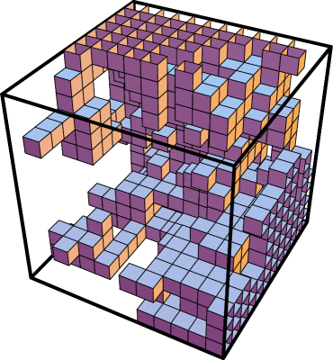
FIG. 1.: Example of excitation found for a $12^{3}$ lattice with free boundary conditions.

Such a cluster has a very non-trivial topology and is thus very far from being domain-wall like. This motivates the following three-fold classification of the events we obtain when considering free boundary conditions. In the first class, a cluster and its complement touch all $6$ faces of the cube. In the second class, a cluster touches at most $3$ faces of the cube. The third class consists of all other events. Finite size droplets should asymptotically always fall into the second class, albeit with finite size corrections of order $L^{-\theta_{l}}$.

Does the first class constitute a non-zero fraction of all events? At finite $L$, we find the following fractions: $23.3\%$ $(L=5)$, $23.9\%$ $(L=6)$, $25.1\%$ $(L=7)$, $24.4\%$ $(L=8)$, $25.0\%$ $(L=9)$, $25.7\%$ $(L=10)$, and $26.0\%$ $(L=11)$. The trend of these numbers suggests that the first class does indeed encompass a finite fraction of all the events when $L\to\infty$. We also considered the scaling of cluster sizes with $L$. Fig. 2 shows $Q(v,1/2)$ as a function of $v=V/L^{3}$, restricted to events belonging to the first class. (The $v=0$ values are the fractions we just gave above.) The curves for different $L$ show a small drift, $Q(v,1/2)$ growing with $L$. We consider this drift to be a finite size effect and that the correct interpretation of our data is $\theta_{g}\approx 0$, in agreement with the mean field picture. Our conclusion is then that as $L\to\infty$, there is a finite probability of having an $O(1)$ energy excitation that is non-domain-wall like, the cluster and its complement touching all faces of the cube.

FIG. 2.: Integrated probability $Q(v,1/2)$ of events in the first class. (From bottom to top, $L=5,7,9,11$.

Surface to volume ratios —

Obviously the mean field picture obtained by extrapolating results from the SK or Viana-Bray spin glasses cannot teach us anything about the topology of excitations for three-dimensional lattices. But mean field may serve as a guide for other properties such as the link overlap $q_{l}$ between ground states and excited states. In the SK model, the spin overlap $q\equiv\sum S_{i}S_{i}^{\prime}/N$ and the link overlap $q_{l}\equiv\sum(S_{i}S_{j})(S_{i}^{\prime}S_{j}^{\prime})/(N(N-1)/2)$ satisfy $q_{l}=q^{2}$, and both $q$ and $q_{l}$ have non-trivial distributions. Extrapolating this to our three dimensional system, the mean field picture predicts that the clusters associated with large scale excitations both span the whole system (as we saw with free boundary conditions) and are space filling. Quantitatively, this implies that their surface grows as the total volume of the system, i.e., as $L^{3}$.

To investigate this question, we have measured the surface of our excitations, defined as the number $S$ of links connecting the corresponding cluster to its complement. (Then $q_{l}=1-2S/3L^{3}$.) In figure 3 we show the mean value of $S/L^{3}$ as a function of $L$ for $v=V/L^{3}$ belonging to the three intervals $]0.20,0.25]$, $]0.30,0.35]$, and $]0.40,0.45]$. The data shown are for free boundary conditions, but the results are very similar for periodic boundary conditions. The most striking feature is that the curves decrease very clearly with $L$. For each interval, we have fitted the data to $\langle S\rangle/L^{3}=A+B/L^{\mu}$ and to a polynomial in $1/L$. Of major interest is the value of the constant because it gives the large $L$ limit of the curves.

Table I summarizes the quality of the fits as given by their $\chi^{2}_{r}$ (chi squared per degree of freedom). In all cases the fits are reasonably good; this is not so surprizing because our range of $L$ values is small. The most reliable fits are obtained using a quadratic polynomial in $1/L$, this functional form leading to a smooth and monotone behavior of the parameters and to small uncertainties in the parameters. For the large $L$ limits, these fits give $A=0.22$, $A=0.27$ and $A=0.30$ for the three intervals. (We do not give results for the linear fits which on the contrary are very poor.) The constant plus power fits also have good $\chi^{2}_{r}$ but the $A$s obtained were small and decreased with $v$; also they had large uncertainties and seemed to be compatible with $A=0$. Because of this, we also performed fits of the form $\langle S\rangle/L^{3}=B/L^{\mu}$. These are displayed in Fig. 3 and lead to $\mu\approx 0.30$ (the exponent varies little from curve to curve), again with reasonable $\chi^{2}_{r}$s. Because of this, we feel we cannot conclude from the data that the surface to volume ratios tend towards a non-zero asymptote. What can be said is that this asymptote seems to be small, and that it will be difficult to be sure that it is non-zero without going to larger values of $L$.

FIG. 3.: Mean value of surface to $L^{3}$ ratios for $v=V/L^{3}$ in intervals around $0.225,0.325,0.425$ (bottom to top) using free boundary conditions. Curves are pure power fits.

Interval	$A+B/L^{\mu}$	$A+B/L+C/L^{2}$	$B/L^{\mu}$
$]0.20,0.25]$	0.6	0.6	2.0
$]0.30,0.35]$	1.1	1.1	1.5
$]0.40,0.45]$	0.7	0.9	0.6

TABLE I.: Chi squared per degree of freedom for the fits to the data of Fig. 3.

Discussion —

For the three dimensional Edwards-Anderson spin glass model, we have presented numerical evidence that it is possible to flip a finite fraction of the whole lattice at an energy cost of $O(1)$, corresponding to $\theta_{g}\approx 0$ as predicted by mean field. This property transpired most clearly through the use of free boundary conditions, allowing one to conclude that $\theta_{g}\approx 0$ is not an artefact of trapped domain walls caused by periodic boundary conditions. Extrapolating to finite temperature, we expect the equilibrium $P(q)$ to be non trivial as in the mean field picture.

The other messages of our work concern the nature of these large scale excitations whose energies are $O(1)$. First, using free boundary conditions, we found them to be topologically highly non-trivial: with a finite probability they reach the boundaries on all 6 faces of the cube. Thus they are not domain-wall-like, rather they are sponge-like. Second, our data (both for periodic and free boundary conditions) indicate very clearly that their surface to volume ratios decrease as $L$ increases. The most important issue here is whether or not these ratios decrease to zero in the large $L$ limit. Although our data are compatible with a non-zero limiting value as predicted by mean field, the fits were not conclusive so further work is necessary.

If the surface to volume ratios turned out to go to zero, we would be lead to a new scenario that we have coined “TNT”. In the standard mean field picture, the surface to volume ratios cannot go to zero; indeed in the SK and Viana-Bray spin glass models there are no spin clusters with surface to volume ratios going to zero. However, in finite dimensions, one can have surface to volume ratios going to zero, in which case $q_{l}\to 1$. This property would then lead to a non-trivial $P(q)$ but to a trivial $P(q_{l})$. This trivial-non-trivial (TNT) scenario does not seem to have been proposed previously.

Perhaps the most dramatic consequence of this new scenario is for window overlaps in spin glasses: because in TNT one is asymptotically always in the bulk of an excitation, correlation functions at any finite distance will show no effects of replica symmetry breaking. That this may arise in fact is supported by work by Palassini and Young[7] who showed that certain window overlaps seemed to become trivial as $L\to\infty$. (See also [8] for a similar discussion in two-dimensions.) These authors referred to this property as evidence for a “trivial ground state structure”. But in our picture the global (infinite distance) structure is non-trivial, as indicated by $\theta_{g}=0$, in sharp contrast to the droplet/scaling picture. Also, in very recent work [9], Palassini and Young have extended their previous investigations and have extracted excited states by a quite different method from ours, and they find that their data is compatible with the TNT scenario. Naturally, there is also evidence in favor of the non-triviality of window overlaps [10]. Nevertheless, we believe that our mixed scenario is a worthy candidate to describe the physics of short range spin glasses. Furthermore, its plausibility should not restricted to $3$ dimensions, it could hold in all dimensions greater than $2$. (Note that in $d=2$, excitations are necessarily topologically trivial.) An important indication of this was obtained by Palassini and Young whose computations [9] favor the TNT scenario over the droplet picture in the 4-dimensional Edwards-Anderson model.

REFERENCES

- [1] Spin Glasses and Random Fields, edited by A. P. Young (World Scientific, Singapore, 1998).
- [2] M. Mézard, G. Parisi, and M. A. Virasoro, Spin-Glass Theory and Beyond, Vol. 9 of Lecture Notes in Physics (World Scientific, Singapore, 1987).
- [3] D. S. Fisher and D. A. Huse, Phys. Rev. B 38, 386 (1988).
- [4] A. J. Bray and M. A. Moore, in Heidelberg Colloquium on Glassy Dynamics, Vol. 275 of Lecture Notes in Physics, edited by J. L. van Hemmen and I. Morgenstern (Springer, Berlin, 1986), pp. 121–153.
- [5] J. Houdayer and O. C. Martin, Euro. Phys. Lett. 49, 794 (2000).
- [6] J. Houdayer and O. C. Martin, Phys. Rev. Lett. 83, 1030 (1999).
- [7] M. Palassini and A. P. Young, Phys. Rev. Lett. 83, 5126 (1999).
- [8] A. Middleton, Phys. Rev. Lett. 83, 1672 (1999).
- [9] M. Palassini and A. P. Young, private communication.
- [10] E. Marinari et al., J. Stat. Phys. 98, 973 (2000).