Lévy Distribution of Single Molecule Line Shape Cumulants in Low Temperature Glass

Abstract

Abstract

We investigate the distribution of single molecule line shape cumulants, $\kappa_{1},\kappa_{2},\cdots$, in low temperature glasses based on the sudden jump, standard tunneling model. We find that the cumulants are described by Lévy stable laws, thus generalized central limit theorem is applicable for this problem.

Pacs: 05.40.-a, 05.40.Fb, 61.43.FS, 78.66.Jg

Recent experimental advances [1] have made it possible to measure the spectral line shape of a single molecule (SM) embedded in a condensed phase. Because each molecule is in a unique static and dynamic environment, the line shapes of chemically identical SMs vary from molecule to molecule [2]. In this way, the dynamic properties of the host are encoded in the distribution of single molecule spectral line shapes [1, 2, 3, 4, 5, 6, 7, 8, 9]. We examine the statistical properties of the line shapes and show how these are related to the underlying microscopic dynamical events occurring in the condensed phase.

We use the Geva–Skinner [5] model for the SM line shape in a low temperature glass based on the sudden jump picture of Kubo and Anderson [10, 11]. In this model, a random distribution of low–density (and non–interacting) dynamical defects [e.g., spins or two level systems (TLS)] interacts with the molecule via long range interaction (e.g., dipolar). We show that Lévy statistics fully characterizes the properties of the SM spectral line both in the fast and slow modulation limits, while far from these limits Lévy statistics describes the mean and variance of the line shape. We then compare our analytical results, derived in the slow modulation limit, with results obtained from numerical simulation. The good agreement indicates that the slow modulation limit is correct for the parameter set relevant to experiment.

Lévy stable distributions serve as a natural generalization of the normal Gaussian distribution. The importance of the Gaussian in statistical physics stems from the central limit theorem. Lévy stable laws are used when analyzing sums of the type $\sum x_{i}$, with $\{x_{i}\}$ being independent identically distributed random variables characterized by a diverging variance. In this case the ordinary Gaussian central limit theorem must be replaced with the generalized central limit theorem. With this generalization, Lévy stable probability densities, $L_{\gamma,\eta}(x)$, replace the Gaussian of the standard central limit theorem. Khintchine and Lévy found that stable characteristic functions, $\hat{L}_{\gamma,\eta}(k)$, are of the form [12]

$$\ln\left[\hat{L}_{\gamma,\eta}\left(k\right)\right]=i\mu k-z_{\gamma}|k|^{\gamma}\left[1-i\eta{k\over|k|}\tan\left({\pi\gamma\over 2}\right)\right]$$ (1)

for $0<\gamma\leq 2$ (for the case $\eta\neq 0$, $\gamma=1$ see [12]). Four parameters are needed for a full description of a stable law. The constant $\gamma$ is called the characteristic exponent, the parameter $\mu$ is a location parameter which is unimportant in the present case, $z_{\gamma}>0$ is a scale parameter and $-1\leq\eta\leq 1$ is the index of symmetry. When $\eta=0$ $(\eta=\pm 1)$ the stable density $L_{\gamma,\eta}(x)$ is symmetrical (one sided). Lévy statistics is known to describe several long range interaction systems in diverse fields such as astronomy [12], turbulence [13] and spin glass [14]. Stoneham’s theory [15] of inhomogeneous line broadening in defected crystal, is based on long-range forces and parts of it can be interpreted in terms of Lévy stable laws [9]. Stoneham’s approach [15] is inherently static, while the SM line shape model considers both dynamical and static contributions from the defects.

An important issue is the slow and fast modulation limits [6, 11]. Briefly, the fast (slow) modulation limit is valid if important contributions to the line shape are from TLSs which satisfy $\nu\ll K$ $(\nu\gg K)$, where $\nu$ is the frequency shift of the SM due to SM–TLS interaction and $K$ is the transition rate of the flipping TLS (see details below). In the fast modulation limit, all (or most) lines are Lorentzian with a width that varies from one molecule to the other. For this case, the (Lévy) distribution of line widths fully characterizes the statistical properties of the lines. The second, more complicated, case corresponds to the slow modulation limit. Then the SM line is typically composed of several peaks (splitting) and is not described well by a Lorentzian. If a SM shows splitting, one can investigate the validity of the standard tunneling model of glass [16] in a direct way, since the splitting of a line is directly associated with SM–TLS interaction [7]. As mentioned, we demonstrate the existence of a slow modulation limit in SM–glass system.

Following [5] we assume a SM coupled to non identical independent TLSs at distances ${\bf r}$ in dimension $d$. Each TLS is characterized by its asymmetry variable $A$ and tunneling element $J$. The energy of the TLS is $E=\sqrt{A^{2}+J^{2}}$. The TLSs are coupled to phonons or other thermal excitations such that the state of the TLS changes with time. The state of the $n$ th TLS is described by an occupation parameter, $\xi_{n}(t)$, that is equal $0$ or $1$ if the TLS is in its ground or excited state respectively. The probability for finding the TLS in its upper $\xi=1$ state, $p$, is given by the standard Boltzmann form $p=1/\{1+\exp[E/(k_{b}T)]\}$. The transitions between the ground and excited state are described by the up and down transition rates $K_{u},K_{d}$, which are related to each other by the standard detailed balance condition.

The excitation of the $n$ th TLS shifts the SM’s transition frequency by $\nu_{n}$. Thus, the SM’s transition frequency is

$$\omega(t)=\omega_{0}+\sum_{n=1}^{N_{\rm act}}\xi_{n}\left(t\right)\nu_{n},$$ (2)

where $N_{\rm act}$ is the number of active TLSs in the system (see details below) and $\omega_{0}$ is the bare transition frequency that differs from one molecule to the other depending on the local static disorder. We consider a wide class of frequency perturbations

$$\nu=2\pi\alpha\Psi\left(\Omega\right)f\left(A,J\right){1\over r^{\delta}},$$ (3)

$\alpha$ is a coupling constant with units $\left[\mbox{Hz}\ \mbox{nm}^{\delta}\right]$, $\Psi\left(\Omega\right)$ is a dimensionless function of order unity, $\Omega$ is a vector of angles determined by the orientations of the TLS and molecule (in some simple cases $\Omega$ depends on polar angles only), $f(A,J)\geq 0$ is a dimensionless function of the internal degrees of freedom of the fluctuating TLS, $\delta$ is the interaction exponent. The line shape of the SM is given by the complex Laplace transform of the relaxation function

$$I_{SM}\left(\omega\right)={1\over\pi}\mbox{Re}\left[\int_{0}^{\infty}dte^{i\omega t}\Pi_{n=1}^{N_{\rm act}}\Phi_{n}\left(t\right)\right]$$ (4)

provided that the natural life time of the SM excited state is long. The relaxation function of a single TLS was evaluated [11] based on methods developed in [10]

$$\Phi\left(t\right)=e^{-\left(\Xi+ip\nu\right)t}\left[\cosh\left(\Omega t\right)+{\Xi\over\Omega}\sinh\left(\Omega t\right)\right]$$ (5)

with $\Omega=[K^{2}/4-\nu^{2}/4-i\left(p-1/2\right)\nu K]^{1/2}$, $\Xi={K\over 2}-i\left(p-{1\over 2}\right)\nu$ and $K=K_{u}+K_{d}$. For a bath of TLSs the line shape, Eq. (4), is a formidable function of the random TLS parameters $(r,\Omega,A,J)$ as well as the system parameters $(\alpha,T,\mbox{etc})$. In the fast modulation limit $K\gg|\nu|$, one finds a simpler behavior: all lines are Lorentzian with half width

$$\tilde{\Gamma}=\sum_{n}^{N_{act}}p_{n}(1-p_{n})\nu_{n}^{2}/K_{n}$$ (6)

which varies from one molecule to the other. Eq. (6) shows the well known phenomena of motional narrowing. In the slow modulation limit $K\ll|\nu|$ one finds $\Phi(t)=1-p+pe^{-i\nu t}$ implying that the line shape of a molecule coupled to a single TLS is composed of two delta peaks, the line shape of a molecule coupled to two TLSs is composed of four delta peaks, etc (splitting).

The spectral line is characterized by its cumulants $\kappa_{j}$ $(j=1,2,\cdots)$ that vary from one molecule to the other, and we investigate the cumulant probability density $P(\kappa_{j})$. We have derived the cumulants of the SM line shape, and the first four cumulants are presented in Table 1 [17]. We observe that cumulants of order $j\leq 2$ are real while generally cumulants of order $j>2$ are complex, implying that the moments of the line shape diverge when $j>2$. The summation, $\sum_{n}$, in Table $1$ is over the active TLSs, namely those TLSs which flip on the time scale of observation $\tau$ (i.e., $K_{n}>1/\tau$). We consider the slow modulation limit, soon to be justified, which means that we consider the case $K_{n}\ll\nu_{n}$. To investigate this limit we set $K_{n}=0$ in Table $1$, then all the cumulants are real and are rewritten as $\kappa_{j}=\sum_{n}H_{jn}\nu_{n}^{j}$, where $H_{j}$ are functions of $p$ only and $H_{1}=p$, $H_{2}=p(1-p)$, $H_{3}=p(1-p)(2p-1)$ etc. Note that for $\kappa_{1}$ and $\kappa_{2}$ no approximation is made.

j	$\kappa_{j}$
$1$	$\sum_{n}p_{n}\nu_{n}$
$2$	$\sum_{n}p_{n}\left(1-p_{n}\right)\nu_{n}^{2}$
$3$	$\sum_{n}p_{n}\left(1-p_{n}\right)\left(2p_{n}-1\right)\nu_{n}^{3}+i\sum_{n}p_{n}(1-p_{n})K_{n}\nu_{n}^{2}$
$4$	$\sum_{n}p_{n}\left(-1+p_{n}\right)\left[K_{n}^{2}+\nu_{n}^{2}\left(-1+6p_{n}-6p_{n}^{2}\right)\right]\nu_{n}^{2}-$
	$2i\sum_{n}K_{n}\left(-1+p_{n}\right)p_{n}\left(-1+2p_{n}\right)\nu_{n}^{3}$

Table 1: Cumulants $$\kappa_{j}$$ of the SM line shape

Let $\left\langle\cdot\right\rangle_{r\Omega AJ}$ denote an averaging over the random TLS parameters. The characteristic function of the $j$ cumulant can be written in a form

$$\left\langle\exp\left(ik\kappa_{j}\right)\right\rangle_{r\Omega AJ}=$$

$$\exp\left[-\rho_{\mbox{eff}}\left\langle\int d\Omega\int_{0}^{\infty}{d(r^{d})\over d}\left(1-e^{ikB_{j}/r^{\delta j}}\right)\right\rangle_{AJ}\right],$$ (7)

$\rho_{\mbox{eff}}$ is the density of the active TLS and $B_{j}=(2\pi\alpha)^{j}\Psi^{j}\left(\Omega\right)f^{j}\left(A,J\right)H_{j}$. To derive Eq. (7) we have used the assumption of independent TLSs uniformly distributed in the system. For odd $j$ cumulants we find

$$\left\langle\exp\left(ik\kappa_{j}\right)\right\rangle_{r\Omega AJ}=\hat{L}_{\gamma,0}(k),$$ (8)

with characteristic exponent $\gamma=d/(\delta j)$ and the scale parameter

$$z_{\gamma}=\rho_{\mbox{eff}}\left(2\pi\alpha\right)^{{d\over\delta}}\left\langle f^{d/\delta}\left(A,J\right)|H_{j}|^{\gamma}\right\rangle_{AJ}c_{\gamma}\int d\Omega|\Psi^{j}\left(\Omega\right)|^{\gamma}$$ (9)

with $c_{\gamma}=\cos\left(\gamma\pi/2\right)\Gamma(1-\gamma)$, $c_{1}=\pi/2$. Eq. (8) shows that odd cumulants are described by symmetrical Lévy stable density, i.e., $P(\kappa_{j})=L_{\gamma,0}(\kappa_{j})$. Two conditions must be satisfied for such a behavior, $0<\gamma<2$ and $\int d\Omega\sin\left[\Psi^{j}(\Omega)\right]=0$. The latter condition gives the symmetry condition, $\eta=0$, which means that negative and positive contributions to $\kappa_{j}$ are equally probable.

For even cumulants and $0<\gamma<1$ we find

$$\left\langle\exp\left(ik\kappa_{j}\right)\right\rangle_{r\Omega AJ}=\hat{L}_{\gamma,\eta}(k)$$ (10)

with a scale parameter Eq. (9) and with Lévy index of symmetry

$$\eta={\left\langle f^{j\gamma}\left(A,J\right)|H_{j}|^{\gamma}{H_{j}\over|H_{j}|}\right\rangle_{AJ}\over\left\langle f^{j\gamma}\left(A,J\right)|H_{j}|^{\gamma}\right\rangle_{AJ}}.$$ (11)

Eq. (10) implies that even cumulants are distributed according to $P(\kappa_{j})=L_{\gamma,\eta}(\kappa_{j})$. We note that the asymmetrical Lévy functions, with $\eta\neq\pm 1,0$, only rarely find their applications in the literature. The characteristic exponent $\gamma$ depends only on the general features of the model (namely on $d$ and $\delta$). In contrast the Lévy index of symmetry $\eta$ depends on the details of the model and on system parameters $(T,\mbox{etc})$. For $j=2$ we have $H_{j}=|H_{j}|$ and then $\eta=1$ so the Lévy density is one sided, as is expected since $\kappa_{2}>0$.

As mentioned, in the fast modulation limit, the random line width in Eq. (6) characterizes the statistical properties of the spectral lines. Using the approach in Eqs. (7-9) one can show that $P(\tilde{\Gamma})=L_{d/(2\delta),1}(\tilde{\Gamma})$ with the scale parameter $z_{d/(2\delta)}$ given by Eq. (9) with $j=2$ and $H_{2}=p(1-p)/K$.

In what follows we exhibit our results and compare to simulations based on the standard tunneling model of low temperature glass [16]. We use system parameters given by Geva and Skinner [5] to model terrylene in polystryrene. The SM-TLS interaction is dipolar, hence $\delta=3$, and we consider spatial dimension $d=3$. The distribution of the asymmetry parameter and tunneling element is $P(A)P(J)=N^{-1}J^{-1}$ for $2.8\times 10^{-7}{\rm K}<J<18{\rm K}$ and $0<A<17{\rm K}$, $N$ denoting a normalization constant. We use $f(A,J)=A/E$ and define a TLS to be active if $K>1/\tau$, $\tau=120$ sec is the time of experimental observation. In this way the averaging $\left\langle\cdots\right\rangle_{AJ}$ becomes $\tau$ independent. The rate of the TLS is given by $K=cJ^{2}E\coth\left({\beta E_{n}/2}\right)$ and $c=3.9\times 10^{8}{\rm K}^{-3}$Hz is the TLS phonon coupling constant. Additional system parameters are the coupling constant $\alpha=3.75\times 10^{11}$ $\mbox{nm}^{3}$Hz and the TLS density $1.15\times 10^{-2}$ nm^-3. According to Eqs. (8)-(11), only the scale parameter $z_{\gamma}$ depends on the orientation of the TLS and SM, through $\Psi(\Omega)$. It is therefore reasonable to assume simple forms for $\Psi(\Omega)$. We consider two examples, model $1$ ($\mbox{M}1$) for which $\Psi(\Omega)$ is replaced with a two state variable (i.e., a spin model) $\Psi=1$ or $\Psi=-1$ with equal probabilities of occurrence and model $2$ ($\mbox{M}2$) $\Psi(\Omega)=\cos(\theta)$, with $\theta$, the standard polar coordinate, distributed uniformly. With these definitions we calculate the symmetry index $\eta$ and the scaling parameter $z_{\gamma}$ and compare between the theory and numerical simulation.

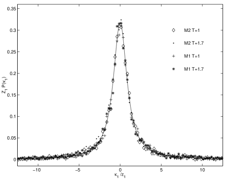
FIG. 1.: Scaled probability density of first cumulant $P(\kappa_{1})z_{1}$ versus $\kappa_{1}/z_{1}$. Symbols are the simulation results obtained from $4000$ molecules for different cases indicated in the figure. The theory, plotted as a solid curve, predicts a Lorentzian density $P(\kappa_{1})=L_{1,0}(\kappa_{1})$ with a scaling parameter $z_{1}$ which varies from one set of data to the other.

We consider the first two cumulants $\kappa_{1}$ and $\kappa_{2}$ (i.e, the line shape mean and variance). Since $d=\delta$ we find $P(\kappa_{1})=L_{1,0}(\kappa_{1})$ which is the Lorentzian density, and $P(\kappa_{2})=L_{1/2,1}(\kappa_{2})$ which is Smirnov’s density. We have considered two temperatures for the two models M1 and M2. As shown in Fig. 1 and 2, a scaling behavior is observed and all data collapse on the Lévy densities $L_{1,0}(\kappa_{1})$ and $L_{1/2,1}(\kappa_{2})$ respectively. In Fig. 1 and 2 we have rejected TLSs within a sphere of radius $r_{\rm min}=1$ nm, demonstrating that our results are not sensitive to a short cutoff. Also shown in the inset of Fig. 2 is $P(\mbox{Re}[\kappa_{3}])$ which is distributed according to $L_{1/3,0}(\mbox{Re}[\kappa_{3}])$ and a scale parameter $z_{1/3}$ given in Eq. (9). The Lévy behavior of $\kappa_{1},\kappa_{2}$ and $\mbox{Re}[\kappa_{3}]$ holds generally and is not limited to the slow modulation limit since these random variables do not depend explicitly on the rates $K$.

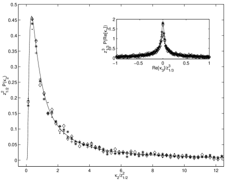
FIG. 2.: Same as Fig. (1) for the second cumulant. We show $P(\kappa_{2})z_{1/2}^{2}$ versus $\kappa_{2}/z_{1/2}^{2}$. The solid curve is Smirnov’s density $L_{1/2,1}(\kappa_{2})$. In the inset we show the same as Fig. (1) for $\mbox{Re}[\kappa_{3}]]$, the solid curve is Lévy density $L_{1/3,0}(\mbox{Re}[\kappa_{1/3}])$.

Consider the distribution of $\mbox{Re}[\kappa_{4}]$, which in the slow modulation limit is distributed according to $L_{1/4,\eta}(\mbox{Re}[\kappa_{4}])$, Eq. (10). The question remains if such a slow modulation limit is valid for the standard tunneling model parameters we are considering. The slow modulation limit is expected to work when $K\ll|\nu|$. For large enough $r$ this inequality will fail; however, depending on system parameters, we expect that contributions from TLS situated far from the SM are negligible. We also note that according to the standard tunneling model the rates $K$ are distributed over a broad range, albeit with finite cutoffs that insure that the averaged rate is finite. To check if the slow modulation limit is compatible with the standard tunneling model approach, we compare our slow modulation results with those obtained by simulation in Fig. 3. We also show simulation results in which all rates are set to zero ($K=0$). For model $\mbox{M}1$, we find that the deviation between simulation and theory is small so the assumption of slow modulation limit is justified. For model $\mbox{M}2$, we see slightly larger deviations between the theory and numerical results, due to the angular dependence of model $\mbox{M}2$, $\Psi(\Omega)=\cos(\theta)$, which reduces the typical frequency shift $|\nu|$ compared to model $\mbox{M}1$. We conclude that the present theory can be used as a criterion for the validity of the slow modulation limit.

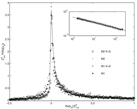
FIG. 3.: Same as Fig. (1) for $Re[\kappa_{4}]$ and for temperature $T=1.7{\rm K}$. The symbols are the simulation results obtained for four different cases as indicated in the figure and for $12000$ molecules. The solid curve is $L_{1/4,\eta}[\mbox{Re}(\kappa_{4})]$ with an index of asymmetry $\eta=0.6104$. In the inset we show the power law tail of the scaled probability density on a log-log plot.

Depending on system parameters, Lévy statistics may become sensitive to the finite cutoff $r_{\rm min}$, Physically, the cutoff can be important since the power low interaction is not supposed to work well for short distances [6]. Our results were derived for $r_{\rm min}=0$, while for small though finite $r_{\rm min}$ one can find intermittency behavior, i.e., the ratio $\langle\kappa_{2}^{2}\rangle/\langle\kappa_{2}\rangle^{2}$ (as well as similar dimensionless ratios) is very large. When $r_{\rm min}$ is large one finds a Gaussian behavior. The phenomena of intermittency in the context of a reaction of a SM in a random environment was investigated in [18]. Generally high order cumulants are more sensitive to finite cutoff and for results in Fig (3) $r_{\rm min}=0$ was chosen to see the proper decay laws in the wing.

To conclude, we showed that the generalized central limit theorem can be used to analyze distribution of cumulants of SM line shapes in glass. We note that besides cumulants, Lévy statistics can be used to analyze other statistical properties of SMs in disordered media [9].

Acknowledgment EB thanks the ETH and Prof. Wild for their hospitality. This work was supported by the NSF.

REFERENCES

- [1] W. E. Moerner and M. Orrit, Science 283 5408 (1999). T. Plakhotnik, E. Donley and U. P. Wild, Annu. Rev. Phys. Chem. 48, 181 (1997) and references therein.
- [2] L. Fleury, A. Zumbusch, M. Orrit, R. Brown and J. Bernard, J. Lumin. 56 15 (1993). J. Tittel, R. Kettner, Th. Basche, C. Brauchle, H. Quante, K. Mullen, J. Lumin. 64 1 (1995). M. Vacha, Y. Liv, H. Nakatsuka, T. Tani, J. Chem. Phys. 106 8324 (1997). B. Kozankiewicz, J. Bernard and M. Orrit, J. Chem. Phys, 101 9377 (1994).
- [3] P. D. Reilly and J. L. Skinner, Phys. Rev. Lett. 71 4257 (1993).
- [4] G. Zumofen and J. Klafter, Chem. Phys. Lett. 219 303 (1994).
- [5] E. Geva and J. L. Skinner, J. Phys. Chem. B 101 8920 (1997). E. Geva and J. L. Skinner, Chem. Phys. Lett. 287 125 (1998).
- [6] W. Pfluegl, F. L. H. Brown and R. J. Silbey, J. Chem. Phys. 108 6876 (1998).
- [7] A. M. Boiron, P. Tamarat, B. Lounis, R. Brown and M. Orrit, J. Chem. Phys. 247 119 (1999).
- [8] E. Barkai and R. Silbey, Chem. Phys. Lett., 310 287 (1999).
- [9] E. Barkai and R. Silbey, (submitted).
- [10] P. W. Anderson, J. Phys. Soc. Jpn. 9, 316 (1954). R. Kubo, ibid 6 935 (1954).
- [11] P. D. Reilly and J. L. Skinner, J. Chem. Phys. 101 (2) 959 (1994).
- [12] W. Feller,An introduction to probability Theory and Its Applications Vol. 2 (John Wiley and Sons 1970).
- [13] S. G. Llewellyn Smith and S. T. Gille Phys. Rev. Lett. 81 5249 (1998) and references therein.
- [14] Y. Furukawa, Y. Nakai and N. Kunitomi, J. of the Phys. Soc. Japan 62 No.1. 306 (1993).
- [15] A. M. Stoneham, Rev. Mod. Phys. 41 82 (1969).
- [16] P. W. Anderson, B. I. Halperin, C. M. Varma, Philos. Mag. 25, 1 (1971). W. A. Philips, J. Low. Temp. Phys. 7, 351 (1972).
- [17] In Table 1 we use , for we have while the higher order cumulants are independent. The distribution of depends on the static disorder [15] while we are considering the dynamic disorder due to the flipping TLSs.
- [18] J. Wang and P. Wolynes, Phys. Rev. Lett. 74 4317 (1995).