0pt0.4pt 0pt0.4pt 0pt0.4pt

Probing Pseudogap by Josephson Tunneling

Abstract

We propose here an experiment aimed to determine whether there are superconducting pairing fluctuations in the pseudogap regime of the high-$T_{c}$ materials. In the experimental setup, two samples above $T_{c}$ are brought into contact at a single point and the differential AC conductivity in the presence of a constant applied bias voltage between the samples, $V$, should be measured. We argue the the pairing fluctuations will produce randomly fluctuating Josephson current with zero mean, however the current-current correlator will have a characteristic frequency given by Josephson frequency $\omega_{J}=2eV/\hbar$. We predict that the differential AC conductivity should have a peak at the Josephson frequency with the width determined by the phase fluctuations time.

One of the long-standing puzzles of the high-temperature superconductivity is the nature of the so-called pseudogap regime. The pseudogap regime occurs in the wide range of temperatures above superconducting transition temperature in the underdoped cuprate superconductors. It is characterized by the suppressed quasiparticle density of states in the vicinity of the Fermi level. The similarity of the density of states in the pseudogap regime and in the superconducting state lead many [1] to believe that that the pseudogap itself is of a superconducting origin. In this view, the long range superconducting order in the pseudogap regime is destroyed by phase fluctuations. However, locally, both electronic pairing and fluctuating regions of superconductivity should persist. Therefore, in this picture, the superconducting phase transition is believed to be a superconducting phase-ordering transition. Moreover, recent experiments by Orenstein and collaborators claim that local superfluid density is present even above $T_{c}$ in Bi2212 materials [2].

Whether or not the pseudogap indeed has a superconducting origin remains to be verified experimentally. Such standard experimental test as the vanishing resistivity, or the Meissner effect are bound to fail. Both these test require spatial and temporal stability of the superconducting phase on the time scale of the experiment. On the other hand, the pseudogap state can at best have superconducting order parameter that varies both in space and in time. A successful test may be possible if the fluctuations could somehow be stabilized by the proximity to a “real” superconductor [3]. Another approach is to probe superconductivity locally in space on the time scales comparable or shorter than the characteristic time of the phase fluctuations.

In this letter we propose the first experiment of this type, which is based on the AC Josephson effect. The main point we make is that in the presence of phase fluctuations Josephson current $j(t)$ across the tunneling contact is a random time-dependent quantity. It has a dispersion that is the current-current correlator $\langle j(t)j(t^{\prime})\rangle$, which is related to the corrections to the conductivity across the junction. This current-current correlator “remembers” about its Josephson origin and has a scale set by Josephson frequency and phase fluctuation time. Therefore, the conductivity of a junction will have a correction due to current fluctuations,

$$\Delta\sigma\propto 1/V,$$ (1)

where $V$ is the applied voltage across the junction. The crucial new aspect of the proposed approach is that we will focus on the characteristic time scale of frequency fluctuations, assuming that tunneling occurs in a small region where the spatial dependence can be ignored. We will focus on the time dynamics of the phase fluctuations in our analysis.

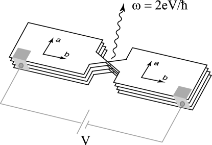
FIG. 1.: Consider two parts of a superconductor brought into a tunneling contact at a temperature $T>T_{c}$, so that the phase of the order parameter is no longer stationary. Our approach is to consider the Josephson current (Eq. 2) as a randomly fluctuating quantity, with the three major sources of randomness: the amplitude noise, the frequency noise, and the phase noise. We also assume that the contact is small enough for the superconducting parameters to be spatially uniform in the vicinity of the contact.

When two pieces of a superconductor are joined by a weak link, a superconducting current begins to flow through the link in the absence of applied voltage between the superconductors. The current is related to the difference of the phases $\phi_{1}$ and $\phi_{2}$ of the superconductors,

$$j=j_{0}\sin(\phi_{1}-\phi_{2}),$$ (2)

with the parameter $j_{0}$ related to the coupling strength between the two superconductors. For a superconductor in an equilibrium, evolution of the phase,

$${\partial\phi}/{\partial t}=-2\mu/\hbar,$$ (3)

is determined[5] by the superconductor chemical potential, $\mu$. Therefore, the phase as a function of time is $\phi(t)=-2\mu t/\hbar+\phi_{0}$, where $\phi_{0}$ is the phase at time $t=0$. For two coupled superconductors the phase difference evolves as

$$\phi_{1}(t)-\phi_{2}(t)=2(\mu_{2}-\mu_{1})t/\hbar+\phi_{1}(0)-\phi_{2}(0).$$ (4)

The difference of the chemical potentials equals the applied voltage, $\mu_{2}-\mu_{1}=eV$. Hence, if $V=0$, both the phase difference and the current given by Eq. (2) remain constant. However, in the presence of a bias, $V$, the phase difference grows linearly with time and the current oscillates according to

$$j(t)=j_{0}(\omega_{J})\sin(\omega_{J}t+\Delta\phi),$$ (5)

with the frequency $\omega_{J}=2eV/\hbar$ and the initial phase $\Delta\phi=\phi_{1}(0)-\phi_{2}(0)$. The effect of generating an alternating current by applying a constant bias to a superconducting tunnel junction is called AC Josephson effect. An important feature of this effect is that the frequency of the generated current is only a function of the applied bias voltage and is independent of the microscopic and macroscopic parameters of the system. The scale of the frequency is about 0.5 $\Gamma$Hz per 1 microvolt. The AC Josephson effect is routinely observed in the superconducting regime. It can be observed either directly as the micro-wave emission from the oscillating current, or indirectly as “Shapiro steps” [6] in the DC $I-V$ curves measured in the presence of the oscillating bias voltage component.

For AC Josephson effect to be observable in the pseudogap regime, the measurement has to be local both in space and time. Suppose that above the transition temperature, superconductor can be modeled as a collection of superconducting islands of a characteristic size $L$, inside which phase fluctuates at a rate $\Lambda$. Then, if the size of a contact between two superconductors is less than $L$ then the superconducting state is essentially uniform in the vicinity of the contact. If the applied bias voltage is such that the Josephson frequency is larger than $\Lambda$ then the Josephson oscillations are faster than the phase fluctuations dynamics, and hence can be approximately modeled as

$$j(t)=j^{*}(\omega_{J},\Lambda,L)\sin(\omega_{J}t+\Delta\phi(t)),$$ (6)

with the amplitude $j^{*}$ being renormalized by spatial and temporal fluctuations of the superconducting phase. In general, the Josephson frequency can also fluctuate around its average value due to voltage fluctuations which are particularly important for small samples. However, we assume that these effects can be absorbed into the overall fluctuations of the phase, $\Delta\phi(t)$. It is important to note that both $\Lambda$ and $L$ are functions of temperature, with L and $1/\Lambda$ diverging at the superconducting transition. The parameter $L$ is related to the phase gradient correlation function $W$ considered by Franz and Millis [7]. Relationship between $\Lambda$ and $L$ is a subject of an active interest. In the vortex diffusion picture, where phase fluctuations are produced by moving vortices, $L$ is a distance vortex travels during the time $1/\Lambda$, namely $L=\sqrt{D/\Lambda}$. Here $D$ is the vortex diffusion constant. This corresponding dynamical critical exponent is $z=2$. Alternatively, if the phase fluctuations are governed by fast ballistic dynamics, the relation between the parameters $L$ and $\Lambda$ should be $L\Lambda=v^{*}$, where $v^{*}$ is propagation speed for the ballistic modes. This corresponds to $z=1$. Using different geometries in the experimental setup that we propose below may help to determine the relevant model.

A possible experimental setup that can be used to perform the measurement of the AC Josephson effect in the pseudogap regime is shown in the figure 1. The crucial aspect is that the point of contact between the superconductors be as small as possible. If the size of the contact becomes larger than $L$ then in addition to the temporal phase fluctuations a the point of contact one needs to include spatial fluctuations, which can lead to a significant suppression of the effect. Another desirable feature is that the two superconductors be only a few $ab$-planes thick. This is because the size of the superconducting “islands” is likely to be more extended in the planes, compared to across the planes. Hence, we believe that the effect we propose is more likely to be observed in the geometry of figure 1, although c-axis tunneling may also yield similar results. Finally, using very thin samples reduces the transition temperature [8], thereby making the pseudogap regime accessible at lower temperatures, where the thermal fluctuations are reduced.

There are several ways the oscillating super-current in the pseudogap regime can be detected. Here we consider two methods: 1) differential AC conductivity measurements in the presence of constant bias voltage, 2) detection of electro-magnetic radiation generated by the oscillating Josephson current. Although there is no coherent Josephson current in the pseudogap regime, the junction is expected to have strong response to the perturbations acting at the frequencies near $\omega_{J}$. Such super-current is also expected to generate a radiation peak at the frequency $\omega_{J}$, with a width of the peak governed by the phase fluctuations.

To make our qualitative arguments more formal we have to assign a particular form to the phase fluctuations. Here we make an assumption that the the phase difference between the superconductors, $\Delta\phi(t)$ follows a diffusion process, as shown in Fig. 2, with a variance

$$\langle(\Delta\phi_{t}-\Delta\phi_{t^{\prime}})^{2}\rangle=2\Lambda|t-t^{\prime}|.$$ (7)

and the initial phase $\Delta\phi_{0}$ distributed uniformly in the interval $[0,2\pi]$. The factor of 2 appears because for a weak tunnel junction the phases of on the both sides of the junction fluctuate independently, each at a rate $\Lambda$.

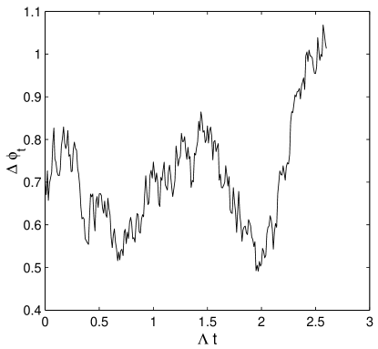
FIG. 2.: We assume here that the phase difference, $\Delta\phi_{t}$, between the superconductors forming the Josephson junction follows a one-dimensional geometrical Brownian walk as a function of time, $t$. Such process is defined by a linearly increasing with time dispersion, Eq. (7). The initial phase, $\Delta\phi_{0}$, is also a random quantity evenly distributed in the interval $[0,2\pi]$.

Viewing the Josephson current of Eq. (6) as a random quantity with a zero mean, we can characterize it by its dispersion and autocorrelation. The autocorrelation, according to the Kubo formula, determines the correction to the conductivity due to the fluctuating Josephson tunneling,

$$\Delta\sigma(\omega)=\frac{1}{\omega\nu}\int^{t}_{-\infty}{e^{i\omega(t-{t^{\prime}})}\langle j(t)j(t^{\prime})\rangle d{t^{\prime}}},$$ (8)

where brackets correspond to the $\phi$-averaging, and averaging over time $t$ is implied. Volume $\nu$ is necessary for normalization. Substituting expression for the current from Eq. (6), we obtain

$$\Delta\sigma = \frac{j^{*2}}{2\omega\nu}\int^{t}_{-\infty}{e^{i\omega(t-{t^{\prime}})}\langle\cos(\omega_{J}(t-{t^{\prime}})+\Delta\phi_{t}-\Delta\phi_{t^{\prime}})-}$$ (10)

$$\cos(\omega_{J}(t+{t^{\prime}})+\Delta\phi_{t}+\Delta\phi_{t^{\prime}})\rangle d{t^{\prime}}.$$

Since $\Delta\phi_{t}+\Delta\phi_{t^{\prime}}=(\Delta\phi_{t}-\Delta\phi_{0})+(\Delta\phi_{t^{\prime}}-\Delta\phi_{0})+2\Delta\phi_{0}$, after averaging over $\Delta\phi_{0}$ in the interval $[0,2\pi]$, the second cosine disappears. To average over $(\Delta\phi_{t}-\Delta\phi_{t^{\prime}})$, we invoke the relation $\langle\exp(iu)\rangle=\exp(-\langle u^{2}\rangle/2)$, valid for any normally distributed variable $u$ with a mean zero. Then after the integration we obtain

$$\Delta\sigma=\frac{j^{*2}}{4\omega\nu}\left[\frac{1}{\Lambda+i\omega-i\omega_{J}}+\frac{1}{\Lambda+i\omega+i\omega_{J}}\right].$$ (11)

As expected, the the real part of the conductivity,

$${\rm Re}(\Delta\sigma)=\frac{j^{*2}\Lambda}{4\omega\nu}\left[\frac{1}{(\omega-\omega_{J})^{2}+\Lambda^{2}}+\frac{1}{(\omega+\omega_{J})^{2}+\Lambda^{2}}\right],$$ (12)

which corresponds to the in-phase response, has two peaks near $\pm\omega_{J}$. The divergence as $\omega\rightarrow 0$ has no physical meaning, since no superconductivity related response is expected on the time scales larger than the characteristic phase fluctuation time. This translates into the condition $\omega\gtrsim\omega_{J}$ for validity of Eq. (12). The imaginary part of the conductivity in the vicinity of $\omega_{J}$ is about two times smaller than the real part, and hence can be neglected in the total conductivity ${\rm Abs}\ \sigma=\sqrt{({\rm Re}\ \sigma)^{2}+({\rm Im}\ \sigma)^{2}}$.

Therefore, we predict that if the pseudogap regime is superconducting in origin there should be a peak in the differential AC conductivity at the frequency $\omega_{J}\propto V$, with the peak value that scales as shown in Eq. (1):

$$\Delta\sigma\propto j^{*2}/\Lambda\omega_{J}\propto 1/V.$$ (13)

This is the main result of this paper. While this correction may be small relative to the normal (single-electron) current component, it can be extracted from the background conductivity due to its extremely high sensitivity an applied external magnetic field. As is evident, the magnitude of the correction is inversely proportional to the phase-breaking rate, $\Lambda$, and as a consequence should be more easily observable at temperatures close to the superconducting transition. Consequently, a possible experimental approach is to start arbitrarily close to $T_{c}$ and to measure the microwave radiation from the weakly dephased Josephson current, and or to measure the differential AC conductivity as proposed above. Then, gradually incrementing the temperature one can probe how the spatial and temporal fluctuations of the order parameter phase grow with the temperature.

In fact, a similar fluctuational AC Josephson effect can be searched for even in the conventional, “low-$T_{c}$,” superconductors, in the so-called paraconductivity regime [12]. The paraconductivity regime is characterized by superconducting order parameter fluctuations above $T_{c}$, and experimentally is associated with the rapidly decreasing (but finite) resistivity in the vicinity of $T_{c}$. Using the experimental setup we propose here, one could attempt to study the dynamics of the dephasing timescales in the close proximity of $T_{c}$ in the paraconductivity regime. The difference between the conventional paraconductivity effect and the pseudogap is that the pseudogap is believed to extend far beyond the paraconductivity range where the rapid changes in the material resistivity occur.

Let us examine now more closely the assumptions that lead to the expression for the Josephson current, Eq. (6). Within the standard theory [10], the Josephson current is

$$j(t)=2e{\rm Im}[e^{-i\omega_{J}t}\Phi_{\rm ret}(eV)],$$ (14)

where the retarded correlation function $\Phi_{\rm ret}(eV)$ can be obtained from the Matsubara correlation function

$$\Phi(i\omega)=2\sum_{{\bf k}{\bf p}}T_{{\bf k},{\bf p}}T_{-{\bf k},-{\bf p}}\int_{\tau-\beta}^{\tau}{d{\tau^{\prime}}F^{\dagger}({\bf k},\tau,{\tau^{\prime}})F({\bf p},{\tau^{\prime}},\tau)},$$ (15)

via analytical continuation $i\omega\rightarrow eV+i0$. Here $T_{{\bf k},{\bf p}}$ is a matrix element for tunneling from a state ${\bf k}$ on one side of the junction into a state ${\bf p}$ on the other side of the junction, and $F({\bf k},\tau,{\tau^{\prime}})=\langle T_{\tau}c_{{\bf k}\uparrow(\tau)}c_{-{\bf k}\downarrow}({\tau^{\prime}})\rangle$ is an anomalous time-ordered Green functions. In Eq. (14), we do not include the regular single electron contribution, proportional to $G({\bf k},\tau,{\tau^{\prime}})G({\bf p},{\tau^{\prime}},\tau)$. The reason is that it does not carry the superconducting phase information and, therefore, does not produce the resonant features away from zero frequency. In the absence of phase fluctuations $F$ is only a function of the time difference, $F^{0}({\bf k},\tau-{\tau^{\prime}})=(n_{F}(-E_{\bf k})e^{-E_{{\bf k}}|\tau-{\tau^{\prime}}|}-n_{F}(E_{\bf k})e^{E_{{\bf k}}|\tau-{\tau^{\prime}}|})/2E_{\bf k}$. Phase fluctuations can be incorporated phenomenologically into the anomalous Green functions as phase factors

$$F({\bf k},\tau,{\tau^{\prime}})\rightarrow F({\bf k},\tau,{\tau^{\prime}})e^{i\phi(\tau,{\tau^{\prime}})}.$$ (16)

The form of the function $\phi(\tau,{\tau^{\prime}})$ depends on the model of the phase fluctuations. Here we assume that

$$\phi(\tau,{\tau^{\prime}})=\phi(\tau)+\phi^{\prime}(\tau-{\tau^{\prime}}),$$ (17)

where $\phi(\tau)$ and $\phi^{\prime}(\tau-{\tau^{\prime}})$ are uncorrelated Brownian motions. Similar statistical properties of $F({\bf k},\tau,{\tau^{\prime}})$ can be obtained [11] from a gauge transformation of the electron operators, $c_{t}=\psi_{t}e^{i\Theta(t)}$, under which $F(\tau,{\tau^{\prime}})=\langle T_{\tau}\psi_{{\bf k}\uparrow(\tau)}\psi_{-{\bf k}\downarrow}({\tau^{\prime}})\rangle e^{i\Theta(\tau)+i\Theta({\tau^{\prime}})}$. Since $\Theta(\tau)+\Theta({\tau^{\prime}})=2\Theta(\tau)-(\Theta(\tau)-\Theta({\tau^{\prime}}))$, and under realistic assumptions ($\Theta(\tau)-\Theta({\tau^{\prime}})$) is only a function of $(\tau-{\tau^{\prime}})$, this approach yields an expression equivalent to Eq. (17), except for the correlations induced between the functions $\phi(\tau)$ and $\phi^{\prime}(\tau-{\tau^{\prime}})$. In what follows we assume for simplicity that the correlations are absent. Then doing the average over the Brownian random process $\phi^{\prime}$ and integrating over ${\tau^{\prime}}$, for the Josephson current we obtain

$$j(t)={\rm Abs}[j_{0}(\omega_{J}+i\Lambda)]sin(\omega_{J}t+\Delta\phi(t)),$$ (18)

which is identical to the form of the Josephson current conjectured in Eq. (6). The function $j_{0}(z)$ is the analytical continuation of the function $j_{0}(\omega_{J})$ which determines the amplitude of the Josephson current in the absence of the phase fluctuations. In the case of s-wave superconductivity with a constant gap $\Delta$, this function is $j_{0}(eV)=(\sigma_{0}\Delta/e)K(eV/2\Delta)$, defined in terms of complete elliptic integral $K(x)$. In the case of d-wave superconductor $j_{0}(eV)$ is also a nontrivial function of the relative orientation between lattices in two crystals. Its specific form is not important for our discussion. Finally, we should mention that in the current-current correlator, both $\phi$ and $\phi^{\prime}$ averages should be done on the product of currents, while we have done the averaging over $\phi^{\prime}$ independently in $j(t)$ and $j(t^{\prime})$. The qualitative results for conductivity, however, remain the same with the two peaks at the frequencies $\pm\omega_{J}$.

In conclusion, we propose to test the relevance of the phase fluctuations scenario in the pseudogap regime of the high-$T_{c}$ superconductors by investigating fluctuating Josephson current at $T>T_{c}$. We focus on the temporal fluctuations of the phase assuming small-contact tunneling to ignore spatial dependence of the phase. We argue that although phase fluctuations will yield zero mean Josephson current, its autocorrelation function will produce finite correction to the conductivity of normal current across the junction. AC conductivity will exhibit the peak at Josephson frequency $\omega_{J}=2eV/\hbar$ with the width determined by the characteristic phase fluctuation rate $\Lambda$. possible experimental test could be to measure the junction AC conductivity $\sigma(\omega)$ in the presence of constant bias $V$ and determine if it has a peak at $\omega_{J}$. We predict specific dependence $\delta\sigma(\omega_{J})\propto V^{-1}$ of the peak. Specific experimental set up is shown on Fig. 1.

We would like to thank D. Morr, M. Graff, L. Bulayevski, J. Eckstein, and M. Maley for useful discussions. This work was supported by the DOE.

REFERENCES

- [1] V. J. Emery and S. A. Kivelson, Nature 74, 434 (1995). For a review see T. Timusk and B. Statt, Rep. Prog. Phys. 62, 61 (1999).
- [2] J. Corson et al., Nature 398, 221 (1999).
- [3] B. Janko et al., cond-mat/9808215.
- [4] B. D. Josephson, Phys. Lett. 1, 251, (1962).
- [5] P. W. Anderson et al., Phys. Rev. 138, A1157 (1966).
- [6] S. Shapiro, Phys. Rev. Lett. 11, 80 (1963).
- [7] M. Franz and A. J. Millis, Phys. Rev. B 58, 14572 (1998).
- [8] I. Bozovic and J. Eckstein in “Physical properties of high temperature superconductors V” D. M. Ginsberg, ed., (World Scientific, Singapore 1996).
- [9] A. H. Dayem and C. C. Grimes, Appl. Phys. Lett., 9, 47 (1966).
- [10] G. D. Mahan, Many Particle Physics, (Plenum, New York 1990), p. 806.
- [11] D. Morr, private communication.
- [12] L. G. Aslamasov and A. I. Larkin, Phys. Lett. A 26, 238 (1968).