Metal-Kondo insulating transitions and transport in one dimension

Abstract

We study two different metal-insulating transitions possibly occurring in one-dimensional Kondo lattices. First, we show how doping the pure Kondo lattice model in the strong-coupling limit, results in a Pokrovsky-Talapov transition. This produces a conducting state with a charge susceptibility diverging as the inverse of the doping, that seems in agreement with numerical datas. Second, in the weak-coupling region, Kondo insulating transitions arise due to the consequent renormalization of the backward Kondo scattering. Here, the interplay between Kondo effect and electron-electron interactions gives rise to significant phenomena in transport, in the high-temperature delocalized (ballistic) regime. For repulsive interactions, as a perfect signature of Kondo localization, the conductivity is found to decrease monotonically with temperature. When interactions become attractive, spin fluctuations in the electron (Luttinger-type) liquid are suddenly lowered. The latter is less localized by magnetic impurities than for the repulsive counterpart, and as a result a large jump in the Drude weight and a maximum in the conductivity arise in the entrance of the Kondo insulating phase. These can be viewed as remnants of s-wave superconductivity arising for attractive enough interactions. Comparisons with transport in the single impurity model are also performed. We finally discuss the case of randomly distributed magnetic defects, and the applications on persistent currents of mesoscopic rings.

]

I Introduction

The interplay between magnetic impurities and itinerant electrons gives rise to fascinating situations, in link with the so called Kondo effect[1]. Although the physics of one impurity in a metal is well understood[2], when interactions are included or the number of impurities increased, the problem remains largely open, solutions existing however through Gutzwiller variational approximations[3], mean-field methods[4], or still infinite-dimension treatments[5].

The one-dimensional (1D) models are usually much easier to handle than their counterpart in higher dimensions. They can even prove to be exactly solvable, as is the case for the Kondo model in a free electron gas[6], or still the 1D Hubbard model[7]. Even for more complicated models, very powerful techniques, such as bosonization or renormalization calculations, are still applicable and generally give the correct physical results: For instance, these have allowed to predict the generic Luttinger liquid concept[8, 9], induced at low energy by weak electron-electron interactions. Such one-dimensional physics has received a consequent attention recently, due to for examples, advances in nanofabrication[10], the existence of edge states in the fractional quantum Hall effect[11] and the discovery of novel 1D materials such as carbon nanotubes[12]. Finally, low dimensional models can still provide valuable information on the role of correlation effects in higher dimensions, e.g., on the physics of correlated fermions in two dimensions (in link with high-$T_{c}$ materials) or, still in our context, on the phase diagram of the two-impurity Kondo model in a three dimensional Landau-Fermi liquid[13].

Since the discovery of Anderson localization, non-magnetic impurity effects in these Luttinger liquids (LL’s) have always been a fascinating subject. The two extreme situations, respectively of one or two impurities and of a finite density of scatterers is now quite well understood[14]. In this paper, we rather ponder the role of magnetic impurities in the transport of LL’s, using bosonization techniques. Precisely, we start with a conduction band very close to half-filling and a perfect lattice of quantum impurities, coupled through an antiferromagnetic Kondo exchange $J_{K}$: This produces a Kondo lattice model (KLM). As in higher-dimensions[15], this results in a Kondo insulating phase[16]. Then, we may investigate two different classes of metal-Kondo insulating transitions occurring in low-dimensional KLM’s.

First, we study the commensurate-incommensurate transition arising in the strong Kondo coupling limit $J_{K}/t\gg 1$ — $t$ is the hopping amplitude of electrons — by analogy to Mott insulators. We show how the Kondo coupling plays the role of a strong umklapp process for conduction electrons.

Second, we stay at half-filling and study the weak coupling limit $J_{K}/t\ll 1$. Here, metal-insulating transitions[17] arise rather by the strong renormalization of the backward Kondo exchange. The central idea of this part is therefore to show how the interplay between electron-electron interactions in the LL and backward Kondo scattering creates noteworthy phenomena in transport properties, in the delocalized regime. For weak attractive interactions, as a precursor of superconductivity, this will produce both a large jump in the Drude weight and a maximum in the d.c. conductivity, in the entrance of the Kondo insulating regime. For repulsive ones, the LL yields prominent spin-fluctuations, that can be easily pinned by local moments: Then the d.c. conductivity decreases monotonically with temperature, even at high temperatures. There is no remnant of the original umklapp process — driven by the Hubbard term.

We also make comparisons with the case of randomly distributed magnetic defects: This could lead to predictions on persistent currents of mesoscopic rings with prominent quantum defects.

The precise plan of the paper is organized as follows. In section II, we consider the pure KLM in the strong Kondo coupling limit, and show how a 1D Kondo insulator can be understood as an umklapp becoming relevant. Implications on the resulting commensurate-incommensurate transition are then considered. In section III, we present several Kondo insulators occurring in the weak Kondo coupling limit, dependently on the interaction between local moments and their spins. We also draw the phase diagram as a function of electron-electron interactions. In the central section IV, we investigate transport properties (a.c. and d.c. conductivities, Drude weight) in the high-temperature delocalized regime, and make substantial links with non-magnetic and magnetic Gaussian-correlated disorders. Finally, in section V, we link the two extreme cases, single- and many quantum impurities.

II KLM in Strong coupling, and doping

Let us start with the pure KLM in the strong Kondo coupling limit $J_{K}\gg t$, at half-filling. The weak original electron-electron interaction can be here neglected. Moreover, in such limit, including a direct exchange J between local moments does not affect the results on charge properties at the commensurate-incommensurate transition. So, we ignore it as well and for simplicity in this section, we consider local spins with S=1/2. For an explicit description of such phase, consult ref.[16].

One of the remarkable properties of the present spin-liquid phase is its different energy scales in spin and charge degrees of freedom. Most clearly, it is characterized by a ratio of the charge- and spin gaps, $\Delta_{c}/\Delta_{S}$ which is not equal to unity. The charge gap is larger by $50\%$ ($\Delta_{S}=J_{K}$ and $\Delta_{c}=3J_{K}/2$).

Of course, spin properties in the 1D Kondo lattice model (KLM) are completely different from those in the large $U$ Hubbard model. This is rather described by a quasi long-range Resonating Valence Bond wave function due to the absence of a spin gap in the spectrum. However, the origin of the charge gap is that when another electron is added to a local singlet, it costs a large energy of the order of $J_{K}$ by breaking the singlet. This process works as a strong effective on-site repulsion between original electrons of the order of $J_{K}$. The mechanism for opening the charge gap is completely identical to that in a Mott-Hubbard solid[9, 17]. Integrating out spin degrees of freedom (see Fig.1), a Kondo insulator occurs only as a result of commensurability: In 1D, this may manifest in umklapp scattering becoming relevant[18]. In the following, we explain precisely why a 1D Kondo insulator can be built identically to a Mott insulator.

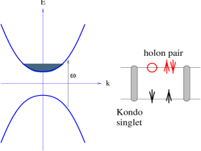
FIG. 1.: Picture of the KLM in strong coupling, with S=1/2. Separation of spin and charge arises. When the hopping amplitude is very small, spin excitations are optical magnons localized on the rungs. The lowest charge excitation consists of (breaking two singlets and) forming a pair of (free) empty and doubly occupied sites with fermionic statistics, as in a Mott insulator at the Luther-Emery point.

A Mott insulator versus Kondo insulator

In a 1D Mott insulator, as a result of commensurability, the charge Hamiltonian is slightly more complicated than the so-called Luttinger Hamiltonian

$${\cal H}_{c}=\frac{u}{2\pi}\int\ dx\ \frac{1}{K}:(\partial_{x}\Phi_{c})^{2}:+K:{(\Pi_{c})}^{2}:,$$ (1)

and contains, in addition to the quadratic part, a Sine-Gordon (SG) umklapp term

$${\cal H}_{um}=\frac{2g_{3\perp}}{(2\pi a)^{2}}\int dx\ \cos\sqrt{8\pi}\Phi_{c}(x).$$ (2)

The displacement field $\Phi_{c}$ and phase field field $\Theta_{c}$ satisfy the usual commutation rules. All interaction effects are taken into account through the velocity $u$ and the Luttinger liquid parameter K (LLP). This obeys $K=1$ in the absence of interactions, $K>1$ for attractive interactions and $K<1$ for repulsive ones. It is convenient to perform the following canonical transformation: $\Phi_{c}\rightarrow\sqrt{K}\Phi_{c}$, $\Pi_{c}\rightarrow\Pi_{c}/\sqrt{K}$. Then, ${\cal H}_{um}$ reads:

$${\cal H}_{um}=\frac{2g_{3\perp}}{(2\pi a)^{2}}\int dx\ \cos\sqrt{8\pi K}\Phi_{c}(x).$$ (3)

The interaction is then absorbed in the argument of the cosine term. For repulsive interactions, this produces a quasiparticle gap $\Delta\propto{g_{3\perp}}^{1/(2-\frac{n^{2}}{4\pi})}$, with $n^{2}=8\pi K$.

A strong (on-site) repulsion between electrons must inevitably result in $K=1/2$ close to half-filling[19, 20]. Then, we start with such bare value of the LLP. Charge degrees of freedom (holons) should behave as spinless fermions[21]. Through the Jordan-Wigner transformation in 1D (Appendix A), one can formally rewrite bosons operators in terms of spinless fermions $(q=\pm)$[8, 9]:

$$\psi_{q}(x)=\frac{\eta_{q}}{\sqrt{2\pi a}}:\exp i\sqrt{\pi}(\Theta_{c}+q\Phi_{c})(x):.$$ (4)

This procedure is called refermionization. Klein factors $\eta_{q}$ are built to fullfill anticommutation rules between left $(-)$ and right $(+)$ movers. More crucially, for $K=1/2$, the SG-umklapp definitely creates fermionic kinks[18]

$$\frac{g_{3\perp}}{(2\pi a)^{2}}\cos\sqrt{4\pi}\Phi_{c} = \frac{\Delta}{2\pi a}\cos\sqrt{4\pi}\Phi_{c}$$ (5)

$$= -i\Delta\hbox{(}\psi_{+}^{{\dagger}}\psi_{-}-\psi_{-}^{{\dagger}}\psi_{+}\hbox{)}.$$ (6)

Klein factors have been chosen as $\eta_{+}\eta_{-}=+i$. The mass term always favors the pinning of the $4k_{F}$ charge-density wave (CDW), producing in our case a Kondo insulator, which is rather characterized by an even number of electrons per unit cell when adding the local moments. The holons disappear from the Kondo ground state. An excited holon from the valence band carries a wave vector $q=2k_{F}$. A pair holon-(anti)holon[22] produces a kink of $2\pi$ in the superfluid phase $\sqrt{\pi}\Theta_{c}$ at $x$, i.e. a kink of 2 in the charge current, that definitely corresponds to a pair of empty and doubly occupied sites with fermionic statistics. Fourier transforming, one finds:

$${\cal H}_{o}=\sum_{k}(uk)qc^{{\dagger}}_{q,k}c_{q,k}+\frac{g_{3\perp}}{2\pi a}\hbox{(}c^{{\dagger}}_{+,k}c_{-,k}+h.c.\hbox{)}$$ (7)

Using a so-called Bogoliubov transformation, this gives us the new energy spectrum:

$$E_{\pm}=\pm\sqrt{{u}^{2}k^{2}+{\Delta}^{2}}.$$ (8)

At half-filling, the umklapp term gives us a semi-conductor picture of two bands. Therefore, to recover the physics of the KLM in the limit $J_{K}/t\gg 1$, we have only to take the quasiparticle gap[16]:

$$\Delta=g_{3\perp}/2\pi a=3J_{K}/4.$$ (9)

Remarkably, charge properties of half-filled KLM’s remain qualitatively unchanged tuning the Kondo interaction from the strong-coupling to the weak-coupling limit (Section III and especially Appendix B).

Here, at low temperatures, the Kondo interaction can be exactly rewritten as an effective umklapp. However, $g_{3\perp}$ (typically the quasiparticle gap) has then a less explicit dependence in $J_{K}$, due to the consequent renormalization of the backward Kondo coupling at half-filling.

B Consequences of doping

To study the influence of hole doping on transport properties, we now shift the chemical potential at the top of the lower subband $(\mu_{ch}=-\Delta)$. We get:

$${\cal H}_{o} = \sum_{k}u_{c}k(a^{{\dagger}}_{+,k}a_{+,k}-a^{{\dagger}}_{-,k}a_{-,k})$$ (10)

$$u_{c} = \frac{\partial E}{\partial k}=\frac{u^{2}k_{c}}{\sqrt{(uk_{c})^{2}+\Delta^{2}}}\cdot$$ (11)

The fermions (holons) $a_{\pm,k}$ now refer to the partially occupied subband and linearizing the band structure near the new Fermi points produces $k_{c}=\pi\delta$ [$\delta=1-n$, being the hole doping].

By doping such a semiconductor, low-energy properties should be well described through a Luttinger liquid Hamiltonian with a velocity $u_{c}\sim\delta/\Delta$ and $K\rightarrow 1/2$. In the 1D KLM below half-filling, such a LL behavior has been checked numerically, for instance, in ref.[23]. This leads to important consequences.

This produces a metallic phase with finite compressibility $\kappa\propto K/u_{c}$ and Drude weight ${\cal D}\propto u_{c}K$ at zero frequency. Very close to half-filling $(u_{c}\propto\delta\rightarrow 0)$, then the Drude weight should vanish continuously (with a dynamical exponent $z=2$[24, 25]) and $\kappa$ diverges as $\delta^{-1}$. A recent Density Matrix Renormalization-Group (DMRG) study has confirmed for large $J_{K}$ parameters and $T=0$, that $\kappa=\chi_{c}$ (charge susceptibility) diverges as $1/\delta$ near half-filling[26]. Moreover, at low temperatures, one then expects an exponential behavior of the d.c. conductivity.

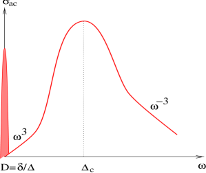
FIG. 2.: a.c. conductivity near the metal-insulator transition induced by doping. In the strong coupling limit $J_{K}/t\gg 1$, the spinless fermion representation of holons or the umklapp-description should remain convenient even at quite high frequency.

The regular part of a.c. conductivity must have two distinct regimes: an $w^{3}$ absorption at small frequency, and a tail $w^{-3}$ at large frequency[17, 27].

To summarize, the commensurate-incommensurate transition of the 1D KLM belongs to the so called Prokovsky-Talapov class of universality[18, 28]. Now, let us push forward the duality with the Hubbard model in the strong $U$-limit, below half-filling.

The model can be mapped onto a Luttinger Hamiltonian as long as $n\neq 1$. Moreover, there is a remarkable duality by exchanging the two parameters $n\leftrightarrow\delta$. Indeed, the parameters $K$ and $u_{c}$ which determine the behavior of the system are known to remain unchanged under the exchange $n\leftrightarrow\delta$[9]. In particular $u_{c}=2t\sin(\pi n)=2t\sin(\pi\delta)$ is the exact velocity of the charge excitations for infinite repulsion[7]. Actually, this implies that there are two equivalent holon representations in the 1D KLM, when $J_{K}\rightarrow+\infty$. First, treating the introduced empty sites as holons leads to a gas of noninteracting spinless fermions in low density $\sim\delta$. As shown precedingly, this picture is particularly accurate to capture transport properties at the commensurate-incommensurate transition. Second, one could also identify the Kondo singlets as holons (single-occupied states would be then localized moments). This produces a gas of noninteracting spinless fermions in large density $\sim n$[29]. This picture has been preferred to show the occurrence of ferromagnetism between unscreened local moments, with an exchange coupling $\sim-t^{2}/J_{K}$[30, 31].

In the pure KLM, the unscreened localized spins polarize completely in order to lower the kinetic energy of mobile holons. Such a case is a concrete application of the Nagaoka’s theorem in 1D. The physics behind this is the finite extension of the screening cloud, which leads to the stability of the ferromagnetic state at finite densities not restricted to the single-electron case.

Note that including an antiferromagnetic Heisenberg exchange $J$ between local moments $J\gg t^{2}/J_{K}$ produces a so-called t-J model and then rather a paramagnet[32].

C Interacting Kinks

Decreasing $J_{K}$ from infinity, results found precedingly on the commensurate-incommensurate transition become now available only for very low doping: Kinks become interacting below half-filling.

Most clearly, a repulsive interaction between the neighboring spinless fermions is introduced in the order of ${\cal O}(t^{2}/J_{K})$[16]. The situation becomes then similar to the infinite $U$ Hubbard model with nearest neighbor repulsion whose $K$ becomes smaller than 1/2[19]. More importantly, the ferromagnetic phase of the pure KLM is very unstable decreasing $J_{K}$ due to the long-range overlap between Kondo singlets resulting in a certain magnetic disorder (see next section). Precisely, a first order phase transition in the intermediate coupling limit from the ferromagnetic state to a paramagnetic one has been pointed out recently[23]. The latter is accompanied by a jump both in the magnetization curve and the value of $K$ (which curiously sharply decreases). This cannot be explained using the preceding analysis.

To conclude: the dependence of $K$ as a function of $J_{K}$ for weaker Kondo couplings remains difficult to handle below half-filling. A general trend, however, is that $K$ is always smaller than 1/3 producing a dominance of $4k_{F}$ charge oscillations, and then a so called Wigner crystal.

III Weak-coupling Kondo transitions

Next, we subsequently stay at half-filling. We explore the perturbative limit, $U/t\ll 1$ and $J_{K}/t\ll 1$. Here, bosonization tricks allow us to explain the occurrence of Kondo insulators in commensurate systems when $J_{K}/t\ll 1$, in a simple way. The small-$J_{K}$ regime is of most interest, since correlation effects (for instance correlations between local moments, or between electrons) are most important there. For this regime, the expansion in $t/J_{K}$ is, of course, not convergent while variational methods are not well controlled. This is mainly because $J_{K}=0$ is a singular limit leading to a metallic behavior. To bosonize the Kondo interaction we need the bosonic representations for the conduction electron- and the localized spin operators. Again, we limit the following study to the case of a single-channel conduction band. In a very general form, that can be used whatever the strength of the Heisenberg interaction J between local moments or their spins S, these are given by[33]:

$$\Psi^{{\dagger}}_{\alpha} (x) \frac{{\sigma}_{\alpha\beta}}{2}\Psi_{\beta}(x)=(\vec{J}_{R}+\vec{J}_{L})$$ (12)

$$+ \frac{e^{2ik_{F}x}}{2\pi a}\hbox{Tr}\{\vec{\sigma}(\Phi^{(1/2)}+\Phi^{(1/2){\dagger}})\}\cos{\sqrt{2\pi}\Phi_{c}}$$ (13)

$$\vec{S}(x) = S\hbox{(}a\vec{L}(x)+(-1)^{x}\sqrt{1-(a{L})^{2}}\vec{N}(x)\hbox{)},$$ (14)

where $|\vec{L}|a\ll 1$ is the quickly varying ferromagnetic component of the local magnetization, and:

$$\vec{L}(x)\cdot\vec{N}(x)=0.$$ (15)

In the weak-coupling limit, fluctuations in the $2k_{F}$ electronic spin operator are produced by the presence both, of doubly occupied and empty sites [for small $U$, holons are described in Appendix B] and of so-called domain walls [spinons of the Heisenberg chain are introduced in Appendix C]. The Hamiltonian for electrons will be also decomposed into a holon part [the same as Eq.(1) with $K=1-Ua/\pi v_{F}$] and the usual spinon part. Moreover, away from half-filling, the continuum limit of the Hamiltonian only contains a marginal Kondo-coupling of the currents[32]:

$${\cal H}_{m}=\lambda_{2}[\vec{J}_{R}+\vec{J}_{L}]\vec{L}(x).$$ (16)

At half-filling, the $2k_{F}$ oscillation becomes commensurate with the alternating localized spin operator and the most prevalent contribution reads:

$${\cal H}_{hf}\propto\lambda_{3}\cos{\sqrt{2\pi}\Phi_{c}}\hbox{Tr}\{\vec{\sigma}(\Phi^{(1/2)}+\Phi^{(1/2){\dagger}})\}\vec{N}(x),$$ (17)

$(\lambda_{2},\lambda_{3})\propto J_{K}$ being the usual forward and backward Kondo scattering processes. Notice the close analogy with the two-chain spin system[34].

A Renormalization-group- and exact treatments

First, it is convenient to use the renormalization group method, expanding in powers of the coupling constant $\lambda_{3}$. The perturbation is divergent, and one can derive renormalization equations upon rescaling of the short distance cut-off $a\rightarrow ae^{l}$:

$$\frac{d\lambda_{3}}{dl}=\hbox{(}\frac{3}{2}-\frac{K}{2}-\Delta_{N}\hbox{)}\lambda_{3},$$ (18)

$\Delta_{N}\leq 1/2$, being in the following the scaling dimension of the localized spin operator (see below, for specific cases).

At half-filling, we expect ${\cal H}_{hf}$ to produce a gap for charge excitations [whatever J or the spin S of local moments]. The charge gap should follow the quasiparticle gap at the Fermi level

$$\Delta\propto\lambda_{3}^{\frac{2}{3-K-2\Delta_{N}}},$$ (19)

for either sign of $\lambda_{3}$. In the weak coupling limit, a Kondo insulator is then formed due to the strong renormalization of the Kondo exchange $\lambda_{3}$.

It should be noted that the exchange coupling $\lambda_{3}$ and the usual umklapp $g_{3\perp}\propto U$ — driven by the on-site Hubbard term — affect the Luttinger parameter $K$ in a symmetric way:

$$\frac{dK}{dl}=-uK^{2}\hbox{(}C_{0}g_{3\perp}^{2}+C_{1}\lambda_{3}^{2}\hbox{)}J_{o}(\delta(l)a).$$ (20)

$J_{o}$ is the Bessel function, and $C_{0}$, $C_{1}$ are constants. At half-filling we must take $J_{o}(0)=1$.

When $\lambda_{3}=0$, the usual umklapp process is known to produce a Mott transition at half-filling. It occurs for a critical value of K which is equal to one, i.e. at the noninteracting point. As soon as $\lambda_{3}\neq 0$, the physics becomes ruled by the Kondo coupling, producing a Kondo transition for a critical Kondo coupling $J_{K}^{c}=0$. The usual umklapp process can be neglected for small $U$ because it (only) scales marginally to strong couplings.

Second, at low temperatures $T\ll\Delta$ the holons, becoming massive, also change of statistics (semions $\rightarrow$ fermions). Charge carriers behave as fermionic kinks due to the strong renormalization of $J_{K}$, and as said before the backward Kondo interaction can be exactly rewritten as an “effective” umklapp process (see Appendix B) — remarkably, whatever $\Delta_{N}\leq 1/2$. The charge gap will have, of course, dramatic consequences for the physical properties. First, this implies a long-range order in the $\Phi_{c}$-field. Indeed, we have to take formally, $K^{*}=0$, for $T\ll\Delta$. Then, at the Kondo transition, there is a finite jump in the compressibility and Drude weight. This will be analyzed in more details in the next section.

B Spin properties for several $\Delta_{N}$’s

Before investigating transport properties in great details, it is maybe appropriate to review several interesting Kondo spin-liquid phases occurring in the weak coupling limit, for particular values of $\Delta_{N}$. Details of the technique can be found in Appendix C.

1 $\Delta_{N}=1/2$: Heisenberg-Kondo lattice for S=1/2

Let us start with the so-called Heisenberg-Kondo lattice, where the spins of the array are coupled through a consequent antiferromagnetic coupling exchange J of the order of t. Here, one can introduce spinon-pairs:

$$\vec{N}=\hbox{Tr}[({\Theta}^{(1/2)}+{{\Theta}^{(1/2){\dagger}}})\vec{\sigma}].$$ (21)

For weak Hubbard interactions (for a parallel, see formula B3), one gets also: $J_{K}<\cos\sqrt{2\pi}\Phi_{c}(x)>\ =\Delta$. Therefore, the backward Kondo interaction is transformed into:

$${\cal H}_{hf}=\Delta\hbox{Tr}{\bf{\Phi}^{(1)}}-3\Delta\epsilon.$$ (22)

By analogy to usual spin ladder systems, the spin spectrum is composed of massive triplet excitations [described by $\hbox{Tr}{\bf{\Phi}^{(1)}}$] with a mass $m_{t}=\Delta$, and of a high-energy singlet branch at $m_{s}=-3\Delta$[35]. We expect the spin gap to decrease for any appreciable difference between J and t.

2 $\Delta_{N}=0$: Weakly coupled S=1/2-local moments

Precisely, let us now study the opposite limit where the local moments are weakly coupled i.e. $J\ll J_{K}$. At short distances, the RKKY interaction — that displays a very small decay in 1D — produces a perfectly static staggered potential with:

$$\vec{N}=\hbox{constant}.$$ (23)

The electrons are then subject to Bragg scattering[36]. This opens a quasiparticle gap (linear in $J_{K}$). On the other hand, these screen away the internal field before a true magnetic transition takes place.

Then, there are still some triplet states in the quasiparticle gap because the SU(2)-spin symmetry is restored at long distances. The resulting spin gap becomes considerably smaller than the charge gap[37].

First, if J is not so far from $J_{K}$, these spin degrees of freedom are described in terms of an O(3) non-linear sigma model without the topological term. The implicit breaking of conformal invariance rescales the spin gap as:

$$\Delta_{S}\propto\Delta\exp-{\pi\hbox{(}\frac{|J-t|}{t}\hbox{)}}\cdot$$ (24)

Single electron excitations in the interval $\Delta_{S}$ and $\Delta$ can be viewed precisely as polarons — i.e. bound states of an electron with a kink of the vector $\vec{N}$[38].

Second, if J tends to 0, the condition for the presence of kink in the local staggered magnetization operator now breaks down. Spin degrees of freedom rather behave as follows[36]. At not too long distances, half of the (electronic) spinon field begins to fluctuate due to the restoration of the SU(2)-symmetry, contributing to a new chiral phase of the same universality class as the 2D Ising model. At long distances, due to strong fluctuations in the spin array, the (electronic) spinon field cannot be pinned anymore by the backward Kondo coupling — i.e. $|\vec{N}|=0$. Then, spin flips should contribute. The system may scale to a perfect singlet ground state at a very low energy scale:

$$\Delta_{S}\propto\Delta\exp-2\pi v_{F}/\lambda_{2}\ll\Delta,$$ (25)

typically the single-site Kondo temperature, in agreement with numerical calculations[16].

To conclude this part: For spin-1/2 local moments, the ground state is always a spin singlet. Furthermore, for small $J_{K}$’s, the antiferromagnetic correlation length is quite large producing disordered quantum fluids. It is already increased by an appreciable difference $(J-t)$, and becomes huge for J=0.

3 $\Delta_{N}=3/8$: Underscreened S=1-chain

Now, we consider another generic case where the local spins form a so-called S=1 Takhtajan-Babujan chain. Details of the calculations can be found in ref.[39]. These can be extended to the case of a spin S-integrable chain $(|1-2S|\neq 0)$ — with $C_{v}/L=2ST/(1+S)$[40, 41].

In the sense of critical theories, this model can be parametrized by a conformal anomaly $C=3/2$. In the continuum limit, this spin-1 chain has then only zero sound triplet excitations — described by three massless Majorana fermions — or rather magnons. The staggered magnetization $\vec{N}$ has now dimension $\Delta_{N}=3/8$. Consult Appendix C3. The Kondo interaction grows to strong coupling, producing a quasiparticle gap $\Delta\propto{J_{K}}^{8/5}$.

Then, a new phenomenon arises: The occurrence of singlet bound states can be achieved only due to the “fractionalization” of each spin triplet excitation onto two spins-1/2. On each rung, (only) one is strongly coupled to the conduction band. This produces the same contribution as in Eq.(22), and then optical magnons in the system. From a general point of view, Luttinger liquids coupled to an active insulating environment via a Kondo-like coupling yield a spin gap[42]. But, deconfined spinon-pairs still subsist in the ground state because the local moments are underscreened. This leads to an anomalous optical conductivity at low frequencies, and then a pseudogap phase. Starting with small J’s (the Haldane gap is irrelevant), predictions from the non-linear sigma model for S=1 give the same conclusion[38].

C Role of electron-electron interactions

The present study shows that the smallest amount of Kondo potential $\lambda_{3}$ produces a Kondo insulator at least for sufficiently large length scales. Then, the backward Kondo scattering can be naturally rewritten as an effective strong umklapp process, such that the original umklapp term — again, driven by the Hubbard interaction — can be neglected.

One can check that the charge gap increases with (enhancing) $U$ — or decreasing the LLP. If the Hubbard repulsion is very large $U/t\gg 1$ one can expect to see a crossover from a Kondo insulator to a usual spin ladder system[34]. Here, the insulating transition should be rather driven by U only, and then we have to take formally $<\cos\sqrt{2\pi}\Phi_{c}(x)>\ =\sqrt{U}=\hbox{constant}$ and $K=0$ in the spin gap equation. For instance, for $\Delta_{N}=1/2$, we recover previous results and for instance the spin gap $\Delta_{s}\propto J_{K}$ (see Appendix C). Another interesting feature is that the Kondo insulating state should even persist in presence of attractive interactions.

A physical mechanism for the generation of attractive interactions is electron-phonon interaction. A renormalization group treatment of the important spin-backscattering term $g_{1\perp}$ (given in Appendix D) predicts, for $J_{K}=0$, the existence of a spin gap

$$\Delta_{ss}\sim\frac{v_{F}}{a}\exp\hbox{(}\frac{-\pi v_{F}}{\left|U\right|a}\hbox{)}\cdot$$ (26)

Remarkably, localization by magnetic impurities remain the most prominent phenomenon as long as $K<K_{c}=3-2\Delta_{N}$. When $K=K_{c}$, the Kondo gap tends to zero and then, a superconducting-like ground state takes place. When $K\geq K_{c}$, correlation functions for the singlet superconducting pairing field are considerably increased in the low-temperature phase $(T\ll\Delta_{ss})$ and the charge sector remains critical, leading to a perfect superfluid. This produces a coexistence between a Luther-Emery liquid and an insulating part characterized by strong antiferromagnetic fluctuations. The pairing also promotes $2k_{F}$ CDW fluctuations that are not sensitive to magnetic impurities.

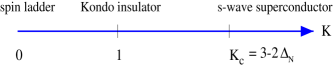
FIG. 3.: The phase diagram as a function of the LLP, $K$. For a large range of $K$ parameters (corresponding to weak $U$’s), the interaction between electrons and magnetic impurities is well prominent, producing a Kondo insulator. For attractive enough interactions $(K>K_{c})$ the electron liquid can turn into a s-wave superconductor decoupling completely from the spin array. A large coherence between spins of the array, resulting in $\Delta_{N}=0,$ tends to increase $K_{c}$.

To conclude: Close to the superconducting transition $(K<K_{c})$, as a remnant of s-wave superconductivity (and CDW fluctuations) one expects that the electron liquid is less localized than for repulsive interactions. Let us now investigate transport properties and comment this point in more details.

IV Transport properties

Transport in such commensurate systems is very interesting because the Kondo process $\lambda_{3}$ provides an important relaxation mechanism for electrons. Next, we will assume that the coupling $\lambda_{3}$ is sufficiently weak that some perturbative calculation of the conductivity as a function of $\lambda_{3}$ can be performed. The conductivity itself does not have a regular expansion in $\lambda_{3}$. A way out is provided by the memory function formalism.

If the system is a normal metal with finite dc-conductivity, one can define[43]

$$\sigma(w)=\frac{2iKu}{\pi}\frac{1}{w+M(w)}\cdot$$ (27)

and $M(w)$ is the meromorphic memory function. This formula is well-suited for an “infinite” system: Next, we are not interested in reservoir effects.

A Memory function approximation

The calculation of this function can be carried out perturbatively to give at the lowest order

$$M(w)=\frac{(\ll F;F\gg_{w}-\ll F;F\gg_{w=0})/w}{-\chi(0)}\cdot$$ (28)

At zero frequency, one gets the retarded current-current correlation function:

$$\chi(0)=-2uK/\pi.$$ (29)

The factor 2 comes from the two colors of spin which both contribute to transport properties. The symbol $\ll;\gg$ designs a retarded correlator computed in the absence of magnetic impurities and $F=[J_{c},H]$, $J_{c}$ is the charge current. The F operators take into account the fact that the charge current is not a conserved quantity.

For frequencies $w\gg M(w)$ and $T\rightarrow 0$, one gets:

$$\sigma_{ac}(w)=\frac{-i\chi(0)}{w}[1-\frac{M(w)}{w}]\cdot$$ (30)

The regular part in the delocalized phase reads:

$$\sigma_{reg}(w)\propto M(w)w^{-2}.$$ (31)

The expression (28) does not necessarily remain valid at very low frequencies, even for finite temperatures. Its validity at low frequencies implicitly assumes in a self-consistent way that the d.c. conductivity behaves as:

$$\sigma_{dc}(T)=\frac{-i\chi(0)}{M(T)},$$ (32)

and $M(T)$ is related to some relaxation time, i.e.

$$M(T)\propto\tau_{rel}^{-1}.$$ (33)

In the macroscopic pure system, one gets $\sigma_{dc}(T)\rightarrow+\infty$. Here, $\tau_{rel}$ should correspond to the effective elastic time between two magnetic diffusions. Of course, it will be highly non-universal and temperature-dependent (since we are in a ballistic transport). This should legitimize the memory function approximation, which gives in general good results as long as we stay far away from an insulating region. This approach, of course, will break down when $T=\Delta$ i.e. when the effect of $\lambda_{3}$ on the ground state becomes strong: it opens a spin- and charge gap changing drastically the nature of the elementary excitations. At low temperatures, the source of large resistance in such magnetic systems comes from prominent quantum scattering which merely destroys the coherence or the propagation of the accelerated preexisting excitations, producing Kondo localization.

Interestingly, here the quantum correlation between spins of the array — driven by $\Delta_{N}$, that plays a crucial role in the classification of the Kondo localizations (e.g. gap equation, spin spectrum), will explicitly appear in the computation of the high-temperature d.c. conductivity. The bosonization scheme gives:

$$J_{c}\sim\sqrt{2}uK\int\Pi_{c}(x)\ dx.$$ (34)

Using the definition of ${\cal H}_{hf}$, the behavior of the memory function as a function of temperature can be easily obtained. We find:

$$\ll T_{\tau}F(\tau)F(0)\gg\ \propto\int dx\ {\lambda_{3}}^{2}{\hbox{(}\frac{1}{x^{2}+(u\tau)^{2}}\hbox{)}}^{\sqrt{1+K+2\Delta_{N}}}\cdot$$ (35)

The function in the integral describes the amplitude that a spinon and a holon recombine to give an electron at the point $x$ and time $\tau$, that is immediately diffused by an impurity. Fourier transforming, one finds:

$$M(w)\propto w^{(K-2+2\Delta_{N})},$$ (36)

and the same behavior as a function of temperature. In the delocalized regime $T\gg\Delta$ or $w\gg\Delta_{c}=2\Delta$, the temperature and frequency dependent conductivity is

$$\sigma_{dc}(T)\propto T^{2-\mu},\sigma_{ac}(w)\propto w^{\mu-4},\mu=K(T)+2\Delta_{N}.$$ (37)

For more details concerning the method, consult ref.[27].

Away from the transition, one may consider the parameter $K(T)$ as a constant $\sim K$. We stress on the fact that dressing of the Kondo exchange by the other interactions results in a nonuniversal power-law dependence in the delocalized regime. Again, the whole perturbative scheme breaks down when $\lambda_{3}\sim 1$, at a length scale which corresponds to the localization length of the system. A reasonable guess of the temperature dependence below this length scale is an exponentially activated conductivity because current-current correlation functions now decrease exponentially in time[44].

As can been seen from Fig.4, there is a maximum in $\sigma_{dc}$ as a function of T for weak attractive interactions $(2-2\Delta_{N}<K<K_{c}=3-2\Delta_{N})$, occurring when the thermal coherence length is of the order in magnitude of the localization length $T\sim\Delta$. This maximum can be well understood as a remnant of s-wave superconductivity in the localized phase that cannot be easily pinned by magnetic impurities. Remind that the system is a very good conductor until one reaches the localization temperature $\sim\Delta$.

A similar phenomenon has been predicted in a disordered two-leg Hubbard ladder system with attractive interactions[45]. In that case, ‘$2k_{F}$’ charge density fluctuations are forbidden due to the spin gap, and ‘$4k_{F}$’ charge density fluctuations, that aim to arise for repulsive interactions, become very small for attractive ones[46]: this is an important consequence of the s-wave scenario in two-leg ladder systems. The nonmagnetic disorder can become efficient only at very low energy. For a comparison with the single Hubbard chain problem, see next subsection.

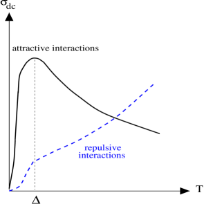
FIG. 4.: The behavior of d.c. conductivity as a function of temperature, for repulsive and for attractive interactions. For $T\gg\Delta$, $\sigma\propto T^{2-K-2\Delta_{N}}$: For repulsive (electron-electron) interactions, there is no maximum in the conductivity and therefore no rest of original umklapps driven by the Hubbard interaction. When the interactions become attractive, the spin density fluctuations are suddenly lowered making the system less localized by magnetic impurities than for the repulsive counterpart.

For repulsive interactions, we can check that there is no remnant of the original umklapp term — again, driven by the Hubbard interaction — which is known to produce $\sigma_{dc}\propto T^{-1}$ (with $K\sim 1$) in the delocalized regime, and then a maximum in $\sigma_{dc}$ in the entrance of the localized phase. In the case of electron-electron interactions, the relaxation time should result from the coupling of electrons with a thermal bath which, strictly speaking, is needed for the system to reach thermal equilibrium[47]. In such case, the relaxation time is rather associated to phase-breaking or inelastic processes[27]. In particular, note that $\sigma_{dc}\equiv\tau_{in}$ (see Appendix D). Furthermore, as long as a spinon is not scattered (as it is the case in the absence of impurities), it may combine locally with another holon to form an electron and the material is still a very good conductor. This is a consequence of spin-charge separation[20].

Most clearly, for repulsive interactions, the ground state of the Hubbard chain is almost a spin-density wave (SDW) (with a power-law decay of the correlation functions) whose charge density is uniform. Such a ground state couples very strongly to magnetic impurities leading to prominent elastic processes in the electron liquid. It is therefore not surprising that for repulsive interactions the main source of resistance for the electron liquid is due to the prominent scattering of a pair spinon-holon (electron) by a magnetic impurity.

Furthermore, the conductivity is found to decrease monotonically with temperature, even at high temperature. This noteworthy renormalization of exponents and the faster decay of the conductivity for repulsive interactions is a perfect signature of Kondo localization. Again, note the nonuniversality of exponents due to the factor $\Delta_{N}$ which depends on the spin S of local moments and on the strength of the Heisenberg interaction between them. To summarize the main point: Now, we are really able to allege that for repulsive interactions the electron liquid is more localized by the magnetic impurities than for attractive interactions, both because of the scale of localization and because of the d.c. conductivity temperature dependence.

B Duality to an effective Gaussian disorder

It should be noted that these results can be reproduced defining the (Kubo) d.c. conductivity as:

$$\sigma_{dc}(T)\sim T^{-1}/D_{m}(T)\hskip 8.5359pt\hbox{and}\hskip 8.5359ptD_{m}(T)={\lambda_{3}(T)}^{2}.$$ (38)

$n(T)=1/T$ denotes the electronic density at a temperature T. We must stop renormalization procedure at the thermal length $L=l_{in}=v_{F}/T$ at which inelastic and decoherent effects take place. By comparison with the case of a nonmagnetic Gaussian disorder[14],

$$D_{m}(T)=l_{in}/l_{e}\propto T^{-(3-\mu)}.$$ (39)

The exponent $\mu$ has been defined in Eq.(37). In KLM’s, $D_{m}$ will be identified as the magnetic disorder parameter. For more details, consult Appendix D. This definition traduces that at high temperatures we have a perfect duality to a model of a 1D electron liquid submitted to a Gaussian correlated spin disorder, with an effective exponent $\mu=K(T)+2\Delta_{N}$ for the electronic spin density-spin density correlation function. In the case of a Gaussian correlated nonmagnetic disorder, for SU(2) symmetry and repulsive interactions one rather expects[48, 49]:

$$\sigma_{dc}(T)\propto T^{2-\hat{\mu}}\hskip 8.5359pt\hbox{with}\hskip 8.5359pt\hat{\mu}=1+K(T).$$ (40)

Far away from the localization energy scale i.e. for very small disorder, one can take $\hat{\mu}=1+K$[50]. Note that to couple to nonmagnetic disorder one has to distort the SDW and make a fluctuation of the charge density, a process which costs an energy of order U. Therefore, for repulsive interactions, the non-magnetic disorder effect must be inevitably weaker than for attractive interactions where $2k_{F}$ CDW fluctuations can get very easily pinned by nonmagnetic impurities. Starting with the Hubbard model and small U, the d.c. conductivity found above is then not completely correct. The reason is that the backscattering spin term $g_{1\perp}$ couples to the non-magnetic disorder, and then it cannot be ignored (see Appendix D). At intermediate length scales, this results rather in:

$$\sigma_{dc}(T)\propto T^{-Ua/\pi v_{F}}.$$ (41)

Now, the maximum in the d.c. conductivity in the entrance of the Anderson glass phase occurs for repulsive interactions. The situation becomes opposite to that found with an array of magnetic impurities.

In general, for repulsive interactions one gets $\mu<\hat{\mu}$, revealing that Kondo localizations may still take place in weakly disordered 1D Kondo lattice models. Especially when $\Delta_{N}=0$, we have a constant uniaxial Kondo potential at high temperatures

$$\overline{V(x)}=\lambda_{3},\qquad\overline{V(x)V(0)}=D_{m},$$ (42)

and $\mu=K(T)\ll\hat{\mu}$. There is no quantum fluctuation. The long-range coherence of the spin array produces inevitably Kondo localization. On the other hand, adding explicitly a dominant antiferromagnetic direct exchange between local moments should produce a stronger competition between Anderson- and Kondo localizations, even if the ground state is always of Kondo type for prominent repulsive interactions[51]. This comes from the facts that $2k_{F}$ CDW fluctuations are not completely forbidden at high temperatures for weak on-site repulsive interactions, and that the Kondo potential follows:

$$\overline{V(x)}=0,\qquad\overline{V(x)V(0)}=D_{m}/x^{2\Delta_{N}}.$$ (43)

It is now short-range correlated, and we have $\Delta_{N}=3/8$ (Takhtajan-Babujan S=1 chain), or $\Delta_{N}=1/2$ (Heisenberg S=1/2 chain). The average is explicitly performed on quantum fluctuations (after normal ordering). Below, we will investigate the case of a Gaussian correlated magnetic disorder (subsection E): again it will lead to the same conclusion. Using Appendix D, one can easily check that repulsive interactions tend to make the nonmagnetic disorder less relevant and decrease localization. This has dramatic consequences on the effects of interactions on persistent currents[52]. Comparisons with the renormalization of charge stiffness in 1D KLM’s will be made later in subsection D.

C Charge incompressibility with $\sigma(w,k=\pi)\neq 0$

In the following, we present a new class of Kondo insulators which is (charge) incompressible, but yields only a pseudo gap in the (charge) optical conductivity at a large wave-vector $k=\pi$.

On the one hand, the Kondo transition at half-filling produces an incompressible system because $\kappa\propto K^{*}=0$. On the other hand, ordinary Kondo insulators [where local moments are characterized by $S=1/2$] have no charge conductivity for low frequencies. First, the charge current $J_{c}$ given by the expression (34) vanishes. Second, the presence of a spin gap in the system produces optical magnons, that doesnot allow any anomalous charge current at large wave-vectors (see Appendix C).

Now, let us investigate the case where local moments form a Takhtajan-Babujan S=1 chain. As shown precedingly, free spinons remain in the ground state of the system due to the ‘underscreening’ of the local impurities. This implies that the optical charge-conductivity would reveal no gap at low frequency and $k=\pi$.

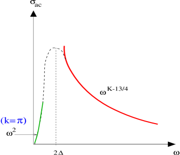
FIG. 5.: The behavior of a.c. conductivity at zero temperature as a function of frequency in the case of a Takhtajan-Babujan chain i.e. $\Delta_{N}=3/8$. Conversely to usual Kondo insulators, $\sigma_{ac}(w,k=\pi)\propto{w}^{2}$ for vanishing frequencies. This is a nice example of pseudo-gap phase.

Spinons are governed by an extra term in the action [we use the duality: $\Phi^{(1/2)}=i\vec{\sigma}{\bf\Phi}$],

$$\Gamma(i\vec{\sigma}{\mathbf{\Phi}})=\frac{i}{8\pi}\int dxd\tau\ \epsilon_{\mu\nu}\hbox{(}{\mathbf{\Phi}}\cdot[\partial_{\mu}{\mathbf{\Phi}}\times\partial_{\nu}{\mathbf{\Phi}}]\hbox{)}=i\pi Q$$ (44)

where $Q=1=\int dx\ q(x)$ is the associated topological charge. From this (topological) charge, one can define an anomalous current density[38],

$$\bar{\psi}(i\sigma^{z})\psi={\cal J}_{S}=\epsilon_{\mu\nu}\hbox{(}{\mathbf{\Phi}}\cdot[\partial_{\mu}{\mathbf{\Phi}}\times\partial_{\nu}{\mathbf{\Phi}}]\hbox{)},$$ (45)

which has the scaling dimension 5/2. In this way, the charge- and the spin sector are related to each other. Then, the pair correlation function of $J_{S}$ induces an unusual feature in the optical conductivity at a large wave-vector $k=\pi$. The anomalous current is nothing but the ordinary current at $k=\pi$. We find a retarded current-current correlation function $\chi(w)\sim-iw^{3}$ and then an optical conductivity,

$$\sigma(w,k=\pi)=\frac{i}{w}\chi(w)\propto w^{2}.$$ (46)

We obtain a new class of incompressible Kondo systems, with no gap in the optical conductivity (Fig.5). Similar conclusions can be reached in the case where the direct exchange between local moments is very weak[38].

It should be noticed that a new phase of disordered commensurate insulators yielding “similar” features, has been pointed out recently[53]. The corresponding phase with $\kappa=0$ and $\sigma(w,k=0)\propto w^{2}$ results from a strong competition between Mott- and Anderson localization which leads to unusual excitonic effects. This requires some interactions of finite extent.

D Renormalization of the Drude peak

In addition to the regular frequency dependence of the a.c. conductivity found precedingly, one can compute the charge stiffness ${\cal D}$ of the macroscopic system, which measures the strength of the Drude peak (occurring at zero frequency):

$$\sigma_{ac}(w)={\cal D}\delta(w)+\sigma_{reg}(w).$$ (47)

This comes from the first term in Eq.(30). For fermions with spins, the conductivity stiffness at length $l$ can be obtained using:

$${\cal D}(l)=2u(l)K(l),$$ (48)

with ${\cal D}(l=0)=2uK=2v_{F}$. Again the factor of two comes from the fact that there are twice degrees of freedom compared to the spinless fermionic case. The velocity $u$ obeys a recursion law of the type:

$$\frac{du}{dl}=-C_{2}u^{2}KD_{m}(l).$$ (49)

$C_{2}$ is a constant. From Eqs.(20),(49) one can easily obtain the renormalization group equation for ${\cal D}$:

$$\frac{d{\cal D}}{dl}=-CD_{m}(l),$$ (50)

and C is a constant. Using the flow of $D_{m}(l)$ given explicitly in Appendix D, one obtains:

$$\frac{d{\cal D}}{dl}=-CD_{m}(0)e^{(3-\mu)l}.$$ (51)

By stopping the renormalization procedure at a length $L=e^{l}=v_{F}/T$, it follows:

$${\cal D}(L)-{\cal D}(1)=-C\frac{D_{m}(1)}{(3-\mu)}\hbox{[}L^{(3-\mu)}-1\hbox{]}.$$ (52)

We can notice that for repulsive interactions the Drude peak fastly decreases with $L$, that is also typical of a Kondo localization. For attractive interactions, the Drude peak decreases more slowly and the renormalization of ${\cal D}$ stops completely as soon as $\mu=3$ that coincides with $K=K_{c}$. This is in agreement with the fact that for $K\geq K_{c}$ the system behaves as a perfect superfluid at low energy. In the localized phase $(T\ll\Delta)$, the opening of the gap produces formally $K^{*}=0$ and then the Drude weight vanishes. Using Eq.(52) for $L\rightarrow{\Delta}^{-1}$, one can therefore deduce that there is (also) a jump in the Drude weight at the transition. Using ref.[25] and replacing $\delta$ by $(T-\Delta)$, one then finds that the dynamical exponent is $z=1$, that is specific of a Kosterlitz-Thouless transition. Again note the close parallel with the calculation of the charge stiffness in presence of a Gaussian disorder[52]:

$${\cal D}(L)-{\cal D}(1)=-\hat{C}\frac{D(1)}{(3-\hat{\mu})}\hbox{[}L^{(3-\hat{\mu})}-1\hbox{]}.$$ (53)

Nonetheless, physical consequences are very different. For small U one gets:

$$(3-\hat{\mu})=1-\frac{Ua}{\pi v_{F}}\cdot$$ (54)

For finite non-magnetic disorder, one finds that the charge stiffness of the system for repulsive interactions is larger than the one of the system for attractive interactions. Again, SDW fluctuations that are prominent for repulsive interactions tend to make the quenched disorder less relevant and decrease localization. The charge density tends to be rather homogeneous. Conversely, for attractive interactions, $2k_{F}$ CDW fluctuations can get very easily immobilized by non-magnetic impurities.

E Randomly distributed magnetic defects

For completeness, we now make links with the case where magnetic impurities would be randomly distributed. To simplify at maximum the discussion, we consider here that these exercise a unixial random magnetic field along the z-axis. One gets the Hamiltonian (see Appendix D):

$$H_{m.dis}=\int dx\ V(x)\cdot\rho_{s}^{z}(x),$$ (55)

$V(x)$ (complex) is assumed to be Gaussian correlated, resulting in

$$\overline{V(x)}=0,\qquad\overline{V^{*}(x)V(0)}=D_{m}\delta(x).$$ (56)

The forward scattering potential, that does not affect transport properties, will be omitted. Now, we apply standard renormalization-group methods for one-dimensional disordered systems[48]. In the Abelian representation, the random Kondo potential reads:

$$H_{m.dis}=\int dx\ V(x)\sin{\sqrt{2\pi}\Phi_{s}(x)}\cos{\sqrt{2\pi}\Phi_{c}(x)}.$$ (57)

Here, random magnetic impurities are not explicitly linked to each other (the Kondo potential is ‘on-site’ correlated). Now, we show that preceding conclusions remain unchanged: The electron liquid is more localized by magnetic impurities for repulsive interactions than for attractive ones. We follow exactly the same scheme as in Appendix A of ref.[48]. From a perturbative expansion in the magnetic disorder parameter $D_{m}$ and the spin backscattering $g_{1\perp}$, the result is:

$$\frac{dD_{m}}{d\ln T}=-(3-K_{s}-K+\frac{g_{1\perp}}{\pi v_{F}})D_{m}.$$ (58)

The main difference with non-magnetic disorder comes from the sign (plus and not minus) of the last term, coupling interactions and Kondo potential. This is because electronic spin degrees of freedom are linked to the random field via a sinus term (and not a cosine). For a simple sight, consult Appendix E. As a consequence, we still have a strong competition between localization of the electron liquid by (disordered) magnetic potential and superconductivity: For $g_{1\perp}\rightarrow-\infty$, the flow of $D_{m}$ scales to zero. For small U, one finds:

$$\frac{dD_{m}}{d\ln L}=(1+\frac{Ua}{\pi v_{F}})D_{m}.$$ (59)

and,

$$\frac{dK}{dl} = -C_{1}uK^{2}D_{m},$$ (60)

$$\frac{dK_{s}}{dl} = -C_{3}{K_{s}}^{2}D_{m}.$$ (61)

$C_{3}$ is a constant. In the infra-red region, quantum coherence between impurities definitely appears and then $K^{*}$ and $K_{s}^{*}$ approach zero. The spin backscattering term $g_{1\perp}$ remains small. Furthermore, the $2k_{F}$ electronic spin density wave will be weakly pinned by the random magnetic field — induced by local moments — resulting in a glassy- and presumably a disordered Ising phase[54].

Far in the delocalized regime, one can equate the exponent $\mu$ to $1+K$. The result is then:

$$\sigma_{dc}\propto T^{Ua/\pi v_{F}}.$$ (62)

At short length scales, the impurities can be considered as independent (see next section). One can also notice the close correspondence with the so-called Heisenberg-Kondo lattice model with $\Delta_{N}=1/2$. This fact certainly traduces that in the delocalized regime there is no fundamental difference between on-site- and (very) short-range correlated Kondo potentials. Likewise, a maximum in the d.c. conductivity curve again should take place in the entrance of the Kondo (glass) phase for attractive interactions. For an explicit comparison with non-magnetic impurities, consult Eq.(41). Finally, one can also check that repulsive interactions help in reducing the conductivity stiffness, while attractive interactions reduce the decrease of conductivity stiffness by magnetic disorder

$${\cal D}(L)-{\cal D}(1)=-C\frac{D_{m}(1)}{(3-\mu)}\hbox{[}L^{(1+\frac{Ua}{\pi v_{F}})}-1\hbox{]}.$$ (63)

On the other hand, the stiffness ${\cal D}$ generally provides a nice measure of the persistent current in a mesoscopic ring induced by a small magnetic flux[55]. Therefore, the above results could have some applications in nearly one-dimensional mesoscopic rings (of size L: The electron has to stay coherent along the whole ring) with prominent magnetic defects: for example, repulsive interactions should decrease persistent currents. Extensions of such model will be considered elsewhere.

V Links with the single impurity case

Let us now compare with the case of a single magnetic impurity in a Luttinger liquid. At half-filling, here usual umklapps produce an Heisenberg chain. The resulting Kondo effect has been studied in ref.[56]. Away from half-filling, the Kondo interaction gives the same two contributions as in Eqs.(16),(17) [forward and backward scatterings]. Since scattering occurs only on a finite part of the sample, the conductance is the most appropriate way to describe transport.

A New renormalization flow

For weak $J_{K}$’s, one can use the same renormalization method expanding in the interactions $\lambda_{2}$ and $\lambda_{3}$. One obtains the RG equations

$$\frac{dK}{dl} = 0$$ (64)

$$\frac{d\lambda_{2}}{dl} = \frac{1}{2\pi v_{F}}{\lambda_{2}}^{2}+\frac{K}{2\pi v_{F}}{\lambda_{3}}^{2}$$ (65)

$$\frac{d\lambda_{3}}{dl} = \frac{1}{2}(1-K)\lambda_{3}+\frac{1}{\pi v_{F}}\lambda_{2}\lambda_{3}.$$ (66)

First, note that the first term in the third equation is seemingly different from the one for the lattice case: it comes from the fact that the impurity only acts at $x=0$, leaving only a double integral over time and producing $\Delta_{N}=0$. The single-impurity gap (or the single-site Kondo temperature) now scales as

$$\Delta\propto{\lambda_{3}}^{\frac{2}{1-K}}\equiv{\lambda_{3}}^{\frac{2\pi v_{F}}{U}}.$$ (67)

For $U\rightarrow 0$, marginal operators produce the usual Kondo temperature [identical to Eq.(25)]. The second difference compared to the finite density of impurities is the absence of renormalization of the bulk exponent $K$, which clearly displays that there is no source of Drude resistivity (nor scattering effects) far away from the impurity spin. Thus, the two $\beta$-functions (for $\lambda_{2}$ and $\lambda_{3}$, respectively) become strongly coupled due to the presence of the extra term ${\cal O}({\lambda_{3}}^{2})$ in the second equation. To show the existence of such a term, one can for instance utilize current algebera techniques for the operators[57]. The charge field satisfies the operator product expansion (OPE) of a U(1) Gaussian model,

$$:\exp(i\sqrt{2\pi}\Phi_{c}(\tau))::\exp(-i\sqrt{2\pi}\Phi_{c}(0)):\ \propto\frac{1}{u\left|\tau\right|^{K}}\cdot$$ (68)

One can also use the OPE of spinon pairs:

$$\hbox{Tr}[\Phi^{(1/2)}(\tau){\sigma}^{a}]\cdot\hbox{Tr}[\Phi^{(1/2)}(0){\sigma}^{b}]\propto i\epsilon^{abc}[J_{L}^{c}+J_{R}^{c}].$$ (69)

All these operators act on $x=0$, and $\tau$ is close to 0. The local impurity spin obeys a usual SU(2) Lie algebra:

$$[S^{a},S^{b}]=i\epsilon^{abc}S^{c}.$$ (70)

Exploiting Eqs.(68),(69) and (70) and the fact that $\left|\tau\right|^{K}\sim dl$, one inevitably finds the extra term in the second equation. We have also applied the equality $uK=v_{F}$, from the LL theory in presence of Galilean invariance (Appendix A). Let us insist on the fact that in the KLM at half-filling the exponent $K^{*}$ tends to zero at low temperatures so that forward and backward Kondo exchanges are independent also in the infra-red region. It is not the case in the single impurity case; the low-temperature behavior is well controlled by $\lambda_{2}=\lambda_{3}\rightarrow+\infty$.

B Transport and fixed points

At high temperatures, the only effect of the interaction $\lambda_{3}$ is therefore to change the Born amplitude of magnetic scattering. The conductance is given by the effective scattering at the scale $L=\exp l\sim 1/T$. Integrating out (64), one gets a Landauer-type conductance:

$$G_{0}-G(T)=-\delta G(T)\propto{\cal R}(T)=D_{m}^{o}T^{\tilde{\mu}-2},$$ (71)

with:

$$\tilde{\mu}=K+1.$$ (72)

$G_{0}=2e^{2}K/h$ is the conductance of the pure wire (again, without any reservoir-effect). Applying a generalized Fermi Golden’s rule at $T\neq 0$, one can check that ${\cal R}(T)\sim D_{m}^{o}(T)={\lambda_{3}(T)}^{2}$ is the resistance produced by a sole impurity. It obeys:

$$\frac{dD_{m}^{o}}{dl}=(2-\tilde{\mu})D_{m}^{o}.$$ (73)

This produces the same thermal laws as a pointlike nonmagnetic defect at $x=0$ (see, for instance[14] and references therein), i.e.

$$G_{0}-G(T)\propto T^{K-1}.$$ (74)

On the one hand, attractive interactions $(K>1)$ favor the formation of singlet superconducting pairs that can completely suppress the back flow at zero temperature. Here, the impurity becomes unscreened for “vanishing” attractive interactions or at least as soon as $U>J_{K}$. In comparison, remember that the coherence between localized spins in the lattice problem should prevent a superconducting-like ground state until attractive enough electron-electron interactions, i.e. $K\geq K_{c}=3-2\Delta_{N}$. Furthermore, the Drude weight or superfluid stiffness is already large in the weak attractive patch $(\sim 2v_{F})$.

One the other hand, if the backward and forward Kondo couplings are relevant i.e. for $K<1$, the weak coupling renormalization group scheme ceases to be valid as soon as the Born amplitude ${\lambda_{3}}^{2}$ is of order one (i.e. for $T\sim\Delta$). From Eq.(67) one can notice that the single-site Kondo temperature is substantially enhanced by the strong repulsive interactions in the 1D LL: Again, repulsive interactions promote SDW fluctuations in the electron liquid that interact prominently with the localized impurity. The screening of the impurity becomes prominent and we have the formation of a strong nonmagnetic barrier at $x=0$. The fact that $\lambda_{3}$ flows to strong couplings produces a new boundary condition at the origin:

$$<\Phi_{c}(0)>\ =\sqrt{\frac{\pi}{2}}\ \leftrightarrow\ <\chi^{{\dagger}}_{-}(0)\chi_{+}(0)>\ =\sqrt{\Delta},$$ (75)

that pins the charge cosine potential. The impurity is screened by a physical electron and then holons now escape away from the impurity site (see Appendix B): no kink in $\Phi_{c}$ is then possible at the origin. By symmetry, two different fixed points are authorized.

First, one can consider weak tunneling of electrons through the impurity site. This fixed point has been analyzed in refs.[58, 59] and still gives a power law for the conductance, but with a different exponent than in the weak coupling limit:

$$G(T)\propto T^{1/K-1}.$$ (76)

Of course, it vanishes at zero temperature. The exponent $\tilde{\mu}$ is renormalized as:

$$\tilde{\mu}=1+1/K.$$ (77)

In such case, backscattering off magnetic impurity will tend to reduce considerably the current in the wire. From this point of view, we obtain a perfect insulator at $T=0$: However, in the single impurity case the d.c. conductivity still grows at low temperatures [see Eqs.(34),(76)]. Since $K$ does not change with $l$, the transition between zero/finite conductance here occurs at $\tilde{\mu}=2$, i.e. in the neighborood of the noninteracting fixed point $K_{c}=1$. This situation would require that the screening characteristic time is very large compared to the tunneling one.

Second, one could rather investigate the opposite limit [i.e. screening time $\ll$ tunneling time]. By extension of the noninteracting case, one could then expect a nonperturbative ground state of Fermi liquid type. Using boundary conformal field theory, we have proved that electron-electron interactions could also produce another ground state with typically the same thermodynamic properties as a 1D Fermi liquid, but with “magnon” spin quasiparticles and a nonuniversal Wilson ratio[59].

Numerical works are up to now not very numerous: A recent DMRG study[60] and a quantum Monte-Carlo procedure[61] have both checked that the impurity is well screened at low temperatures and found for very large Hubbard interactions, a susceptibility law $\chi(T)\sim 1/\Delta$, typical of a heavy Fermi liquid. In such limit, charge degrees of freedom are completely frozen and the unusual power law behavior predicted in ref.[58, 59] cannot arise anymore. This scenario maybe could help in describing the recent heavy-fermion behavior reported in the strongly correlated (two-dimensional) material $Nd_{2-x}Ce_{x}CuO_{4}$[62]. Furthermore, computing the susceptibility curve at low temperatures, the authors of ref.[61] have reported a non-Fermi liquid behavior with an anomalous exponent $\eta=1/K$[58, 63] for weak interactions, and a Fermi-liquid exponent $\eta=2$ for vanishing interactions.

The fact that a simultaneous existence of two leading irrelevant operators, one describing Fermi-liquid behavior and the other describing Furusaki-Nagaosa anomalous behavior [implying: screening time $\simeq$ tunneling time], should not be possible for weak interactions would deserve further numerical works.

A summary of the various equations and transport properties for the Kondo lattice(s) and the single impurity case is given in table 1.

C Array of independent impurities

To achieve this part, let us briefly compare with the case of $N_{i}={\cal L}/a$ independent magnetic impurities in a wire of length $L={\cal L}$ (i.e. the density of magnetic impurities is fixed to $n_{i}=1$). The total resistance of the wire reads

$${\cal R}_{tot}(T)=\sum_{N_{i}}\ D_{m}^{o}(T)=\frac{{\cal L}}{a}D_{m}^{o}(T)\neq D_{m}(T).$$ (78)

Now, using the precious link between conductance and conductivity in 1D for a metallic system of size ${\cal L}$,

$$G_{tot}={\cal L}^{-1}\sigma_{dc},$$ (79)

one finds the high-temperature law:

$$\sigma_{dc}(T)\propto{\cal L}{\cal R}_{tot}^{-1}=a[D_{m}^{o}(T)]^{-1}\propto\frac{1}{D_{m}^{o}}T^{1-K}.$$ (80)

In the preceding studies of the Kondo lattices, we have obtained the same formula replacing $\tilde{\mu}$ by $\mu$. Since $\mu\ll\tilde{\mu}$ [because $\Delta_{N}\leq 1/2$ and especially because $K(T)$ becomes smaller and smaller decreasing the temperature in the real lattice problem], this leads to a faster decay of conductivity/conductance when the temperature decreases, compared to that of independent magnetic impurities. Coherent effects between magnetic impurities are included through the scaling dimension parameter $\Delta_{N}$, and through the quantum renormalization of the exponent $K$, as well. These definitely enhance Kondo localization. Likewise, note that when the impurities are supposed to be completely independent, localization should not occur for attractive interactions [see Eq.(73)].

VI Conclusion

To summarize, we have studied (two) metal-Kondo insulating transitions possibly occurring in one dimensional quantum wires. These result from a consequent antiferromagnetic (Kondo) coupling between conduction electrons very close to half-filling and a perfect lattice of local moments — producing a usual KLM.

As a result of commensurability, we have shown how a one-dimensional Kondo insulator can be understood as an effective (strong) umklapp process becoming relevant. Therefore, studying the pure KLM in the strong Kondo coupling limit $J_{K}\gg t$, results in a commensurate-incommensurate transition of Pokrovsky-Talapov type at zero temperature. For instance, the charge susceptibility should diverge as the inverse of the doping near half-filling, that is in good agreement with recent numerical datas[26].

In the weak coupling region $(J_{K},U)\ll t$, Kondo transitions can be classified as a function of the coherence-parameter in the spin array i.e. the scaling dimension of the staggered magnetization operator, namely $\Delta_{N}$, which is always smaller than 1/2. These arise due to the important renormalization of the backward Kondo potential. In such regime, the interplay between electron-electron interactions and backward Kondo scattering is predicted to produce exotic and fascinating features in transport properties, in the high-temperature (ballistic) regime — whatever $\Delta_{N}\leq 1/2$.

For repulsive interactions, the conductivity is found to decrease monotonically with temperature — even at high temperature: There is no remnant of the original umklapp process driven by the on-site Hubbard interaction. The resulting Kondo insulating phases are still stable in presence of weak non-magnetic disorder. These are perfect signatures of Kondo localizations.

In contrast, for weak attractive interactions, the electron liquid is less localized by magnetic impurities, and then the d.c. conductivity yields a maximum in the entrance of the localized phase. This is a precursor of the s-wave superconducting phase occurring for stronger attractive interactions.

The Kondo localization should even persist when the impurities are supposed to be randomly distributed. In particular, repulsive interactions also help in reducing the conductivity stiffness at intermediate length scales. As a consequence, persistent currents on thin mesoscopic rings with prominent magnetic defects should then decrease for repulsive interactions.

Finally, for completeness, consequences of the backward Kondo scattering on transport of LL’s have been summarized in Table 1, both in the one impurity case and that of a perfect lattice of magnetic impurities.

A Duality spinless fermion-boson in one dimension

We use a continuum version of the Jordan-Wigner scheme to rewrite the right and left electron fields $\Psi_{q}(x)$ (with $q=\pm$) in a bosonic basis. We define

$$\Psi(x)=\Psi_{+}(x)+\Psi_{-}(x).$$ (A1)

and,

$$\psi_{j}\rightarrow\Psi(x)\sqrt{a}$$ (A2)

$a$ being the lattice spacing. Each fermion operator can be re-expressed as,

$$\Psi_{q}(x)=\frac{1}{\sqrt{2}}{\cal O}_{q}(x){\cal B}(x)=\frac{1}{\sqrt{2}}\exp[i\pi q\sum_{y<x}n(y)]{\cal B}(x),$$ (A3)

where $n(x)=\sum_{q}\ \Psi_{q}^{{\dagger}}(x)\Psi_{q}(x)$ is the total number operator, and ${\cal B}(x)$ is in principle an explicit hard core boson operator. The extra factor $1/\sqrt{2}$ allows to fullfill the Jordan-Wigner constraint,

$$n(x)={\cal B}^{{\dagger}}(x){\cal B}(x).$$ (A4)

By construction of spinless fermions, we have: ${\cal B}^{2}(x)=0$. On the other hand, as long as $\left|x-y\right|\geq 1$ (1 being now the lattice spacing), we can check that Bose operators always commute. The trick is then to come back to a free boson system using the argument that in very low density there is no real difference between free- and hard core bosons. To perform this explicitly, we rewrite

$$n(x)=\rho_{o}+b^{{\dagger}}(x)b(x),\ \rho_{o}=\frac{1}{2}=\frac{k_{F}}{\pi}\cdot$$ (A5)

Considering a gas of spinless fermions near half-filling $[n(x)\rightarrow 1/2]$ results in:

$$\frac{\delta\rho}{\pi}=b^{{\dagger}}(x)b(x)\rightarrow 0,$$ (A6)

and approximately,

$$b(x)=(\frac{\delta\rho}{\pi})^{1/2}\exp i\sqrt{\pi}\Theta_{c}.$$ (A7)

$\delta\rho$ measures density fluctuations and $\Theta_{c}$ is the associated superfluid phase. This corresponds to the usual phase-amplitude decomposition. It is convenient to introduce a phonon-like displacement field:

$$\delta\rho(x)=\sqrt{\pi}\partial_{x}\Phi_{c}(x).$$ (A8)

As usual, the density and phase are canonically conjugate quantum variables taken to satisfy:

$$[\Theta_{c}(x),\partial_{y}\Phi_{c}(y)]=i\delta(x-y).$$ (A9)

This choice of wave-function is particularly judicious because it satisfies the (last) condition that $\Psi_{q}(x)$ must remove a unit charge e at the coordinate x. To see this, one can rewrite:

$$e^{i\sqrt{\pi}\Theta_{c}}=e^{i\sqrt{\pi}\int_{-\infty}^{x}\ dx^{\prime}\ \Pi_{c}(x^{\prime})},$$ (A10)

and

$$\Pi_{c}=\partial_{x}\Theta_{c},$$ (A11)

is the momentum conjugate to $\Phi_{c}$. Since $\Pi_{c}$ is the generator of translations in $\Phi_{c}$, this creates a kink in $\Phi_{c}$ of height $\sqrt{\pi}$ centered at $x$, which corresponds to a localized unit of charge using the definition of $b^{{\dagger}}(x)b(x)$. Moreover, the Jordan-Wigner string can be rewritten:

$${\cal O}_{q} = \frac{1}{\sqrt{2}}\exp iq\int^{x}\ dx^{\prime}\ (\delta\rho(x^{\prime})+k_{F})$$ (A12)

$$= \frac{1}{\sqrt{2}}\exp iq(k_{F}x+\sqrt{\pi}\Phi_{c}(x)).$$ (A13)

We have thereby identified the correct Bosonized form for the (continuum) electron operators:

$$\Psi(x)=\psi_{R}(x)e^{ik_{F}x}+\psi_{L}(x)e^{-ik_{F}x},$$ (A14)

with:

$$\psi_{q}=\frac{\eta_{q}}{\sqrt{{2}\pi a}}:\exp i\sqrt{\pi}(\Theta_{c}+q\Phi_{c}):.$$ (A15)

We have replaced the lattice step $a$ taken to satisfy Eq.(A3). This construction has been built originally by Haldane. The expression (A13) is called normal ordered (: :) meaning that all $\infty$ constants have been substracted from the fermionic ground state. In particular, we have:

$$\sum_{q}\psi_{q}^{{\dagger}}(x)\psi_{q}(x)\propto\partial_{x}\Phi_{c}(x)\rightarrow 0.$$ (A16)

We have added Klein factors defined by ${\eta_{-}}^{2}={\eta_{+}}^{2}=1$ and ${\eta_{+}}{\eta_{-}}+{\eta_{-}}{\eta_{+}}=0$, to perfectly fullfill anticommutation rules between left and right movers. Moreover, the density fluctuation field $\partial_{x}\Phi_{c}$ creates propagating particles. This is just a consequence of the fact that in 1D electron-hole pairs are exactly coherent because they propagate with the same velocity. The bosonization scheme just reflects this important point.

Then, one can easily prove that the so-called Dirac Hamiltonian $H=\int dx\ {\cal H}$ with Hamiltonian density

$${\cal H}=-iv_{F}[\psi_{+}^{{\dagger}}\partial_{x}\psi_{+}-\psi_{-}^{{\dagger}}\partial_{x}\psi_{-}],$$ (A17)

can be exactly rewritten as a wave propagating at velocity $u=v_{F}$ (and $K=1$):

$${\cal H}=\frac{u}{2\pi}[\frac{1}{K}:(\partial_{x}\Phi_{c})^{2}:+K:(\Pi_{c})^{2}:].$$ (A18)

Remarkably, adding a weak Hubbard interaction between electrons results only in a renormalization of $K$ and $u$ as

$$uK=v_{F}\ \hbox{and}\ K=1-\frac{Ua}{\pi v_{F}}\cdot$$ (A19)

We obtain the general Luttinger liquid Hamiltonian.

B Weak coupling and fermionic kinks

In the weak coupling limit $J_{K}/t\ll 1$ and $U/t\ll 1$ and at half-filling, one must start with $K\rightarrow 1$. The density of holons at $q=4k_{F}\sim 0$ is described by[64]:

$$\chi_{-}^{{\dagger}}(x)\chi_{+}(x)\propto\exp[i\sqrt{2\pi}\Phi_{c}(x)].$$ (B1)

This has a scaling dimension close to 1/2. We immediately deduce that the scaling dimension of the holon field is 1/4. Then, for the electron gas, the holon (like the spinon, see Appendix C) behaves as a semion or half of an electron[65]. This is equivalent to say that the free electron decomposes itself into spinon and holon. At low temperatures and half-filling, holons acquire a mass due to the strong renormalization of the backward Kondo exchange, and charge carriers rather behave as fermionic kinks: The Kondo coupling is equivalent to an umklapp process. To show that in a quite exact manner, we adopt the following scheme. First, it is convenient to perform an average on the spin sector:

$$<\hbox{Tr}\vec{\sigma}\Phi^{(1/2)}\cdot\vec{N}>\ =m^{\frac{\lambda^{2}}{4\pi}}:\hbox{Tr}\vec{\sigma}\Phi^{(1/2)}\cdot\vec{N}:,$$ (B2)

with $m=\Delta$ (the spin gap at the Fermi level) and:

$${\lambda}^{2}=2\pi(1+2\Delta_{N}).$$ (B3)

At the crossover temperature, we have:

$$:\hbox{Tr}\vec{\sigma}\Phi^{(1/2)}\cdot\vec{N}:\ =\hbox{constant}.$$ (B4)

The Kondo exchange turns the spinons of the 1D LL into optical magnons. Using the gap-equation (19), this results in

$$J_{K}<\hbox{Tr}\vec{\sigma}\Phi^{(1/2)}\cdot\vec{N}>\ \propto\Delta^{2-\frac{K}{2}}.$$ (B5)

The Kondo interaction then reads:

$${\cal H}_{hf,c}=\frac{\Delta^{2-\frac{K}{2}}}{2\pi a}\cos\sqrt{2\pi K}\Phi_{c}.$$ (B6)

Second, when the bare LLP is (nearly) 1, one gets:

$${\cal H}_{hf,c}=\frac{\Delta^{3/2}}{2\pi a}\cos\sqrt{2\pi}\Phi_{c}=\frac{\Delta}{2\pi a}\cos\sqrt{4\pi}\Phi_{c}.$$ (B7)

Using the definition (4), one definitely obtains:

$${\cal H}_{hf,c}=-i\Delta(\psi_{+}^{{\dagger}}\psi_{-}-\psi_{-}^{{\dagger}}\psi_{+}),$$ (B8)

that typically leads to the same spectrum given in Eq.(5). Again, we have chosen Klein factors such as $\eta_{+}\eta_{-}=+i$. As soon as $J_{K}\neq 0$, we obtain a Kondo insulator: Pairs of holons cannot be excited at zero temperature and typically the LLP tends to zero (exactly at half-filling). Note that other excitation branches (‘breathers’), which correspond to kink-antikink bound states, cannot appear because the effective dimension of the SG-operator is 1. The backward Kondo coupling is then equivalent to an umklapp process with $K=1/2$ and $g_{3\perp}=\Delta$ at low temperatures and low freqencies. However, conversely to the strong coupling limit $J_{K}/t\gg 1$, this picture is here only appropriate at low energy. Charge excitations at high temperatures are rather semions. This produces differences e.g. in transport features at high frequency.

C Field theories for spin degrees of freedom

Considering low-dimensional spin problems with SU(2) symmetry, we obtain a particular class of conformally invariant theories which has an Hamiltonian density quadratic in the currents $J^{a}(x)$ $(a=x,y,z)$[33]:

$${\cal H}_{s}(x)=\frac{1}{2+k}:{\vec{J}}(x)\cdot{\vec{J}}(x):.$$ (C1)

The velocity of spin excitations has been fixed to 1. Here $k$ is the Kac-Moody level which must be a positive integer. It follows that the Sugawara density Hamiltonian obeys the so-called Virasoro algebra with a conformal anomaly parameter: $C=3k/(2+k)$.

1 Heisenberg model

The low-temperature behavior of a single Heisenberg chain is described by a Sugawara Hamiltonian with $k=1$.

The physical particles (pairs of spin-1/2 excitations or spinons), are included through the primary fields $\Phi^{(1/2)}$ and $\Phi^{(1/2){\dagger}}$ from the representation of the $SU(2)$ group. The action taking into account the dynamics of the spinon pairs is given by:

$$S_{WZW} = -\frac{1}{16\pi}\int d^{2}x\ \hbox{Tr}\hbox{(}\partial_{\mu}\Phi^{(1/2){\dagger}}\partial_{\mu}\Phi^{(1/2)}\hbox{)}$$ (C2)

$$+ \frac{i}{24\pi}\int_{0}^{\infty}d\epsilon\int d^{2}x\epsilon^{\alpha\beta\gamma}\hbox{Tr}\hbox{(}{\cal A}_{\alpha}{\cal A}_{\beta}{\cal A}_{\gamma}\hbox{)},$$ (C3)

and,

$${\cal A}_{\alpha}=\Phi^{(1/2){\dagger}}\partial_{\alpha}\Phi^{(1/2)}.$$ (C5)

The last term is from topological origin. The $2k_{F}$ SDW operator (i.e. the $2k_{F}$ spinon density) can be identified as:

$$\vec{N}(x)=e^{i2k_{F}x}\hbox{Tr}(\Phi^{(1/2)}+\hbox{Tr}\Phi^{(1/2){\dagger}})\vec{\sigma}.$$ (C6)

and has a scaling dimension 1/2. We immediately deduce that a single spinon at $k=k_{F}$ has a scaling dimension 1/4 and behaves as a semion [65, 66].

2 Usual Spin ladder

Here, it is natural to rewrite the theory in terms of the total spin current:

$$\vec{R}_{L/R}(x)=\vec{J}_{L/R}(x)+\vec{I}_{L/R}(x).$$ (C7)

These obey the Kac-Moody algebra with $k=2$. The associated Hamiltonian, constructed from $\vec{R}(x)$, ${\cal H}_{s}$, has C=3/2. A crucial point is that ${\cal H}_{sJ}+{\cal H}_{sI}$ can be written as a sum of two commuting pieces, ${\cal H}_{s}$ and a remainder. The value of the conformal anomaly for this remainder Hamiltonian is $C=2-3/2=1/2$. There is a unique unitary conformal theory with this value of C, namely the Ising model: This is an example of Goddard-Kent-Olive coset construction[67]. The eigenstates in the $SU(2)_{2L}\times SU(2)_{2R}$ sector appear in conformal towers labeled by spin quantum numbers $j=0,1/2,1$. The corresponding primary fields are: the identity 1, the fundamental field ${\gamma}^{(1/2)}$, and the triplet operator (a $3\times 3$ matrix) ${\bf\Phi^{(1)}}=\sum_{i,j}\Phi_{Lj}\Phi_{Rj}$. Their scaling dimension is given by $0,3/8,1$ respectively. Similarly, there are three primary fields in the Ising sector: the identity operator ${\bf 1}$, the Ising order parameter $\sigma$ and the energy operator $\epsilon$ with scaling dimensions $0,1/8,1$ respectively.

The spin ladder system is then described by the effective Hamiltonian[35]:

$$H=H_{s}^{(k=2)}+H^{(Ising)}+\int dx\ [\Delta\hbox{Tr}{\bf\Phi^{(1)}}-3\Delta\epsilon].$$ (C8)

$\Delta$ is typically the interchain coupling.

Notice that starting with two different intrachain Heisenberg coupling constants produces an extra term in the action, namely:

$$\delta S\propto\frac{|J_{\parallel 1}-J_{\parallel 2}|}{max(J_{\parallel 1},J_{\parallel 2})}\int d^{2}x\ \hbox{Tr}\hbox{(}\partial_{\mu}\Phi^{(1/2){\dagger}}\partial_{\mu}\Phi^{(1/2)}\hbox{)}.$$ (C9)

Redefining $\Phi^{(1/2)}=i\vec{\sigma}\cdot{\bf\Phi}$, the result is an O(3) nonlinear sigma model built out of the field ${\bf\Phi}$. Since the topological term has here no contribution, then the gapless ordered state of the isotropic sigma model is unstable. The spin gap should be rescaled as:

$$\Delta_{S}\propto\Delta\exp-\hbox{(}\frac{|J_{\parallel 1}-J_{\parallel 2}|}{max(J_{\parallel 1},J_{\parallel 2})}\hbox{)}\cdot$$ (C10)

The distinction between $\Delta$ and $\Delta_{S}$ can be done only for appreciable differences between $J_{\parallel 1}$ and $J_{\parallel 2}$.

3 Takhtajan-Babujan chain

Now, we start with the integrable Takhtajan-Babujan S=1 chain on a lattice, described by:

$$H=J_{\parallel}\sum_{j}({\bf S}_{j}{\bf S}_{j+1})-\beta({\bf S}_{j}{\bf S}_{j+1})^{2},$$ (C11)

where $\beta=1$[68]. The unusual term quartic in spin can be generated, for example, by phonons. Solving Bethe Ansatz equations, the only elementary excitation is known to be a doublet of gapless spin-1/2 spin waves, with total spin 0 or 1. The specific heat behaves as: $C_{v}/L=2ST/(1+S)+{\cal O}(T^{3})$, where S=1. Then, in the sense of critical theories, such a model could be parametrized by a conformal anomaly $C=3S/(S+1)=3/2$. This fact, together with numerical checks, leads to the conclusion that the criticality of this model is governed by operators satisfying a critical Sugawara model with $k=2S=2$. In particular, the staggered magnetization $\vec{N}$ can be simply expressed as:

$$\vec{N}(x)=\hbox{Tr}\{({\gamma}^{(1/2)}+{\gamma}^{(1/2){\dagger}})\vec{\sigma}\},$$ (C12)

with scaling dimension 3/8. The Hamiltonian is in turn equivalent to three Majorana fermions (or triplet excitations, and not doublets).

D Links with non-magnetic Gaussian disorder

Let us now make comparisons with transport properties of a LL with many randomly distributed non-magnetic impurities.

For not too strong disorder, one usually approximates the disorder by a random potential,

$$H_{dis}=\int dx\ V(x)\rho^{(2k_{F})}(x).$$ (D1)

$\rho^{(2k_{F})}$ is the $2k_{F}$ charge density operator. As usual, we can omit forward scattering because it can be incorporated into the shift of the chemical potential and does not affect the fixed point properties. $V(x)$ is generally Gaussian correlated i.e.:

$$\overline{V(x)}=0,\qquad\overline{V^{*}(x)V(x^{\prime})}=D\delta(x-x^{\prime}).$$ (D2)

One also assumes that the concentration of impurities becomes infinite $n_{i}\rightarrow+\infty$, but that the scattering potential of each impurity becomes weak $V\rightarrow 0$ so that the product:

$$D=n_{i}V^{2},$$ (D3)

remains a constant. Note the manifest difference with the Kondo lattice at half-filling. For $\Delta_{N}=0$ and high temperatures, the RKKY interaction produces a constant (flat) uniaxial potential:

$$\overline{V(x)}=\lambda_{3},\qquad\overline{V(x)V(0)}=D_{m}={\lambda_{3}}^{2}.$$ (D4)

Adding an explicit antiferromagnetic exchange between local moments creates rather an isotropic potential; each component satisfies (i=x,y,z):

$$\overline{V(x)} = \lambda_{3}<\hbox{Tr}\hbox{(}\Theta^{(1/2)}(x){\sigma}^{i}\hbox{)}>\ =0,$$ (D5)

$$\overline{V(x)V(0)} = D_{m}<N^{i}(x)N^{i}(0)>\ =D_{m}/x^{2\Delta_{N}}.$$ (D6)

(The two-point correlation functions are here computed for equal times). For simplicity, in the following, we consider the bare lattice step equal to one. For spins S=1/2 and a resulting Heisenberg exchange, we have $\Delta_{N}=1/2$. For an S=1 Takhtajan-Babujan chain, the result is $\Delta_{N}=3/8$. The averages are essentially performed on quantum fluctuations. By analogy to non-magnetic disorder, we have defined:

$$H_{mag}=\int dx\ \vec{V}(x)\cdot\vec{\rho_{s}}^{(2k_{F})}(x),$$ (D7)

with:

$$V_{i}(x)=V(x)=\lambda_{3}N^{i}(x).$$ (D8)

In KLM’s with $n_{i}=1$, the magnetic potential has a Fourier component at $q=\pi$, and then it is only relevant at half-filling.

In the interplay between (Gaussian correlated) nonmagnetic disorder and interactions, the memory function approximation does not give the correct result. An extra term occurs coupling disorder and spin backscattering. We must proceed as follows.

In the pure system, one has to include the spin interaction:

$${\cal H}_{bs}=\frac{2g_{1\perp}}{(2\pi)^{2}}\int dx\ \cos\sqrt{8\pi}\Phi_{s}(x).$$ (D9)

written in the Abelian formalism[14]. For small U, the spin Luttinger parameter reads

$$K_{s}=1+\frac{g_{1\perp}}{\pi v_{F}}=1+\frac{U}{\pi v_{F}}\cdot$$ (D10)

For repulsive interactions, the fixed point is described by $K_{s}^{*}=1$ and $g_{1\perp}^{*}\rightarrow 0$. For attractive interactions, $g_{1\perp}$ flows to $-\infty$ and opens a superconducting gap. But, in both cases, $g_{1\perp}$ affects much transport properties at intermediate length scales. In the Born (or still Hartree-Fock) approximation, one can write[14]:

$$\sigma_{dc}(T)=T^{-1}/D(T)=l_{e}(T).$$ (D11)

The conductivity, that is a physical quantity, is of course not changed under renormalization. The (dimensionless) non-magnetic disorder obeys:

$$D=l_{in}/l_{e},$$ (D12)

where $l_{e}$ is the “effective” elastic mean-free path and $l_{in}=v_{F}/T$, the thermal length at which renormalization procedure must stop due to the generation of inelastic processes. We make the approximation that the equation flows are not modified up to this length scale. The obtained dc-conductivity corresponds to the one of the infinite system.

The delocalized regime is inevitably driven by quantum effects. The Anderson- (or still Kondo) localization length $\L_{loc}\sim\Delta^{-1}$ is very short in 1D: There is no diffusive or Boltzmann region, and then the mean-free path is not a universal quantity (the Einstein diffusion constant). Using the recursion law found in ref.[48]:

$$\frac{dD}{d\ln T}=-(3-K_{s}(T)-K-\frac{g_{1\perp}}{\pi v_{F}})D,$$ (D13)

one gets:

$$\sigma_{dc}(T)=T^{2-\hat{\mu}}\qquad\hat{\mu}\rightarrow K_{s}(T)+K+\frac{g_{1\perp}}{\pi v_{F}}\cdot$$ (D14)

This is the precise exponent of the d.c. conductivity at finite length scales. For small $U$, one obtains:

$$\sigma_{dc}(T)\sim T^{-U/\pi v_{F}}.$$ (D15)

Conversely to the case of magnetic impurities, repulsive interactions tend to make the disorder less relevant and decrease localization.

For sufficiently strong attractive interactions, one gets:

$$\sigma_{dc}(T)=T^{2-K}.$$ (D16)

(One has to exclude the term in $g_{1\perp}D$ because it becomes nonperturbative: its effect is anyway to create a gap resulting in $K_{s}^{*}\rightarrow 0$ and a quite small localization length).

For the 1D KLM’s with $n_{i}=1$, one can also write [from Eq.(18)]:

$$\frac{dD_{m}}{d\ln T}=-(3-\mu)D_{m}$$ (D17)

so that:

$$\sigma_{dc}(T)=T^{-1}/D_{m}(T).$$ (D18)

This implies that at high temperatures we have a perfect duality to a model, where the distribution of the magnetic potential is rather Gaussian correlated and the effective exponent for the spin density-spin density correlation function in the electron liquid is $\mu=K(T)+2\Delta_{N}$. It becomes then simple to investigate the competition between Anderson- and Kondo localization(s). For small $U$, one gets:

$$\mu = 1-\frac{U}{\pi v_{F}}+2\Delta_{N}\leq 2-\frac{U}{\pi v_{F}},$$ (D19)

$$\hat{\mu} = 2+\frac{U}{\pi v_{F}}\cdot$$ (D20)

For repulsive interactions, one finds $\mu<\hat{\mu}$, producing Kondo localization whereas attractive interactions favor the Anderson glass to arise.

E Third order terms for Gaussian magnetic randomness

We follow exactly the same scheme as in Appendix A of ref.[48]. At lowest order, like for non-magnetic randomness, one obtains:

$$\frac{dD_{m}}{d\ln L} = (3-K_{s}-K)D_{m},$$ (E1)

$$\frac{dg_{1\perp}}{d\ln L} = 2(1-K_{s})g_{1\perp}.$$ (E2)

Here, $D_{m}$ and $g_{1\perp}$ are dimensionless parameters. On the other hand, a third order term is also involved in the computation of 2-point correlation function ${R}_{\nu}$ $(\nu=s,c)$, which is:

$${R}_{\nu}^{\hbox{(III)}}(r_{1}-r_{2})=-\hbox{const.}\frac{g_{1\perp}}{a^{2}}\frac{D_{m}}{a^{2}}\sum_{\epsilon_{6}=\pm}\int[...]$$ (E3)

$$\times <T_{\tau}\ e^{i\sqrt{2\pi}\Phi_{\nu}(r_{1})}e^{-i\sqrt{2\pi}\Phi_{\nu}(r_{2})}\cos\sqrt{8\pi}\Phi_{s}(r_{3})$$ (E4)

$$\times \sin\sqrt{2\pi}\Phi_{s}(r_{4})\sin\sqrt{2\pi}\Phi_{s}(r_{5})e^{i\epsilon_{6}[\sqrt{2\pi}\Phi_{c}(r_{4})-\sqrt{2\pi}\Phi_{c}(r_{5})]}>$$ (E5)

with,

$$[...]=dx_{3}d\tau_{3}dx_{4}d\tau_{4}dx_{5}d\tau_{5}\delta(x_{4}-x_{5}).$$ (E6)

If the points $(x_{4},\tau_{4})$ and $(x_{5},\tau_{5})$ are close together in a ring of inner radius a and width $da$, then the element of integration becomes:

$$[...]=\hbox{const.}da\int\int\int\int dx_{3}d\tau_{3}dx_{4}d\tau_{4}.$$ (E7)

When contracted and summed over $\epsilon_{6}$ the

$$<e^{i\epsilon_{6}[\sqrt{2\pi}\Phi_{c}(r_{4})-\sqrt{2\pi}\Phi_{c}(r_{5})]}>=\exp{\hbox{(}-F_{c}[0,\frac{a}{v_{F}}]{\hbox{)}}}$$ (E8)

part gives a constant factor (that is independent of the lattice cut-off), and from the eliminated degrees of freedom we obtain:

$$+\hbox{const.}\ da\frac{g_{1\perp}}{a^{2}}\frac{D_{m}}{a^{2}}\int\int\int\int dx_{3}d\tau_{3}dx_{4}d\tau_{4}<T_{\tau}$$ (E9)

$$e^{i\sqrt{2\pi}\Phi_{\nu}(r_{1})}e^{-i\sqrt{2\pi}\Phi_{\nu}(r_{2})}\cos\sqrt{8\pi}\Phi_{s}(r_{3})\cos\sqrt{8\pi}\Phi_{s}(r_{4})>$$ (E10)

which is identical to a $g_{1\perp}^{2}$ term and contributes only to $R_{s}$. In particular, redefining $D_{m}\rightarrow aD_{m}$ (the dimensionless disorder) one gets:

$$g_{1\perp}^{2}(l+dl)=g_{1\perp}^{2}(l)+\hbox{const}.\ dlD_{m}g_{1\perp}(l).$$ (E11)

As usual, one puts: $a=e^{l}$ and $\frac{da}{a}=dl$. The recursion law for the spin backscattering becomes exactly:

$$\frac{dg_{1\perp}}{d\ln L}=2(1-K_{s})g_{1\perp}+D_{m}.$$ (E12)

If the points $(x_{3},\tau_{3})$ and $(x_{4},\tau_{4})$ [or $(x_{5},\tau_{5})$] are close together, one obtains an extra renormalization of $D_{m}$,

$$D_{m}(l+dl)=D_{m}(l)+\frac{g_{1\perp}}{\pi v_{F}}\ dlD_{m}(l),$$ (E13)

and finally:

$$\frac{dD_{m}}{d\ln L}=(3-K_{s}-K+\frac{g_{1\perp}}{\pi v_{F}})D_{m}.$$ (E14)

The sign of the last term is opposite to the one in the non-magnetic disorder problem. This reveals a strong competition between Kondo localization and superconductivity for attractive enough electron-electron interactions.

Impurities	$D_{m}$	$dK/dl$	$dD_{m}/dl$	exponent	$\sigma_{dc}$ or $\delta G$	transition
lattice	${\lambda_{3}}^{2}$	$-{K}^{2}D_{m}(l)$	$[3-\mu(l)]D_{m}$	$\mu=K(T)+2\Delta_{N}$	$\sigma\sim T^{2-\mu[T]}$	Kondo insulator(s)
single	${\lambda_{3}}^{2}$	0	$[2-\tilde{\mu}(l)]D_{m}$	$\tilde{\mu}=K+1$	$\delta G\sim T^{\tilde{\mu}-2}$	Boundary effects

Table 1: Weak coupling.— Renormalization of the various parameters, physical properties and transport properties both in the case of Kondo lattices and of a single magnetic impurity. In this Table, for simplicity we nominate $D_{m}$, the magnetic disorder parameters in both limits. In the case of randomly distributed magnetic defects, we have found $\sigma_{dc}(T)\propto T^{Ua/\pi v_{F}}$ and a glassy phase which should correspond to a disordered Ising phase. For a comparison with non-magnetic impurities, see for instance ref.[14].

REFERENCES

- [1] For a review, see, e.g., A.C Hewson, The Kondo problem to heavy Fermions (Cambridge University press, Cambridge, 1993).
- [2] K.G. Wilson, Rev. Mod. Phys. 47, 773 (1975).
- [3] T.M. Rice and K. Ueda, Phys. Rev. Lett. 55, 995 (1985).
- [4] J.R. Iglesias, C. Lacroix and B. Coqblin, Phys. Rev. B 56, 11820 (1997).
- [5] A. Georges, G. Kotliar, W. Krauth and M. Rozenberg, Rev. Mod. Phys. 68, 13 (1996).
- [6] V.A. Fateev and P.B. Wiegmann, Phys. Rev. Lett. 46, 3 (1981); N. Andrei and C. Destri, Phys. Rev. Lett. 52, 364 (1984); A.M. Tsvelik, Z. Phys. 54B, 201 (1983).
- [7] E.H. Lieb and F.Y. Wu, Phys. Rev. Lett. 20, 1447 (1968).
- [8] F.D.M. Haldane, J. Phys. C 14, 2585 (1981).
- [9] H.J. Schulz, in Proceedings of Les Houches Summer School LXI, edited by E. Akkermans et al. (Elsevier, Amsterdam, 1995).
- [10] S. Tarucha, T. Honda and T. Saku, Solid State Commun. 94, 413 (1995); A. Yacoby, H.L. Stormer, N.S. Wingreen, L.N. Pfeiffer, K.W. Baldwin and K.W. West, Phys. Rev. Lett. 77, 4612 (1996).
- [11] S.W. Hwang, D.C. Tsui and M. Shayegan, Phys. Rev. B bf 49, 16441 (1994).
- [12] S. Iijima, Nature (London) 354, 56 (1991); A. Thess et al., Science 273, 483 (1996).
- [13] I. Affleck, A.W.W. Ludwig and B.A. Jones, Phys. Rev. B 52, 9528 (1995).
- [14] For a review, T. Giamarchi and H. Maurey, in Correlated Fermions and Transport in Mesoscopic Systems, edited by T. Martin, G. Montambaux and J. Tran Thanh Van (Editions Frontieres, 1997).
- [15] G. Aeppli and Z. Fisk, Comments Condens. Matter Phys. 16, 155 (1992).
- [16] H. Tsunetsugu, M. Sigrist and K. Ueda, Rev. Mod. Phys., Vol. 69, 809 (1997).
- [17] For a review in 1D, see T. Giamarchi, Physica B230-232, 975 (1997).
- [18] H.J. Schulz, Phys. Rev. B 22, 5274 (1980); A. Luther and V.J. Emery, Phys. Rev. Lett. 33, 589 (1974).
- [19] H.J. Schulz, Phys. Rev. Lett. 64, 2831 (1990).
- [20] Y. Ren and P.W. Anderson, Phys. Rev. B 48, 16662 (1993).
- [21] The form of the wave function of the Hubbard model immmediately tells us that the charge part is renormalized for strong on-site interactions to a spinless fermion system: the hard-core constraint is automatically satisfied by the Pauli principle (see, for instance, refs.[7, 19, 20]).
- [22] From a general point of view, we denote in this paper a holon as a spinless particle with charge .
- [23] N. Shibata, A. Tsvelik and K. Ueda, Phys. Rev. B 56, 330 (1997).
- [24] W. Kohn, Phys. Rev. 133, A171 (1964).
- [25] A general scaling theory predicts: , where is the dimension of space.
- [26] N. Shibata and H. Tsunetsugu, J. Phys. Soc. Jpn. 68, 744 (1999).
- [27] T. Giamarchi, Phys. Rev. B 44, 2905 (1991); T. Giamarchi and A. Millis, Phys. Rev. B 46, 9325 (1992).
- [28] G.I. Dzhaparidze, A.A. Nersesyan, JETP Lett. 27, 334 (1978); V.L. Prokovsky, A.L. Talapov, Phys. Rev. Lett. 42, 65 (1979).
- [29] C. Lacroix, Solid State Commun. 54, 991 (1985).
- [30] M. Sigrist, H. Tsunetsugu, K. Ueda and T.M. Rice, Phys. Rev. B 46, 13838 (1992).
- [31] This has been checked using a quantum Monte Carlo calculation in M. Troyer and D. Würtz, Phys. Rev. B 47, 2886 (1993), and an exact diagonalization study in H. Tsunetsugu, Y. Hatsugai, K. Ueda and M. Sigrist, Phys. Rev. B 46, 3175 (1992).
- [32] S. White and I. Affleck, Phys. Rev. B 54, 9862 (1996).
- [33] I. Affleck, Nucl. Phys. B265, 409 (1986); B336, 517 (1990).
- [34] E. Dagotto and T.M. Rice, Science 271, 618 (1996).
- [35] K. Totsuka and M. Suzuki, J. Phys. Condens. Matter 7, 6079 (1995). A majorana description of the two-leg ladder problem can be found in: D.G. Shelton, A.A. Nersesyan and A.M. Tsvelik, Phys. Rev. B 53, 8521 (1996).
- [36] Karyn Le Hur, Phys. Rev. B 60, 9116 (1999).
- [37] Considering the so-called Toulouse limit of such Kondo lattice, would lead to another prediction. Only basal spin degrees of freedom are left and then should order antiferromagnetically. The charge- and spin gap follows then : O. Zachar, S.A. Kivelson and V.J. Emery, Phys. Rev. Lett. 77, 1342 (1996).
- [38] A.M. Tsvelik, Phys. Rev. Lett. 72, 1048 (1994) and cond-mat/9405024.
- [39] Karyn Le Hur, Phys. Rev. Lett. 83, 848 (1999).
- [40] Karyn Le Hur, in preparation.
- [41] The general case, away from half-filling, has been studied in N. Andrei and E. Orignac, cond-mat/0002061.
- [42] M. Granath and H. Johannesson, Phys. Rev. Lett. 83, 199 (1999).
- [43] W. Götze and P. Wölfle, Phys. Rev. B 6, 1226 (1972).
- [44] It is argued that to get such behavior, scattering processes between holons and Kondo singlets is implicitly needed at finite temperatures. This can be also provided e.g. by phonons, non-magnetic disorder.
- [45] E. Orignac and T. Giamarchi, Phys. Rev. B 53, R10453 (1996); Phys. Rev. B 56, 7167 (1997); Physica B 259-261, 1058 (1999).
- [46] H.J. Schulz, Phys. Rev. B 53, R2959 (1996); L. Balents and M.P.A. Fisher, Phys. Rev. B 53, 12133 (1996).
- [47] A single umklapp term can not induce finite conductivity. Another scattering mechanism is required. See, for instance, A. Rosch and N. Andrei, cond-mat/0002306.
- [48] T. Giamarchi and H.J. Schulz, Europhys. Lett. 3, 1287 (1987); Phys. Rev. B 37, 325 (1988).
- [49] A. Luther and I. Peschel, Phys. Rev. Lett. 32, 992 (1974).
- [50] W. Apel and T.M. Rice, Phys. Rev. B 26, 7063 (1982).
- [51] In this paper, we fix the bare values as . On the other hand, for stronger non-magnetic disorders e.g. the Anderson Glass should already arise for weak repulsive interactions. See, for example, Karyn Le Hur, Phys. Rev. B 58, 10261 (1998) and precisely p. 10266.
- [52] T. Giamarchi and B.S. Shastry, Phys. Rev. B 51, 10915 (1995).
- [53] E. Orignac, T. Giamarchi and P. Le Doussal, Phys. Rev. Lett. 83, 2378 (1999).
- [54] C. Doty and D.S. Fisher, Phys. Rev. B 45, 2167 (1992).
- [55] M. Büttiker, Y. Imry and R. Landauer, Phys. Lett. A 96, 365 (1983).
- [56] S. Eggert and I. Affleck, Phys. Rev. B 46, 10866 (1992).
- [57] A.W.W. Ludwig, in Quantum Field Theory and Condensed Matter Physics; Proceedings of the Fourth Trieste Conference, Trieste, Italy, 1991, edited by S. Randjbar-Daemi and Yu Lu (World Scientific, Singapore, 1994).
- [58] A. Furusaki and N. Nagaosa, Phys. Rev. Lett. 72, 892 (1994).
- [59] P. Fröjdh and H. Johannesson, Phys. Rev. Lett. 75, 300 (1995); Phys. Rev. B 53, 3211 (1996); Karyn Le Hur, Phys. Rev. B. 59, R11637 (1999).
- [60] X. Wang, Modern Phys. Lett. B 12, 667 (1998).
- [61] R. Egger and H. Komnik, Phys. Rev. B 57, 10620 (1998).
- [62] T. Brugger, T. Schreiner, G. Roth, P. Adelmann and G. Czjzek, Phys. Rev. Lett. 71, 2481 (1993).
- [63] From scaling arguments, we obtain that the low-temperature susceptibility obeys where is the dimension of the given irrelevant operator. In the present case: .
- [64] K.-V. Pham, M. Gabay and P. Lederer, cond-mat/9909295 p.23; unpublished.
- [65] P. Bouwknegt and K. Schoutens, Phys. Rev. lett. 82, 2757 (1999).
- [66] F.D.M. Haldane, Phys. Rev. lett. 67, 937 (1991).
- [67] P. Goddard, A. Kent and D. Olive, Int. J. Mod. Phys. A 1, 303 (1986); Commun. Math. Phys. 103, 105 (1986).
- [68] L.A. Takhtajan, Phys. Lett. A 87, 479 (1982); M. Babujan, Nucl. Phys. B 215, 317 (1983).