Statistical mechanics of money

Abstract

In a closed economic system, money is conserved. Thus, by analogy with energy, the equilibrium probability distribution of money must follow the exponential Boltzmann-Gibbs law characterized by an effective temperature equal to the average amount of money per economic agent. We demonstrate how the Boltzmann-Gibbs distribution emerges in computer simulations of economic models. Then we consider a thermal machine, in which the difference of temperatures allows one to extract a monetary profit. We also discuss the role of debt, and models with broken time-reversal symmetry for which the Boltzmann-Gibbs law does not hold. The instantaneous distribution of money among the agents of a system should not be confused with the distribution of wealth. The latter also includes material wealth, which is not conserved, and thus may have a different (e. g. power-law) distribution.

I Introduction

The application of statistical physics methods to economics promises fresh insights into problems traditionally not associated with physics (see, for example, the recent review and book [2]). Both statistical mechanics and economics study big ensembles: collections of atoms or economic agents, respectively. The fundamental law of equilibrium statistical mechanics is the Boltzmann-Gibbs law, which states that the probability distribution of energy $\varepsilon$ is $P(\varepsilon)=Ce^{-\varepsilon/T}$, where $T$ is the temperature, and $C$ is a normalizing constant [3]. The main ingredient that is essential for the textbook derivation of the Boltzmann-Gibbs law [3] is the conservation of energy [4]. Thus, one may generalize that any conserved quantity in a big statistical system should have an exponential probability distribution in equilibrium.

An example of such an unconventional Boltzmann-Gibbs law is the probability distribution of forces experienced by the beads in a cylinder pressed with an external force [5]. Because the system is at rest, the total force along the cylinder axis experienced by each layer of granules is constant and is randomly distributed among the individual beads. Thus the conditions are satisfied for the applicability of the Boltzmann-Gibbs law to the force, rather than energy, and it was indeed found experimentally [5].

We claim that, in a closed economic system, the total amount of money is conserved. Thus the equilibrium probability distribution of money $P(m)$ should follow the Boltzmann-Gibbs law $P(m)=Ce^{-m/T}$. Here $m$ is money, and $T$ is an effective temperature equal to the average amount of money per economic agent. The conservation law of money [6] reflects their fundamental property that, unlike material wealth, money (more precisely the fiat, “paper” money) is not allowed to be manufactured by regular economic agents, but can only be transferred between agents. Our approach here is very similar to that of Ispolatov et al. [7]. However, they considered only models with broken time-reversal symmetry, for which the Boltzmann-Gibbs law typically does not hold. The role of time-reversal symmetry and deviations from the Boltzmann-Gibbs law are discussed in detail in Sec. VII.

It is tempting to identify the money distribution $P(m)$ with the distribution of wealth [7]. However, money is only one part of wealth, the other part being material wealth. Material products have no conservation law: They can be manufactured, destroyed, consumed, etc. Moreover, the monetary value of a material product (the price) is not constant. The same applies to stocks, which economics textbooks explicitly exclude from the definition of money [8]. So, in general, we do not expect the Boltzmann-Gibbs law for the distribution of wealth. Some authors believe that wealth is distributed according to a power law (Pareto-Zipf), which originates from a multiplicative random process [9]. Such a process may reflect, among other things, the fluctuations of prices needed to evaluate the monetary value of material wealth.

II Boltzmann-Gibbs distribution

Let us consider a system of many economic agents $N\gg 1$, which may be individuals or corporations. In this paper, we only consider the case where their number is constant. Each agent $i$ has some money $m_{i}$ and may exchange it with other agents. It is implied that money is used for some economic activity, such as buying or selling material products; however, we are not interested in that aspect. As in Ref. [7], for us the only result of interaction between agents $i$ and $j$ is that some money $\Delta m$ changes hands: $[m_{i},m_{j}]\to[m_{i}^{\prime},m_{j}^{\prime}]=[m_{i}-\Delta m,m_{j}+\Delta m]$. Notice that the total amount of money is conserved in each transaction: $m_{i}+m_{j}=m_{i}^{\prime}+m_{j}^{\prime}$. This local conservation law of money [6] is analogous to the conservation of energy in collisions between atoms. We assume that the economic system is closed, i. e. there is no external flux of money, thus the total amount of money $M$ in the system is conserved. Also, in the first part of the paper, we do not permit any debt, so each agent’s money must be non-negative: $m_{i}\geq 0$. A similar condition applies to the kinetic energy of atoms: $\varepsilon_{i}\geq 0$.

Let us introduce the probability distribution function of money $P(m)$, which is defined so that the number of agents with money between $m$ and $m+dm$ is equal to $NP(m)\,dm$. We are interested in the stationary distribution $P(m)$ corresponding to the state of thermodynamic equilibrium. In this state, an individual agent’s money $m_{i}$ strongly fluctuates, but the overall probability distribution $P(m)$ does not change.

The equilibrium distribution function $P(m)$ can be derived in the same manner as the equilibrium distribution function of energy $P(\varepsilon)$ in physics [3]. Let us divide the system into two subsystems 1 and 2. Taking into account that money is conserved and additive: $m=m_{1}+m_{2}$, whereas the probability is multiplicative: $P=P_{1}P_{2}$, we conclude that $P(m_{1}+m_{2})=P(m_{1})P(m_{2})$. The solution of this equation is $P(m)=Ce^{-m/T}$; thus the equilibrium probability distribution of money has the Boltzmann-Gibbs form. From the normalization conditions $\int_{0}^{\infty}P(m)\,dm=1$ and $\int_{0}^{\infty}m\,P(m)\,dm=M/N$, we find that $C=1/T$ and $T=M/N$. Thus, the effective temperature $T$ is the average amount of money per agent.

The Boltzmann-Gibbs distribution can be also obtained by maximizing the entropy of money distribution $S=-\int_{0}^{\infty}dm\,P(m)\ln P(m)$ under the constraint of money conservation [3]. Following original Boltzmann’s argument, let us divide the money axis $0\leq m\leq\infty$ into small bins of size $dm$ and number the bins consecutively with the index $b=1,2,\dots\;$ Let us denote the number of agents in a bin $b$ as $N_{b}$, the total number being $N=\sum_{b=1}^{\infty}N_{b}$. The agents in the bin $b$ have money $m_{b}$, and the total money is $M=\sum_{b=1}^{\infty}m_{b}N_{b}$. The probability of realization of a certain set of occupation numbers $\{N_{b}\}$ is proportional to the number of ways $N$ agents can be distributed among the bins preserving the set $\{N_{b}\}$. This number is $N!/N_{1}!N_{2}!\ldots\;$ The logarithm of probability is entropy $\ln N!-\sum_{b=1}^{\infty}\ln N_{b}!$. When the numbers $N_{b}$ are big and Stirling’s formula $\ln N!\approx N\ln N$ applies, the entropy per agent is $S=(N\ln N-\sum_{b=1}^{\infty}N_{b}\ln N_{b})/N=-\sum_{b=1}^{\infty}P_{b}\ln P_{b}$, where $P_{b}=N_{b}/N$ is the probability that an agent has money $m_{b}$. Using the method of Lagrange multipliers to maximize the entropy $S$ with respect to the occupation numbers $\{N_{b}\}$ with the constraints on the total money $M$ and the total number of agents $N$ generates the Boltzmann-Gibbs distribution for $P(m)$ [3].

III Computer simulations

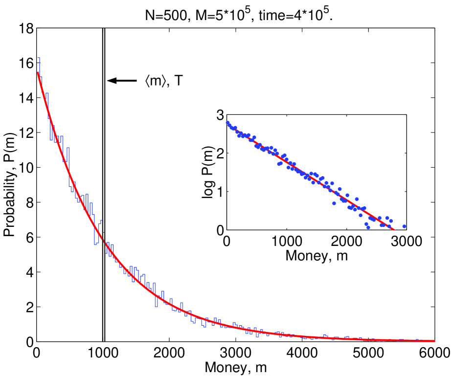
FIG. 1.: Histogram and points: stationary probability distribution of money $P(m)$. Solid curves: fits to the Boltzmann-Gibbs law $P(m)\propto\exp(-m/T)$. Vertical lines: the initial distribution of money.

To check that these general arguments indeed work, we performed several computer simulations. Initially, all agents are given the same amount of money: $P(m)=\delta(m-M/N)$, which is shown in Fig. 1 as the double vertical line. One pair of agents at a time is chosen randomly, then one of the agents is randomly picked to be the “winner” (the other agent becomes the “loser”), and the amount $\Delta m\geq 0$ is transferred from the loser to the winner. If the loser does not have enough money to pay ($m_{i}<\Delta m$), then the transaction does not take place, and we proceed to another pair of agents. Thus, the agents are not permitted to have negative money. This boundary condition is crucial in establishing the stationary distribution. As the agents exchange money, the initial delta-function distribution first spread symmetrically. Then, the probability density starts to pile up at the impenetrable boundary $m=0$. The distribution becomes asymmetric (skewed) and ultimately reaches the stationary exponential shape shown in Fig. 1. We used several trading rules in the simulations: the exchange of a small constant amount $\Delta m=1$, the exchange of a random fraction $0\leq\nu\leq 1$ of the average money of the pair: $\Delta m=\nu(m_{i}+m_{j})/2$, and the exchange of a random fraction $\nu$ of the average money in the system: $\Delta m=\nu\,M/N$. Figures in the paper mostly show simulations for the third rule; however, the final stationary distribution was found to be the same for all rules.

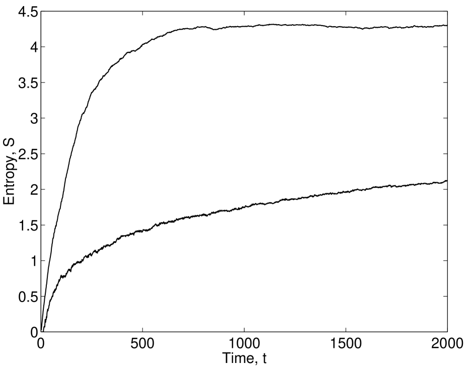
FIG. 2.: Time evolution of entropy. Top curve: for the exchange of a random fraction $\nu$ of the average money in the system: $\Delta m=\nu\,M/N$. Bottom curve: for the exchange of a small constant amount $\Delta m=1$. The time scale for the bottom curve is 500 times greater than indicated, so it actually ends at the time $10^{6}$.

In the process of evolution, the entropy $S$ increases in time and saturates at the maximal value for the Boltzmann-Gibbs distribution. This is illustrated by the top curve in Fig. 2 computed for the third rule of exchange. The bottom curve in Fig. 2 shows the time evolution of entropy for the first rule of exchange. The time scale for this curve is 500 times greater than for the top curve, so the bottom curve actually ends at the time $10^{6}$. The plot shows that, for the first rule of exchange, mixing is much slower than for the third one. Nevertheless, even for the first rule, the system also eventually reaches the Boltzmann-Gibbs state of maximal entropy, albeit over a time much longer than shown in Fig. 2.

One might argue that the pairwise exchange of money may correspond to a medieval market, but not to a modern economy. In order to make the model somewhat more realistic, we introduce firms. One agent at a time becomes a “firm”. The firm borrows capital $K$ from another agent and returns it with an interest $rK$, hires $L$ agents and pays them wages $W$, manufactures $Q$ items of a product and sell it to $Q$ agents at a price $R$. All of these agents are randomly selected. The firm receives the profit $F=RQ-LW-rK$. The net result is a many-body exchange of money that still satisfies the conservation law.

Parameters of the model are selected following the procedure described in economics textbooks. The aggregate demand-supply curve for the product is taken to be $R(Q)=V/Q^{\eta}$, where $Q$ is the quantity people would buy at a price $R$, and $\eta=0.5$ and $V=100$ are constants. The production function of the firm has the conventional Cobb-Douglas form: $Q(L,K)=L^{\beta}K^{1-\beta}$, where $\beta=0.8$ is a constant. In our simulation, we set $W=10$. By maximizing firm’s profit $F$ with respect to $K$ and $L$, we find the values of the other parameters: $L=20$, $Q=10$, $R=32$, and $F=68$.

However, the actual values of the parameters do not matter. Our computer simulations show that the stationary probability distribution of money in this model always has the universal Boltzmann-Gibbs form independent of the model parameters.

IV Thermal machine

As explained in Introduction, the money distribution $P(m)$ should not be confused with the distribution of wealth. We believe that $P(m)$ should be interpreted as the instantaneous distribution of purchasing power in the system. Indeed, to make a purchase, one needs money. Material wealth normally is not used directly for a purchase. It needs to be sold first to be converted into money.

Let us consider an outside monopolistic vendor selling a product (say, cars) to the system of agents at a price $p$. Suppose that a certain small fraction $f$ of the agents needs to buy the product at a given time, and each agent who has enough money to afford the price will buy one item. The fraction $f$ is assumed to be sufficiently small, so that the purchase does not perturb the whole system significantly. At the same time, the absolute number of agents in this group is assumed to be big enough to make the group statistically representative and characterized by the Boltzmann-Gibbs distribution of money. The agents in this group continue to exchange money with the rest of the system, which acts as a thermal bath. The demand for the product is constantly renewed, because products purchased in the past expire after a certain time. In this situation, the vendor can sell the product persistently, thus creating a small steady leakage of money from the system to the vendor.

What price $p$ would maximize the vendor’s income? To answer this question, it is convenient to introduce the cumulative distribution of purchasing power ${\cal N}(m)=N\int_{m}^{\infty}P(m^{\prime})\,dm^{\prime}=Ne^{-m/T}$, which gives the number of agents whose money is greater than $m$. The vendor’s income is $fp{\cal N}(p)$. It is maximal when $p=T$, i. e. the optimal price is equal to the temperature of the system. This conclusion also follows from the simple dimensional argument that temperature is the only money scale in the problem. At the price $p=T$ that maximizes the vendor’s income, only the fraction ${\cal N}(T)/N=e^{-1}=0.37$ of the agents can afford to buy the product.

Now let us consider two disconnected economic systems, one with the temperature $T_{1}$ and another with $T_{2}$: $T_{1}>T_{2}$. A vendor can buy a product in the latter system at its equilibrium price $T_{2}$ and sell it in the former system at the price $T_{1}$, thus extracting the speculative profit $T_{1}-T_{2}$, as in a thermal machine. This example suggests that speculative profit is possible only when the system as a whole is out of equilibrium. As money is transferred from the high- to the low-temperature system, their temperatures become closer and eventually equal. After that, no speculative profit is possible, which would correspond to the “thermal death” of the economy. This example brings to mind economic relations between developed and developing countries, with manufacturing in the poor (low-temperature) countries for export to the rich (high-temperature) ones.

V Models with debt

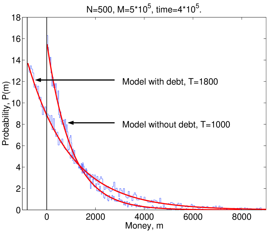
FIG. 3.: Histograms: stationary distributions of money with and without debt. Solid curves: fits to the Boltzmann-Gibbs laws with temperatures $T=1800$ and $T=1000$.

Now let us discuss what happens if the agents are permitted to go into debt. Debt can be viewed as negative money. Now when a loser does not have enough money to pay, he can borrow the required amount from a reservoir, and his balance becomes negative. The conservation law is not violated: The sum of the winner’s positive money and loser’s negative money remains constant. When an agent with a negative balance receives money as a winner, she uses this money to repay the debt until her balance becomes positive. We assume for simplicity that the reservoir charges no interest for the lent money. However, because it is not sensible to permit unlimited debt, we put a limit $m_{d}$ on the maximal debt of an agent: $m_{i}>-m_{d}$. This new boundary condition $P(m<-m_{d})=0$ replaces the old boundary condition $P(m<0)=0$. The result of a computer simulation with $m_{d}=800$ is shown in Fig. 3 together with the curve for $m_{d}=0$. $P(m)$ is again given by the Boltzmann-Gibbs law, but now with the higher temperature $T=M/N+m_{d}$, because the normalization conditions need to be maintained including the population with negative money: $\int_{-m_{d}}^{\infty}P(m)\,dm=1$ and $\int_{-m_{d}}^{\infty}m\,P(m)\,dm=M/N$. The higher temperature makes the money distribution broader, which means that debt increases inequality between agents [10].

Imposing a sharp cutoff at $m_{d}$ may be not quite realistic. In practice, the cutoff may be extended over some range depending on the exact bankruptcy rules. Over this range, the Boltzmann-Gibbs distribution would be smeared out. So we expect to see the Boltzmann-Gibbs law only sufficiently far from the cutoff region. Similarly, in experiment [5], some deviations from the exponential law were observed near the lower boundary of the distribution. Also, at the high end of the distributions, the number of events becomes small and statistics poor, so the Boltzmann-Gibbs law loses applicability. Thus, we expect the Boltzmann-Gibbs law to hold only for the intermediate range of money not too close either to the lower boundary or to the very high end. However, this range is the most relevant, because it covers the great majority of population.

Lending creates equal amounts of positive (asset) and negative (liability) money [6, 8]. When economics textbooks describe how “banks create money” or “debt creates money” [8], they do not count the negative liabilities as money, and thus their money is not conserved. In our operational definition of money, we include all financial instruments with fixed denomination, such as currency, IOUs, and bonds, but not material wealth or stocks, and we count both assets and liabilities. With this definition, money is conserved, and we expect to see the Boltzmann-Gibbs distribution in equilibrium. Unfortunately, because this definition differs from economists’ definitions of money (M1, M2, M3, etc. [8]), it is not easy to find the appropriate statistics. Of course, money can be also emitted by a central bank or government. This is analogous to an external influx of energy into a physical system. However, if this process is sufficiently slow, the economic system may be able to maintain quasi-equilibrium, characterized by a slowly changing temperature.

We performed a simulation of a model with one bank and many agents. The agents keep their money in accounts on which the bank pays interest. The agents may borrow money from the bank, for which they must pay interest in monthly installments. If they cannot make the required payments, they may be declared bankrupt, which relieves them from the debt, but the liability is transferred to the bank. In this way, the conservation of money is maintained. The model is too elaborate to describe it in full detail here. We found that, depending on the parameters of the model, either the agents constantly lose money to the bank, which steadily reduces the agents’ temperature, or the bank constantly loses money, which drives down its own negative balance and steadily increases the agents’ temperature.

VI Boltzmann equation

The Boltzmann-Gibbs distribution can be also derived from the Boltzmann equation [11], which describes the time evolution of the distribution function $P(m)$ due to pairwise interactions:

$$\frac{dP(m)}{dt}=\int\!\int\{-w_{[m,m^{\prime}]\to[m-\Delta,m^{\prime}+\Delta]}P(m)P(m^{\prime})$$ (1)

$$+w_{[m-\Delta,m^{\prime}+\Delta]\to[m,m^{\prime}]}P(m-\Delta)P(m^{\prime}+\Delta)\}\,dm^{\prime}\,d\Delta.$$ (2)

Here $w_{[m,m^{\prime}]\to[m-\Delta,m^{\prime}+\Delta]}$ is the rate of transferring money $\Delta$ from an agent with money $m$ to an agent with money $m^{\prime}$. If a model has time-reversal symmetry, then the transition rate of a direct process is the same as the transition rate of the reversed process, thus the $w$-factors in the first and second lines of Eq. (1) are equal. In this case, the Boltzmann-Gibbs distribution $P(m)=C\exp(-m/T)$ nullifies the right-hand side of Eq. (1); thus this distribution is stationary: $dP(m)/dt=0$ [11].

VII Non-Boltzmann-Gibbs distributions

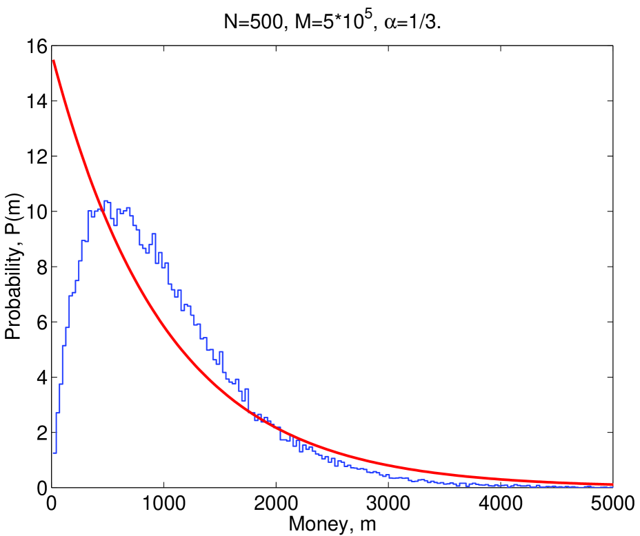
FIG. 4.: Histogram: stationary probability distribution of money in the multiplicative random exchange model studied in Ref. [7]. Solid curve: the Boltzmann-Gibbs law.

However, if time-reversal symmetry is broken, the two transition rates $w$ in Eq. (1) may be different, and the system may have a non-Boltzmann-Gibbs stationary distribution or no stationary distribution at all. Examples of such kind were studied in Ref. [7]. One model was called the multiplicative random exchange. In this model, a randomly selected loser $i$ loses a fixed fraction $\alpha$ of his money $m_{i}$ to a randomly selected winner $j$: $[m_{i},m_{j}]\to[(1-\alpha)m_{i}\>,\>m_{j}+\alpha m_{i}]$. If we try to reverse this process and appoint the winner $j$ to become a loser, the system does not return to the original configuration $[m_{i},m_{j}]$: $[(1-\alpha)m_{i}\>,\>m_{j}+\alpha m_{i}]\to[(1-\alpha)m_{i}+\alpha(m_{j}+\alpha m_{i})\>,\>(1-\alpha)(m_{j}+\alpha m_{i})]$. Except for $\alpha=1/2$, the exponential distribution function is not a stationary solution of the Boltzmann equation derived for this model in Ref. [7]. Instead, the stationary distribution has the shape shown in Fig. 4 for $\alpha=1/3$, which we reproduced in our numerical simulations. It still has an exponential tail end at the high end, but drops to zero at the low end for $\alpha<1/2$. Another example of similar kind was studied in Ref. [12], which appeared after the first version of our paper was posted as cond-mat/0001432 on January 30, 2000. In that model, the agents save a fraction $\lambda$ of their money and exchange a random fraction $\epsilon$ of their total remaining money: $[m_{i},m_{j}]\to[\lambda m_{i}+\epsilon(1-\lambda)(m_{i}+m_{j})\>,\>\lambda m_{j}+(1-\epsilon)(1-\lambda)(m_{i}+m_{j})]$. This exchange also does not return to the original configuration after being reversed. The stationary probability distribution was found in Ref. [12] to be nonexponential for $\lambda\neq 0$ with a shape qualitatively similar to the one shown in Fig. 4.

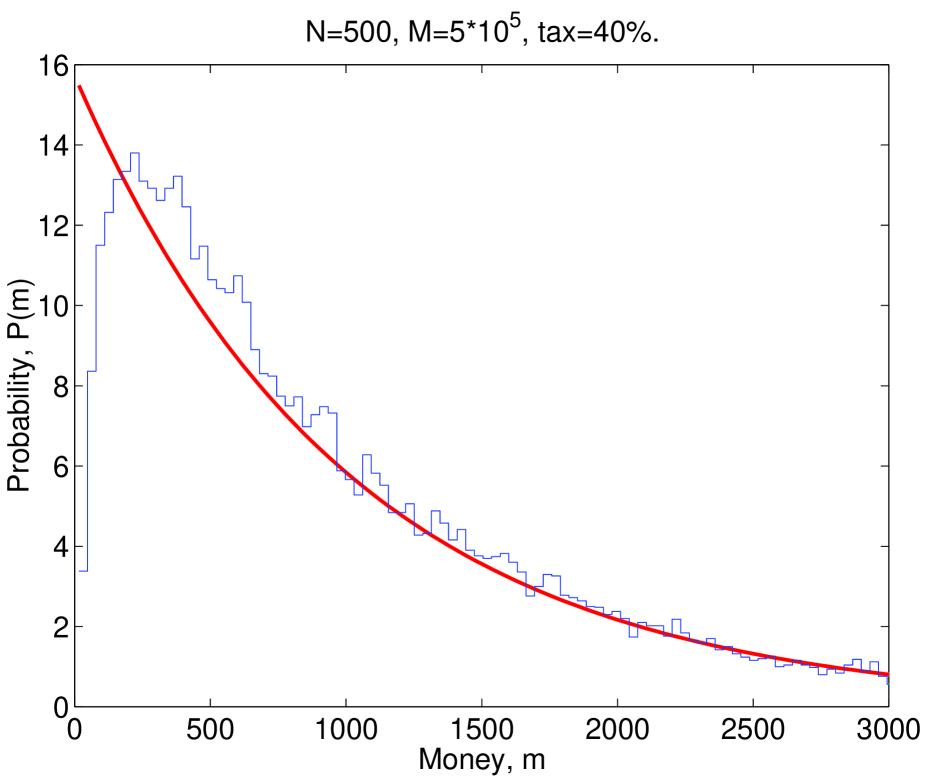
FIG. 5.: Histogram: stationary probability distribution of money in the model with taxes and subsidies. Solid curve: the Boltzmann-Gibbs law.

Another interesting example of a non-Boltzmann-Gibbs distribution occurs in a model with taxes and subsidies. Suppose a special agent (“government”) collects a fraction (“tax”) of every transaction in the system. The collected money is then equally divided between all agents of the system, so that each agent receives the subsidy $\delta m$ with the frequency $1/\tau_{s}$. Assuming that $\delta m$ is small and approximating the collision integral with a relaxation time $\tau_{r}$ [11], we obtain the following Boltzmann equation

$$\frac{\partial P(m)}{\partial t}+\frac{\delta m}{\tau_{s}}\,\frac{\partial P(m)}{\partial m}=-\frac{P(m)-\tilde{P}(m)}{\tau_{r}},$$ (3)

where $\tilde{P}(m)$ is the equilibrium Boltzmann-Gibbs function. The second term in the left-hand side of Eq. (3) is analogous to the force applied to electrons in a metal by an external electric field [11]. The approximate stationary solution of Eq. (3) is the displaced Boltzmann-Gibbs one: $P(m)=\tilde{P}(m-(\tau_{r}/\tau_{s})\,\delta m)$. The displacement of the equilibrium distribution $\tilde{P}(m)$ by $(\tau_{r}/\tau_{s})\,\delta m$ would leave an empty gap near $m=0$. This gap is filled by interpolating between zero population at $m=0$ and the displaced distribution. The curve obtained in a computer simulation of this model (Fig. 5) qualitatively agrees with this expectation. The low-money population is suppressed, because the government, acting as an external force, “pumps out” that population and pushes the system out of thermodynamic equilibrium. We found that the entropy of the stationary state in the model with taxes and subsidies is few percents lower than without.

These examples show that the Boltzmann-Gibbs distribution is not fully universal, meaning that it does not hold for just any model of exchange that conserves money. Nevertheless, it is universal in a limited sense: For a broad class of models that have time-reversal symmetry, the stationary distribution is exponential and does not depend on the details of a model. Conversely, when time-reversal symmetry is broken, the distribution may depend on model details. The difference between these two classes of models may be rather subtle. For example, let us change the multiplicative random exchange from a fixed fraction of loser’s money to a fixed fraction of the total money of winner and loser. This modification retains the multiplicative idea that the amount exchanged is proportional to the amount involved, but restores time-reversal symmetry and the Boltzmann-Gibbs distribution. In the model with $\Delta m=1$ discussed in the next Section, the difference between time-reversible and time-irreversible formulations amounts to the difference between impenetrable and absorbing boundary conditions at $m=0$. Unlike in physics, in economy there is no fundamental requirement that interactions have time-reversal symmetry. However, in the absence of detailed knowledge of real microscopic dynamics of economic exchange, the semiuniversal Boltzmann-Gibbs distribution appears to be a natural starting point.

Moreover, deviations from the Boltzmann-Gibbs law may occur only if the transition rates $w$ in Eq. (1) explicitly depend on the agents money $m$ or $m^{\prime}$ in an asymmetric manner. In another simulation, we randomly preselected winners and losers for every pair of agents $(i,j)$. In this case, money flows along directed links between the agents: $i\!\to\!j\!\to\!k$, and time-reversal symmetry is strongly broken. This model is closer to the real economy, in which, for example, one typically receives money from an employer and pays it to a grocer, but rarely the reverse. Nevertheless, we still found the Boltzmann-Gibbs distribution of money in this model, because the transition rates $w$ do not explicitly depend on $m$ and $m^{\prime}$.

VIII Nonlinear Boltzmann equation vs. linear master equation

For the model where agents randomly exchange the constant amount $\Delta m=1$, the Boltzmann equation is:

$$\frac{dP_{m}}{dt} = P_{m+1}\sum\limits_{n=0}^{\infty}P_{n}+P_{m-1}\sum\limits_{n=1}^{\infty}P_{n}$$ (5)

$${}-P_{m}\sum\limits_{n=0}^{\infty}P_{n}-P_{m}\sum\limits_{n=1}^{\infty}P_{n}$$

$$= (P_{m+1}+P_{m-1}-2P_{m})+P_{0}(P_{m}-P_{m-1}),$$ (6)

where $P_{m}\equiv P(m)$ and we have used $\sum_{m=0}^{\infty}P_{m}=1$. The first, diffusion term in Eq. (6) is responsible for broadening of the initial delta-function distribution. The second term, proportional to $P_{0}$, is essential for the Boltzmann-Gibbs distribution $P_{m}=e^{-m/T}(1-e^{-1/T})$ to be a stationary solution of Eq. (6). In a similar model studied in Ref. [7], the second term was omitted on the assumption that agents who lost all money are eliminated: $P_{0}=0$. In that case, the total number of agents is not conserved, and the system never reaches any stationary distribution. Time-reversal symmetry is violated, since transitions into the state $m=0$ are permitted, but not out of this state.

If we treat $P_{0}$ as a constant, Eq. (6) looks like a linear Fokker-Planck equation [11] for $P_{m}$, with the first term describing diffusion and the second term an external force proportional to $P_{0}$. Similar equations were studied in Ref. [9]. Eq. (6) can be also rewritten as

$$\frac{dP_{m}}{dt}=P_{m+1}-(2-P_{0})P_{m}+(1-P_{0})P_{m-1}.$$ (7)

The coefficient $(1-P_{0})$ in front of $P_{m-1}$ represents the rate of increasing money by $\Delta m=1$, and the coefficient 1 in front of $P_{m+1}$ represents the rate of decreasing money by $\Delta m=-1$. Since $P_{0}>0$, the former is smaller than the latter, which results in the stationary Boltzmann-Gibbs distributions $P_{m}=(1-P_{0})^{m}$. An equation similar to Eq. (7) describes a Markov chain studied for strategic market games in Ref. [13]. Naturally, the stationary probability distribution of wealth in that model was found to be exponential [13].

Even though Eqs. (6) and (7) look like linear equations, nevertheless the Boltzmann equation (1) and (5) is a profoundly nonlinear equation. It contains the product of two probability distribution functions $P$ in the right-hand side, because two agents are involved in money exchange. Most studies of wealth distribution [9] have the fundamental flaw that they use a single-particle approach. They assume that the wealth of an agent may change just by itself and write a linear master equation for the probability distribution. Because only one particle is considered, this approach cannot adequately incorporate conservation of money. In reality, an agent can change money only by interacting with another agent, thus the problem requires a two-particle probability distribution function. Using Boltzmann’s molecular chaos hypothesis, the two-particle function is factorized into a product of two single-particle distributions functions, which results in the nonlinear Boltzmann equation. Conservation of money is adequately incorporated in this two-particle approach, and the universality of the exponential Boltzmann-Gibbs distribution is transparent.

IX Conclusions

Everywhere in the paper we assumed some randomness in the exchange of money. The results of our paper would apply the best to the probability distribution of money in a closed community of gamblers. In more traditional economic studies, the agents exchange money not randomly, but following deterministic strategies, such as maximization of utility functions [6, 14]. The concept of equilibrium in these studies is similar to mechanical equilibrium in physics, which is achieved by minimizing energy or maximizing utility. However, for big ensembles, statistical equilibrium is a more relevant concept. When many heterogeneous agents deterministically interact and spend various amounts of money from very little to very big, the money exchange is effectively random. In the future, we would like to uncover the Boltzmann-Gibbs distribution of money in a simulation of a big ensemble of economic agents following realistic deterministic strategies with money conservation taken into account. That would be the economics analog of molecular dynamics simulations in physics. While atoms collide following fully deterministic equations of motion, their energy exchange is effectively random due to complexity of the system and results in the Boltzmann-Gibbs law.

We do not claim that the real economy is in equilibrium. (Most of the physical world around us is not in true equilibrium either.) Nevertheless, the concept of statistical equilibrium is a very useful reference point for studying nonequilibrium phenomena.

The authors are grateful to M. Gubrud for helpful discussion and proofreading of an earlier version of the manuscript.

Note added: After the paper had been submitted for publication, we have learned about the book by Aoki [15], who applied many ideas of statistical physics to economics, albeit not specifically to the distribution of money.

REFERENCES

-
[1]
E-mail: yakovenk@physics.umd.edu
Web: http://www2.physics.umd.edu/~yakovenk - [2] J. D. Farmer, Computing in Science and Engineering 1, #6, p. 26 (1999); R. N. Mantegna and H. E. Stanley, An Introduction to Econophysics (Cambridge University Press, Cambridge, 2000).
- [3] G. H. Wannier, Statistical Physics (Dover, New York, 1987).
- [4] It is also implied that the system is extensive. We study only extensive models, so the nonextensive generalization of entropy by C. Tsallis, J. Stat. Phys. 52, 479 (1988); Braz. J. Phys. 29, 1 (1999) is not relevant for our consideration.
- [5] D. M. Mueth, H. M. Jaeger, and S. R. Nagel, Phys. Rev. E 57, 3164 (1998); M. L. Nguyen and S. N. Coppersmith, Phys. Rev. E 59, 5870 (1999).
- [6] M. Shubik, in The Economy as an Evolving Complex System II, edited by W. B. Arthur, S. N. Durlauf, and D. A. Lane (Addison-Wesley, Reading, 1997) p. 263.
- [7] S. Ispolatov, P. L. Krapivsky, and S. Redner, Eur. Phys. J. B 2, 267 (1998).
- [8] C. R. McConnell and S. L. Brue, Economics: Principles, Problems, and Policies (McGraw-Hill, New York, 1996).
- [9] E. W. Montroll and M. F. Shlesinger, Proc. Natl. Acad. Sci. USA 79, 3380 (1982); O. Malcai, O. Biham, and S. Solomon, Phys. Rev. E 60, 1299 (1999); D. Sornette and R. Cont, J. Phys. I (France) 7, 431 (1997); J.-P. Bouchaud and M. Mézard, cond-mat/0002374.
-
[10]
In general, temperature is completely determined by the
average money per agent, , and the boundary
conditions. Suppose the agents are required to have no less money
than and no more than : . In this
case, the normalization conditions and
with
give the following equation for :
where and . It follows from Eq. (8) that the temperature is positive when , negative when , and infinite () when . In particular, if agents’ money are bounded from above, but not from below: , the temperature is negative. That means inverted Boltzmann-Gibbs distribution with more reach agents than poor.(8) - [11] E. M. Lifshitz and L. P. Pitaevskiĭ, Physical Kinetics (Pergamon Press, New York, 1993).
- [12] A. Chakraborti and B. K. Chakrabarty, cond-mat/0004256, to be published in Eur. Phys. J. B.
- [13] Martin Shubik, The Theory of Money and Financial Institutions, vol. 2 (The MIT Press, Cambridge, 1999), p. 192.
- [14] P. Bak, S. F. Nørrelykke, and M. Shubik, Phys. Rev. E 60, 2528 (1999).
- [15] Masanao Aoki, New Approaches to Macroeconomic Modeling (Cambridge University Press, Cambridge, 1996).