Statistics and noise in a quantum measurement process

Abstract

The quantum measurement process by a single-electron transistor or a quantum point contact coupled to a quantum bit is studied. We find a unified description of the statistics of the monitored quantity, the current, in the regime of strong measurement and expect this description to apply for a wide class of quantum measurements. We derive the probability distributions for the current and charge in different stages of the process. In the parameter regime of the strong measurement the current develops a telegraph-noise behavior which can be detected in the noise spectrum.

Introduction.

The long-standing interest in fundamental questions of the quantum measurement received new impetus by the experimental progress in mesoscopic physics and increasing activities in quantum state engineering. The basic idea is to use as meter a device, able to carry a macroscopic current, which is coupled to the quantum system such that the conductance depends on the quantum state. By monitoring the current one performs a quantum measurement, which, in turn, causes a dephasing of the quantum system [1, 2, 3]. The dephasing has been demonstrated in an experiment of Buks et al. [4] where a quantum dot is embedded in one arm of a ‘which-path’ interferometer. The current through a quantum point contact (QPC) in close proximity to the dot suppresses the interference. However, since passing electrons interact with the current only for a short dwell-time in the dot, the meter fails to distinguish between two possible paths of individual electron; only a reduction of interference has been observed. This situation is referred to as a weak measurement.

For a strong quantum measurement a different setting is needed, where a closed quantum system is observed by a meter. Then a sufficiently long observation may provide information about the quantum state. This situation is realized when a single-electron transistor (SET) is coupled to a Josephson junction single-charge box, which for suitable parameters serves as a quantum bit (qubit) [5, 6]. The analysis of the time evolution of the density matrix of the coupled system demonstrates the mutual influence between qubit and meter, i.e. measurement and dephasing [7].

The measurement process is characterized by three time scales. On the shortest, the dephasing time $\tau_{\varphi}$, the phase coherence between two eigenstates of the qubit is lost, while their occupation probabilities remain unchanged. Later measurement-induced transitions mix the eigenstates, changing their occupation probabilities on a time scale $t_{\rm mix}>\tau_{\varphi}$ and erasing information about the initial state of the qubit. The origin of the mixing is that the charge operator (the measured quantity) and the qubit’s Hamiltonian do not commute. The third time scale appears in the dynamics of the current in the SET. Consider the probability distribution $P(m,t)$ that $m$ electrons have tunneled through the SET by time $t$. It was shown [7] that after a certain time $t_{\rm meas}$ information about the state of the qubit can be extracted by reading out $m$. As expected from the basic principles of quantum mechanics the observation of the qubit first of all disturbs its state. Hence $t_{\rm meas}\geq\tau_{\varphi}$. The measurement process is only effective if the mixing is slow, $t_{\rm mix}\gg t_{\rm meas}$. In the opposite limit of strong mixing the information about the qubit’s state is lost before a read-out is achieved.

The distribution function $P(m,t)$ describes the statistics of the charge which has tunneled. The distribution of the current in the SET $p(I,t)$ and current-current correlations require, furthermore, the knowledge of correlations of the values of $m$ at different times. In earlier papers on the statistics in a SET [7] or a QPC [8, 9] the behavior of $P(m,t)$ at times shorter than $t_{\rm mix}$ was derived. Effects due to the additional knowledge acquired by an observer [10], and the possible influence of the wave-function collapse on the monitored current [8] were also discussed. Here we develop a systematic approach, based on the time evolution (Schrödinger equation) of the density matrix of the coupled system. This approach allows us to study averages and correlators of the current and charge. Since, due to shot noise, instantaneous values of the current fluctuate strongly, we study the current ${\bar{I}}$, averaged over a finite time interval $\Delta t$. We calculate the mixing time in a SET and derive analytic expressions for $p({\bar{I}},{\Delta t},t)$, as well as $P(m,t)$, valid on both short and long time scales. We study the noise spectrum of the current and find that in the limit of strong measurement ($t_{\rm meas}<t_{\rm mix}$) the long-time dynamics is characterized by telegraph noise, with jumps between two possible current values, corresponding to two qubit’s eigenstates.

The results are of immediate experimental interest. A recent experiment demonstrated the quantum coherence in a macroscopic superconducting electron box [11], but the coherence time was limited by the measuring device. The SET-based measurement should extend the coherence time, which combined with experimental progress in fast measurement techniques [12] should increase the maximum number of coherent quantum manipulations.

Master equation for the measurement by a SET. The system of a qubit coupled to a SET is shown in Fig. 1. The qubit is a Josephson junction in the Coulomb blockade regime. Its dynamics is limited to a two-dimensional Hilbert space spanned by two charge states, with $n=0$ or $1$ extra Cooper pair on a superconducting island. The island is coupled capacitively to the middle island of the SET, influencing the transport current. The SET is kept in the off-state during manipulations on the qubit [7], with no dissipative current and no additional decoherence. To perform the measurement, the transport voltage is switched to a sufficiently high value, so that the current starts to flow in the SET.

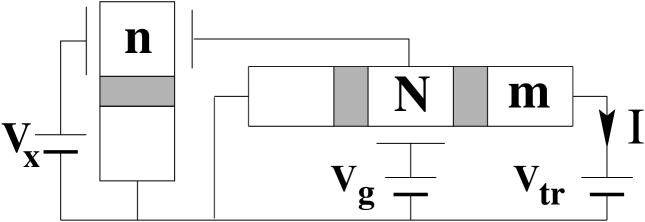
FIG. 1.: The circuit of a qubit and a SET used as a meter.

The Hamiltonian of the system is given by [13]

$${\cal H}={\cal H}_{\rm SET}+{\cal H}_{\rm qb}^{N}+{\cal H}_{\rm T}+{\cal H}_{\rm\psi}\;.$$ (1)

The first term is the charging energy of the transistor, quadratic in the charge $Ne$ on the middle island, ${\cal H}_{\rm SET}=E_{\rm SET}(N-N_{0})^{2}$. The induced charge $N_{0}e$ is determined by the gate voltage $V_{\rm g}$ and other voltages in the circuit. The Hamiltonian of the qubit, ${\cal H}_{\rm qb}^{N}={\cal H}_{\rm qb}+N{\cal H}_{\rm int}$, includes the Hamiltonian of the uncoupled qubit ${\cal H}_{\rm qb}$ and the Coulomb interaction with the SET $N{\cal H}_{\rm int}$ (split into two terms for later convenience.) In the basis of the qubit’s charge states they are given by ${\cal H}_{\rm qb}=\frac{1}{2}(E_{\rm qb}\hat{\sigma}_{z}-E_{\rm J}\hat{\sigma}_{x})$ and $N{\cal H}_{\rm int}=E_{\rm int}N\hat{\sigma}_{z}$. The charging energy scales $E_{\rm SET}$, $E_{\rm qb}$ and $E_{\rm int}$ are determined by capacitances in the circuit, while $E_{\rm J}$ is the Josephson coupling. We consider the eigenstates of ${\cal H}_{\rm qb}$, $|0\rangle$ and $|1\rangle$, as the logical states of the qubit. In this basis, ${\cal H}_{\rm qb}$ is diagonal, with the level spacing $\Delta E\equiv(E_{\rm J}^{2}+E_{\rm qb}^{2})^{1/2}$, while ${\cal H}_{\rm int}=\left(\begin{array}[]{cc}E_{\rm int}^{\parallel}&E_{\rm int}^{\perp}\\ E_{\rm int}^{\perp}&-E_{\rm int}^{\parallel}\end{array}\right)$, where $E_{\rm int}^{\parallel}\equiv E_{\rm int}E_{\rm qb}/\Delta E$ and $E_{\rm int}^{\perp}\equiv E_{\rm int}E_{\rm J}/\Delta E$. The term ${\cal H}_{\rm\psi}$ describes the Fermions in the island and electrodes of the SET, while ${\cal H}_{\rm T}$ governs the tunneling in the SET. Here we assume weak coupling to the environment, with relaxation slower than the SET-induced mixing. The opposite limit is dicussed in Ref. [13].

The full density matrix can be reduced to $\rho^{iN\phantom{{}^{\prime}}m\phantom{{}^{\prime}}}_{jN^{\prime}m^{\prime}}(t)$ by tracing over microscopic degrees of freedom and keeping track only of $N$ and $m$, the number of electrons which have tunneled through the SET. Here $i,j=0,1$ refer to a qubit’s basis. A closed set of equations can be derived for $\rho_{N}^{ij}(m)\equiv\rho^{iNm}_{jNm}$, the diagonal entries of the density matrix in $N$ and $m$ [14]. Solving these equations, we analyze the evolution of the reduced density matrix of the qubit, $\varrho^{ij}(t)\equiv\sum_{N,m}\rho_{N}^{ij}(m,t)$, as well as $P(m,t)\equiv\sum_{N,j}\rho_{N}^{jj}(m,t)$ and other statistical characteristics of the current in the SET.

At low temperatures and transport voltages only two charge states of the middle island of the SET, with $N$ and $N+1$ electrons, contribute to the dynamics. Translational invariance in $m$-space suggests the Fourier transformation $\rho_{N}^{ij}(k)\equiv\sum_{m}e^{-{\rm i}km}\rho_{N}^{ij}(m)$. Expanding in the tunneling term to lowest order, we obtain the following master equation (cf. Refs. [7, 13]):

$$\hbar\frac{d}{dt}\left(\begin{array}[]{c}\hat{\rho}_{N\phantom{+1}}\\ \hat{\rho}_{N+1}\end{array}\right) + \left(\begin{array}[]{c}{\rm i}\,[{\cal H}_{\rm qb},\hat{\rho}_{N}]\\[3.0pt] {\rm i}\,[{\cal H}_{\rm qb}+{\cal H}_{\rm int},\hat{\rho}_{N+1}]\end{array}\right)$$ (6)

$$= \left(\begin{array}[]{cc}-\check{\Gamma}_{L}&e^{{\rm i}k}\check{\Gamma}_{R}\\ \phantom{-}\check{\Gamma}_{L}&-\check{\Gamma}_{R}\end{array}\right)\left(\begin{array}[]{c}\hat{\rho}_{N\phantom{+1}}\\ \hat{\rho}_{N+1}\end{array}\right)\;.$$ (11)

Here the operators

$$\check{\Gamma}_{L}\hat{\rho} \equiv \Gamma_{L}\hat{\rho}+\pi\alpha_{L}\;[{\cal H}_{\rm int},\hat{\rho}]_{+}\;,$$ (12)

$$\check{\Gamma}_{R}\hat{\rho} \equiv \Gamma_{R}\hat{\rho}-\pi\alpha_{R}\;[{\cal H}_{\rm int},\hat{\rho}]_{+}\;.$$ (13)

represent the tunneling rates in the left and right junctions, with $\alpha_{\rm L/R}\equiv R_{\rm K}/(8\pi^{3}R^{\rm T}_{\rm L/R})$ being the tunnel conductance of the junctions in units of the resistance quantum $R_{\rm K}=h/e^{2}$. The rates are fixed by the potentials $\mu_{L}$, $\mu_{R}=\mu_{L}+V_{\rm tr}$ of the leads: $\Gamma_{L}=2\pi\alpha_{L}[\mu_{L}-(1-2N_{0})E_{\rm SET}]$ and $\Gamma_{R}=2\pi\alpha_{R}[(1-2N_{0})E_{\rm SET}-\mu_{R}]$. They define the tunneling rate $\Gamma=\Gamma_{L}\Gamma_{R}/(\Gamma_{L}+\Gamma_{R})$ through the SET. The last terms in Eqs. (12,13) make these rates sensitive to the qubit’s state.

The initial condition at the beginning of the measurement, written down in the logical basis,

$$\rho^{ij}_{N}(m,t=0)=\left(\begin{array}[]{cc}|a|^{2}&ab^{*}\\ a^{*}b&|b|^{2}\end{array}\right)w_{N}\;\delta_{m0}\ ,$$ (14)

describes the qubit in a pure state $a|0\rangle+b|1\rangle$ and the SET in the zero-voltage equilibrium state. One can assume that $w_{N}=1$ and $w_{N+1}=0$.

Reduction of the master equation.

In general the dynamics of the qubit’s density matrix $\hat{\varrho}$, described by the master equation (11), is complicated since dephasing (decay of the off-diagonal entries) and mixing (relaxation of the diagonal to their stationary values) may occur on similar time scales, $\tau_{\varphi}\approx t_{\rm mix}$. However, under suitable conditions the mixing is slow, which is the prerequisite for a measurement process. This is the case, if the qubit operates in the regime with dominant charging energy:

$$|E_{\rm qb}|,|E_{\rm qb}+2E_{\rm int}|\gg E_{\rm J}\ .$$ (15)

Weak ($E_{\rm int}\ll\Delta E$) or strong ($E_{\rm int}\!\sim\!\Delta E$) coupling to the SET can be considered. In the latter case a faster measurement is achieved (see Eq. (29)).

We first analyze the dynamics without mixing, i.e. we put $E_{\rm int}^{\perp}=0$. In this case the time evolutions of $\rho_{N}^{ij}$ for the four different pairs of indices $ij$ are decoupled from each other, each being characterized by two eigenmodes. The absence of mixing, further, implies the conservation of occupations of the logical states $\varrho^{ii}$, for $i=0,1$, and we find two ‘Goldstone’ modes for $k\ll 1$, with eigenvalues

$$\lambda^{ii}_{+}(k)\approx{\rm i}\,\Gamma^{{i}}k-\frac{1}{2}f^{i}\Gamma^{{i}}k^{2}\ .$$ (16)

Here $\Gamma^{i}\equiv\Gamma_{L}^{i}\Gamma_{R}^{i}/(\Gamma_{L}^{i}+\Gamma_{R}^{i})$ are the tunneling rates through the SET, $\Gamma_{L}^{0/1}=\Gamma_{L}\pm\pi\alpha_{L}E_{\rm int}^{\parallel}$ and $\Gamma_{R}^{0/1}=\Gamma_{R}\mp\pi\alpha_{R}E_{\rm int}^{\parallel}$ are the tunneling rates in the junctions for two logical states (cf. Eqs. (12,13)), and $f^{i}\equiv 1-2\Gamma^{{i}}/(\Gamma_{L}^{i}+\Gamma_{R}^{i})$ are the Fano factors responsible for the shot noise reduction. The other two eigenmodes decay fast, with the rates $\lambda^{ii}_{-}\approx-(\Gamma^{{i}}_{L}+\Gamma^{{i}}_{R})$.

The analysis of the eigenvalues, $\lambda^{01}_{\pm}(k)=[\lambda^{10}_{\pm}(-k)]^{*}$, of the four off-diagonal modes in $ij$, reveals the dephasing time $\tau_{\varphi}$ of the qubit by the measurement, i.e., the decay time of $\varrho^{01}=\rho_{N}^{01}(k=0)+\rho_{N+1}^{01}(k=0)$. It is given by $\tau_{\varphi}^{-1}={4\Gamma E_{\rm int}^{\parallel\;2}}/{(\Gamma_{L}+\Gamma_{R})^{2}}$ if $E_{\rm int}^{\parallel}\ll\Gamma_{L}+\Gamma_{R}$, and $\tau_{\varphi}^{-1}=w_{N}\Gamma_{L}+w_{N+1}\Gamma_{R}$ in the opposite case.

The picture is modified by the mixing at finite $E_{\rm int}^{\perp}$. We find that the mixing may be treated perturbatively if $|\lambda^{01}_{\pm}|\gg E_{\rm int}^{\perp}$, which turns to be the case if the condition (15) holds. Then, in the second order, the degeneracy between the long-living modes (16) is lifted and the long-time evolution of the occupations $\rho^{ii}(k)=\rho^{ii}_{N}(k)+\rho^{ii}_{N+1}(k)$ is given by a reduced master equation,

$$\displaystyle\frac{d}{dt}\left(\begin{array}[]{cc}\rho^{00}(k)\\ \rho^{11}(k)\end{array}\right)=M_{\rm red}\left(\begin{array}[]{cc}\rho^{00}(k)\\ \rho^{11}(k)\end{array}\right)\;,$$ (21)

$$M_{\rm red}=\left(\begin{array}[]{cc}\lambda^{00}_{+}(k)&0\\ 0&\lambda^{11}_{+}(k)\end{array}\right)+\displaystyle\frac{1}{2}\Gamma_{\rm mix}\left(\begin{array}[]{cc}-1&\phantom{+}1\\ \phantom{+}1&-1\end{array}\right)\ .$$ (26)

For the mixing rate, $\Gamma_{\rm mix}$, we obtain

$$\Gamma_{\rm mix}\approx$$ (27)

$$\frac{4\Gamma E_{\rm J}^{2}E_{\rm int}^{2}}{\Delta E^{2}(\Delta E+2E_{\rm int}^{\parallel})^{2}+[\Gamma_{R}\Delta E+\Gamma_{L}(\Delta E+2E_{\rm int}^{\parallel})]^{2}}\;.$$ (28)

To understand the role of the mixing we assume first $\Gamma_{\rm mix}=0$ in Eqs. (21,26). Then, for the initial condition (14) we obtain $\rho^{00}(k)=|a|^{2}e^{\lambda_{+}^{00}(k)\;t}$, $\rho^{11}(k)=|b|^{2}e^{\lambda_{+}^{11}(k)\;t}$, and $P(k,t)\equiv\sum_{m}P(m,t)\,e^{-ikm}=\rho^{00}(k)+\rho^{11}(k)$. From this we obtain the distribution $P(m,t)$, which evolves from a peak $\delta(m)$ at $t=0$ into two peaks with weights $|a|^{2}$ and $|b|^{2}$, moving in $m$-space with velocities $\Gamma^{{0}}$ and $\Gamma^{{1}}$, and with widths growing as $\sqrt{2f^{i}\Gamma^{{i}}t}$. The peaks separate after a time

$$t_{\rm meas}=\left(\frac{\sqrt{2f^{0}\Gamma^{{0}}}+\sqrt{2f^{1}\Gamma^{{1}}}}{\Gamma^{{0}}-\Gamma^{{1}}}\right)^{2}\;.$$ (29)

Thus measuring the charge $m$ after $t_{\rm meas}$ constitutes a strong quantum measurement [7]. However, at longer times $t>\Gamma_{\rm mix}^{-1}$ the mixing spoils this picture. In particular, the occupations of the logical states relax to the equal-weight distribution: $\varrho^{00}(t)-\varrho^{11}(t)\propto\exp(-\Gamma_{\rm mix}t)$. Therefore the two-peak structure appears only in the interval between $t_{\rm meas}\leq t\leq\Gamma_{\rm mix}^{-1}$. The measurement can be performed only if $t_{\rm meas}\ll\Gamma_{\rm mix}^{-1}$

The measurement takes longer than the dephasing, $t_{\rm meas}\gg\tau_{\varphi}$. Such measurement can be called non-efficient [10]: the information about the qubit is contained in the SET already after $\tau_{\varphi}$, but can be read out from the current only later.

The quantum measurement with a QPC can be described in a similar way. The Coulomb interaction of the qubit with the current results in two tunneling rates $\Gamma^{0/1}=\bar{\Gamma}\pm\delta\Gamma/2$ for two qubit’s states. Tracing out microscopic degrees of freedom one arrives at the master equation [3] for the Fourier transform of the density matrix $\rho^{ij}(m)$, which can be rewritten as

$$\hbar\frac{d}{dt}\hat{\rho}+{\rm i}[{\cal H}_{\rm qb},\hat{\rho}] = \left[\bar{\Gamma}\hat{\rho}+\frac{1}{2}\delta\Gamma[\hat{\sigma}_{z},\hat{\rho}]_{+}\right](e^{{\rm i}k}-1)$$ (31)

$$-(4\tau_{\varphi})^{-1}e^{{\rm i}k}[\hat{\sigma}_{z},[\hat{\sigma}_{z},\hat{\rho}]]\;.$$

One can show that $\tau_{\varphi}^{-1}\equiv\frac{1}{2}(\sqrt{\Gamma^{0}}-\sqrt{\Gamma^{1}})^{2}$ is the decay rate of $\rho^{01}$. For $\rho^{ii}$ the eigenvalues are given by (16), without Fano factors. The measurement time (29) and the dephasing time coincide, implying the 100% efficiency.

Under the condition $E_{\rm J}\ll{\rm max}(\Delta E,\tau_{\varphi}^{-1})$ the perturbative treatment produces the reduced master equation (21,26), with the mixing rate

$$\Gamma_{\rm mix}=E_{\rm J}^{2}{\tau_{\varphi}\over 1+\Delta E^{2}\,\tau_{\varphi}^{2}}\ .$$ (32)

A phenomenon, termed the Zeno (or watchdog) effect, can be seen [3, 8] in the limit $\tau_{\varphi}^{-1}\gg\Delta E$: the stronger is the measurement, quantified by $\tau_{\varphi}^{-1}$, the weaker is the rate of jumps between the eigenstates, $\Gamma_{\rm mix}\approx E_{\rm J}^{2}\tau_{\varphi}$.

The analysis of the SET mixing rate (27) in terms of the Zeno effect is more complicated. The rates $\tau_{\varphi}^{-1}$ and $\Gamma_{\rm mix}$ depend in this case on several parameters and no simple relation between $\Gamma_{\rm mix}$ and $\tau_{\varphi}$ is found. However, in the regime $E_{\rm int}\ll\Gamma_{L}\sim\Gamma_{R}\ll|\Delta E|$, these two rates change in opposite directions as functions of $\Gamma_{L}\sim\Gamma_{R}$, which is reminiscent of the Zeno physics.

Statistics of charge and current. The results of this section apply to the SET and QPC alike. The statistical quantities studied depend on the initial density matrix (14): e.g., $P(m,t)=P(m,t\,{|}\,\rho_{0})$. In the two-mode approximation (21,26) this reduces to a dependence on $\gamma_{0}\equiv\varrho^{00}-\varrho^{11}=|a|^{2}-|b|^{2}$. We solve Eq. (21) to obtain $P(m,t\,{|}\,\gamma_{0})={\rm Tr_{\,qb}}[U(m,t)\rho_{0}]$, where $U(m,t)$ is the inverse Fourier transform of $U(k,t)\equiv\exp\;[M_{\rm red}(k)\;t]$. If $\Gamma^{0/1}=\bar{\Gamma}\pm\delta\Gamma/2$ are close, the resulting distribution is

$$P(m,t\,{|}\,\gamma_{0})=\sum_{\delta m}{\tilde{P}}(m-{\delta m},t\,{|}\,\gamma_{0})\;\frac{e^{-{\delta m}^{2}/2f\bar{\Gamma}t}}{\sqrt{2\pi f\bar{\Gamma}t}}\;.$$ (33)

The first term in the convolution (33) contains two delta-peaks, corresponding to two qubit’s logic states:

$${\tilde{P}}(m,t\,{|}\,\gamma_{0})=P_{\rm pl}\left({m-\bar{\Gamma}t\over\delta\Gamma t/2}\;,\;\frac{1}{2}\Gamma_{\rm mix}t\;\Bigl{|}\;\gamma_{0}\right)$$ (34)

$$\ \ +\,e^{-\Gamma_{\rm mix}t/2}\left[|a|^{2}\delta\left(m-\Gamma^{0}t\right)+|b|^{2}\delta\left(m-\Gamma^{1}t\right)\right]\;.$$ (35)

On the time scale $t_{\rm mix}\equiv\Gamma_{\rm mix}^{-1}$ the peaks disappear; instead a plateau arises. It is described by

$$P_{\rm pl}(x,\tau\,{|}\,\gamma_{0})=e^{-\tau}\frac{\Gamma_{\rm mix}}{2\delta\Gamma}\left\{I_{0}\left(\tau\sqrt{1-x^{2}}\right)\right.$$ (36)

$$\qquad+\left.\left(1+\gamma_{0}x\right)I_{1}\left(\tau\sqrt{1-x^{2}}\right)/\sqrt{1-x^{2}}\right\}\;,$$ (37)

at $|x|<1$ and $P_{\rm pl}=0$ for $|x|>1$. Here $I_{0}$, $I_{1}$ are the modified Bessel functions. At longer times the plateau transforms into a narrow peak centered around $m=\bar{\Gamma}t$.

The Gaussian in Eq. (33) arises due to shot noise. Its effect is to smear out the distribution (see Fig. 2a).

We also calculate $P_{2}(m,t;m^{\prime},t^{\prime}\,{|}\,\rho_{0})$, the joint probability to have $m$ electrons at $t$ and $m^{\prime}$ electrons at $t^{\prime}$. This allows us to obtain the probability distribution

$$p({\bar{I}},{\Delta t},t\,{|}\,\rho_{0})\equiv\sum\limits_{m}P_{2}(m+{\bar{I}}\Delta t,t+\Delta t;m,t\,{|}\,\rho_{0})$$ (38)

of the current ${\bar{I}}\equiv\int_{t}^{t+\Delta t}I(t^{\prime})dt^{\prime}$ averaged over the time interval $\Delta t$. The evolution is Markovian, and we obtain: $P_{2}(m,t;m+\Delta m,t+\Delta t)={\rm Tr_{\,qb}}\,\left[U(\Delta m,\Delta t)\,U(m,t)\rho_{0}\right]$ for $\Delta t>0$. The derivation of $p({\bar{I}},\Delta t,t)$ thus reduces to the calculation of the charge distribution (33) for different initial conditions:

$$p({\bar{I}},{\Delta t},t\,{|}\,\gamma_{0})=P(m={\bar{I}}\Delta t,\Delta t\,{|}\,e^{-\Gamma_{\rm mix}t}\gamma_{0})\;.$$ (39)

The behavior of $p({\bar{I}},\Delta t,t)$ is shown in Fig. 2. A strong quantum measurement is achieved if $t_{\rm meas}<\Delta t<t_{\rm mix}$, at times $t<t_{\rm mix}$ (see Fig. 2b). In this case the measured current is close to either $\Gamma^{0}$ or $\Gamma^{1}$, with probabilities $|a|^{2}$ and $|b|^{2}$, respectively. At longer times a typical current pattern is a telegraph signal jumping between $\Gamma^{0}$ and $\Gamma^{1}$ on a time scale $t_{\rm mix}$. If $\Delta t\ll t_{\rm meas}$ the meter does not have enough time to extract the signal from the shot-noise background. At larger $\Delta t$ the meter-induced mixing erases the information, partially ($\Delta t\sim t_{\rm mix}$, Fig. 2c) or completely ($\Delta t\gg t_{\rm mix}$, Fig. 2d), before it is read out.

The telegraph noise behavior is also seen in the current noise. Fourier transformation of the correlator

$$\langle I(t)\,I(t^{\prime})\rangle_{\rho_{0}}=\sum_{m,m^{\prime}}m\,m^{\prime}\,\partial_{t}\partial_{t^{\prime}}P_{2}(m,t;m^{\prime},t^{\prime}\,{|}\,\rho_{0})$$ (40)

gives in the stationary case the noise spectrum,

$$S_{I}(\omega)=2e^{2}f\bar{\Gamma}+{e^{2}\delta\Gamma^{2}\Gamma_{\rm mix}\over\omega^{2}+\Gamma_{\rm mix}^{2}}\ ,$$ (41)

as the sum of the shot- and telegraph-noise contributions. At low frequencies $\omega\ll\Gamma_{\rm mix}$ the latter becomes visible on top of the shot noise as we approach the regime of the strong measurement: $S_{\rm telegraph}/S_{\rm shot}\approx 4t_{\rm mix}/t_{\rm meas}$.

FIG. 2.: The probability distributions of the charge (a) and current (b–d). $P(m,t)$ in (a) is rescaled, so that the peaks do not move. The time-axis scale is logarithmic.

To conclude, we have developed the master equation approach to study the statistics of currents in a SET or a QPC as a quantum meter. We evaluate the probability distributions and the noise spectrum of the current.

We acknowledge discussions with Y. Blanter, L. Dreher, S. Gurvitz, D. Ivanov, and A. Korotkov.

REFERENCES

• [1] I.L. Aleiner, N.S. Wingreen, Y. Meir, Phys. Rev. Lett. 79, 3740 (1997).
• [2] Y. Levinson, Europhys. Lett. 39, 299 (1997).
• [3] S.A. Gurvitz, Phys. Rev. B 56, 15215 (1997).
• [4] E. Buks, R. Schuster, M. Heiblum, D. Mahalu, and V. Umansky, Nature, 391, 871 (1998).
• [5] A. Shnirman, G. Schön, and Z. Hermon, Phys. Rev. Lett. 79, 2371 (1997).
• [6] Yu. Makhlin, G. Schön, and A. Shnirman, Nature 386, 305 (1999).
• [7] A. Shnirman and G. Schön, Phys. Rev. B 57, 15400 (1998).
• [8] S.A. Gurvitz, preprint, quant-ph/9808058.
• [9] L. Stodolsky, Phys. Lett. B 459, 193 (1999).
• [10] A.N. Korotkov, Phys. Rev. B 60, 5737 (1999).
• [11] Y. Nakamura, Yu.A. Pashkin, and J.S. Tsai, Nature 398, 786 (1999).
• [12] R.J. Schoelkopf, P. Wahlgren, A. A. Kozhevnikov, P. Delsing, and D. E. Prober, Science 280, 1238 (1998).
• [13] Y. Makhlin, G. Schön, and A. Shnirman, to be published in ”Exploring the Quantum-Classical Frontier.” Eds. J.R.Friedman and S.Han, cond-mat/9811029.
• [14] H. Schoeller and G. Schön, Phys. Rev. B 50, 18436 (1994).