[

Integer-spin Heisenberg Chains in a Staggered Magnetic Field.
A Nonlinear $\sigma$-Model Approach.

Abstract

We present here a nonlinear sigma-model (NL$\sigma$M) study of a spin-1 antiferromagnetic Heisenberg chain in an external commensurate staggered magnetic field. We find, already at the mean-field level, excellent agreement with recent and very accurate Density Matrix Renormalization Group (DMRG) studies, and that up to the highest values of the field for which a comparison is possible, for the staggered magnetization and the transverse spin gap. Qualitative but not quantitative agreement is found between the NL$\sigma$M predictions for the longitudinal spin gap and the DMRG results. The origin of the discrepancies is traced and discussed. Our results allow for extensions to higher-spin chains that have not yet been studied numerically, and the predictions for a spin-2 chain are presented and discussed. Comparison is also made with previous theoretical approaches that led instead to predictions in disagreement with the DMRG results.

]

One and quasi-one-dimensional magnets (spin chains and ladders) have become the object of intense analytical, numerical and experimental studies since Haldane put forward [1] his by now famous “conjecture” according to which half-odd-integer spin chains should be critical with algebraically decaying correlations, while integer-spin chains should be gapped with a disordered ground state [2, 3]. Haldane’s conjecture has received strong experimental support from neutron scattering experiments on quasi-one-dimensional spin-1 materials such as NENP and Y₂BaNiO₅ [4]. It is by now well established that pure one-dimensional Haldane systems (i.e. integer-spin chains) have a disordered ground state with a gap to a degenerate triplet (for spin-1 systems) of magnon excitations. There is also general consensus on the value of: $\Delta_{0}=0.41048(2)J$ (with $J$ the exchange constant) for the gap in spin-1 chains, that has been obtained by both Density Matrix Renormalization Group (DMRG) [5] and finite-size exact diagonalization [6] methods.

The effects on Haldane systems of external magnetic fields have also been the object of intense studies, again both experimental, numerical and analytical. A uniform field induces a Zeeman splitting of the degenerate magnon triplet, with the Haldane (gapped) phase remaining stable, with zero magnetization, up to a lower critical field $H_{c_{1}}=\Delta_{0}$, when one of the magnon branches becomes degenerate with the ground state and a Bose condensation of magnons takes place [7, 8]. At higher fields the system enters into a gapless phase and magnetizes, with the magnetization reaching saturation at an upper critical field $H_{c_{2}}=4SJ$.

In view of the underlying, short-range antiferromagnetic (AFM) ordering that is present in the Haldane phase, the study of the effects of a staggered magnetic field appears to be even more interesting. Of course static, staggered fields cannot be manufactured from the outside. However, recently a class of quasi-one-dimensional compounds has been investigated that can be described as spin-1 chains acted upon by an effective internal staggered field. Such materials have Y₂BaNiO₅ as the reference compound and have the general formula R₂BaNiO₅ where R ($\neq$ Y) is one of the magnetic rare-earth ions. The reference compound is found to be highly one-dimensional, hence a good realization of a Haldane-gap system (remember that the Ni²⁺ ions have spin $S=1$) [9]. The magnetic R³⁺ ions are positioned between neighboring Ni chains and weakly coupled with them. Moreover, they order antiferromagnetically below a certain Néel temperatute $T_{N}$ (typically: 16 K$\lesssim T_{N}\lesssim 80$ K [9]). This has the effect of imposing an effective staggered (and commensurate) field on the Ni chains. The intensity of the field can be indirectly controlled by varying the temperature below $T_{N}$.  The staggered field lifts partially the degeneracy of the magnon triplet, leading to different spin gaps in the longitudinal (i.e. parallel to the field) and transverse channels. Neutron scattering experiments on samples of Nd₂BaNiO₅ and Pr₂BaNiO₅ [10] show an increase of the Haldane gap as a function of the staggered field. Experimental results have also been obtained for the staggered magnetization [11].

Recently, an extensive DMRG study of an $S=1$ Heisenberg chain in a commensurate staggered field has appeared [12]. The authors in Ref. [12] have obtained accurate results for the staggered magnetization curve, the longitudinal and transverse gaps and the static correlation functions (both longitudinal and transverse). They found however a strong disagreement in the high-field regime between their results and previous theoretical approaches [13, 14] whose starting point was a mapping of the chain onto a nonlinear sigma-model, and this has led them to openly question the entire validity of the NL$\sigma$M approach, at least in the high-field regime.

This strong criticism has partly motivated our study of the same model as in Ref. [12]. We will actually show that an accurate treatment of the NL$\sigma$M does indeed lead to an excellent agreement between the analytical and the DMRG results both for the magnetization and the transverse gap for all values of the staggered field. Some discrepancies are instead present for the longitudinal gap between our results and the data of Ref. [12], but our identification of the latter relies on an approximation that, as we shall argue in the concluding part of this Letter, may be questionable in the presence of an external (staggered) field. After presenting the derivation of our results, we will also discuss what are the reasons for the disagreement between previous theoretical approaches and the DMRG results.

We start from the following Hamiltonian for a Heisenberg chain coupled to a staggered magnetic field:

$$H=\sum_{i=1}^{N}\left[J{\bf S}_{i}\cdot{\bf S}_{i+1}+{\bf H}_{s}\cdot(-1)^{i}{\bf S}_{i}\right]$$ (1)

where ${\bf S}_{i}^{2}=S(S+1)$ (we set $\hbar=1$ from now on), the staggered magnetic field ${\bf H}_{s}$ includes Bohr magneton and gyromagnetic factor, and $J>0$ is the exchange constant. In this Letter we will consider the case of ${\em integer}$ spin $S$. Under this assumption, the Haldane mapping of the Heisenberg chain onto a (1+1) nonlinear $\sigma$-model can be readily obtained[14]. The topological term is absent since the spin $S$ is integer, while the staggered magnetic field couples linearly to the NL$\sigma$M field ${\bf n}$. The euclidean NL$\sigma$M Lagrangian is thus given by[14]:

$${\cal L}_{E}=\frac{1}{2g}\left[\frac{1}{c}\left(\frac{\partial{\bf n}}{\partial\tau}\right)^{2}+c\left(\frac{\partial{\bf n}}{\partial x}\right)^{2}-2gS\,{\bf n}\cdot{\bf H}_{s}\right]\;\;,$$ (2)

where the NL$\sigma$M field ${\bf n}$ is a three-component unit vector pointing in the direction of the local staggered magnetization. The bare coupling constant $g$ and spin-wave velocity $c$ are related to the parameters of the Heisenberg Hamiltonian by $g=2/S$ and $c=2JSa$, with $a$ the lattice spacing. The constraint ${\bf n}^{2}=1$ can be taken into account in the path-integral expression for the partition function by writing ${\cal Z}=\int\left[{\cal D}{\bf n}\right]\left[\frac{{\cal D}\lambda}{2\pi}\right]e^{-S_{E}}$, where $S_{E}=\int_{0}^{L}dx\int_{0}^{\beta}d\tau{\cal L}(x,\tau)$ ($L=Na$ being the total length of the chain) and

$${\cal L}(x,\tau)={\cal L}_{E}(x,\tau)-i\lambda(x,\tau)[{\bf n}(x,\tau)^{2}-1]\;\;.$$ (3)

The functional integration over the field $\lambda(x,\tau)$ implements the constraint ${\bf n}^{2}=1$.

The euclidean action $S_{E}$ is quadratic in the field ${\bf n}$ which can be integrated out exactly. To this end, we introduce the notation ${\bf x}=(x,\tau)$ and write

$$S_{E} = \int d{\bf x}\,d{\bf x}^{\prime}\,K({\bf x},{\bf x}^{\prime}){\bf n}({\bf x})\cdot{\bf n}({\bf x}^{\prime})$$ (4)

$$- S{\bf H}_{s}\cdot\int d{\bf x}\,{\bf n}({\bf x})+i\int d{\bf x}\,\lambda({\bf x})\;\;,$$ (5)

where the kernel $K$ is given by:

$$K({\bf x},{\bf x}^{\prime})=-\frac{1}{2gc}[c^{2}\partial^{2}_{x}+\partial^{2}_{\tau}+2igc\lambda({\bf x})]\delta({\bf x}-{\bf x}^{\prime})\;\;.$$ (6)

The square in equation (5) can be completed by performing the linear shift ${\bf n}({\bf x})\to{\bf n}^{\prime}({\bf x})={\bf n}({\bf x})-\bar{{\bf n}}({\bf x})$, where

$$\bar{{\bf n}}({\bf x})=\frac{S}{2}{\bf H}_{s}\int d{\bf x}^{\prime}K^{-1}({\bf x},{\bf x}^{\prime})\;\;\;,$$ (7)

and $K^{-1}$ is the inverse of the kernel (6). After the integration over the shifted field we obtain the effective action for the field $\lambda$

$$S(\lambda) = \frac{3}{2}{\rm Tr}\ln K+i\int d{\bf x}\lambda({\bf x})$$ (8)

$$- \frac{1}{4}S^{2}{\bf H}_{s}^{2}\int d{\bf x}\,d{\bf x}^{\prime}\,K^{-1}({\bf x},{\bf x}^{\prime})\;\;\;$$ (9)

The partition function is now given by ${\cal Z}=\int[\frac{{\cal D}\lambda}{2\pi}]e^{-S(\lambda)}$ and can be calculated by a saddle-point approximation for the integral over $\lambda$. We look for a static and constant saddle-point solution: the kernel $K$ depends in this case only on the relative coordinates $K({\bf x},{\bf x}^{\prime})=K({\bf x}-{\bf x}^{\prime})$. The equation $\frac{\partial S}{\partial\lambda}=0$ reads then:

$$\frac{3}{2}K^{-1}({\bf x}=0)=1-\frac{S^{2}{\bf H}_{s}^{2}}{4}\left[\int d{\bf x}K^{-1}({\bf x})\right]^{2}\;\;\;.$$ (10)

It is convenient to work now in Fourier space, which is defined according to

$$\tilde{{\bf n}}(q,n)=\int_{0}^{L}dx\int_{0}^{\beta}d\tau e^{-i(qx-\Omega_{n}\tau)}{\bf n}(x,\tau)$$ (11)

(the frequencies $\Omega_{n}=2\pi n/\beta$ are Matsubara Bose frequencies), and similarly for the field $\lambda$ and kernel $K$. The saddle-point equation becomes:

$$\frac{3}{2(\beta L)}\sum_{q,n}\tilde{K}^{-1}(q,n) = 1-\frac{S^{2}{\bf H}_{s}^{2}}{4}\left[\tilde{K}^{-1}(q=0,n=0)\right]^{2}$$ (12)

$$\tilde{K}^{-1}(q,n) = \frac{2gc}{\Omega_{n}^{2}+c^{2}q^{2}-i\lambda 2gc}\;\;\;.$$ (13)

We now make the assumption $-i\lambda 2gc=c^{2}/\xi^{2}$, with $\xi^{2}$ real and positive. Under this assumption, that will be consistently verified shortly below, the sum over frequencies in Eq. (12) can be performed by standard techniques.

By taking the thermodynamic and zero-temperature limit ($L,\beta\to\infty$) we finally obtain the following equation for $\xi$:

$$\frac{3g}{2\pi}\ln\left[\Lambda\xi+\sqrt{1+(\Lambda\xi)^{2}}\right]=1-\frac{S^{2}g^{2}{\bf H}_{s}^{2}}{c^{2}}\xi^{4}\;\;\;,$$ (14)

where we have introduced the ultraviolet cutoff $\Lambda$ to regularize the momentum integration. The staggered magnetization (in units of $S$) will be determined instead by the equation for the linear shift, which now reads

$${\bf m}_{s}=\langle\bar{{\bf n}}\rangle=\frac{S{\bf H}_{s}}{2}\tilde{K}^{-1}(q=0,n=0)=\frac{gS\xi^{2}}{c}{\bf H}_{s}\;\;\;.$$ (15)

In order to get rid of the ultraviolet cutoff $\Lambda$ we observe that from Eq. (13) it follows that, when ${\bf H}_{s}=0$, the Green functions for the field ${\bf n}$ are given by

$$G_{\alpha,\beta}(q,n) = \langle\tilde{n}_{\alpha}(q,n)\tilde{n}_{\beta}(-q,-n)\rangle=\delta_{\alpha,\beta}\frac{1}{2}\tilde{K}^{-1}(q,n)$$ (16)

$$= \delta_{\alpha,\beta}\frac{gc}{\Omega_{n}^{2}+c^{2}q^{2}+c^{2}/\xi^{2}}\;\;\;,$$ (17)

with $\xi=\sinh(2\pi/3g)/\Lambda$, as obtained from Eq. (14) for ${\bf H}_{s}=0$. From the structure of the Green functions (17) it follows that the excitations are gapped, with the value

$$\Delta_{0}=\Delta({\bf H}_{s}=0)=\frac{\Lambda c}{\sinh(2\pi/3g)}$$ (18)

for the zero-field Haldane gap[1] $\Delta_{0}$. The Haldane gap is the only free parameter in our theory, that we will assume from previous numerical estimates [5, 6]. In this way we fix the cutoff. Eqs. (14) and (15) (with the addition of Eq. (18)) provide our staggered-magnetization curve. Eq. (14) can be solved analytically for large or small values ${\bf H}_{s}$, while in general it has to be solved numerically (albeit with no effort).

For small ${\bf H}_{s}$ we obtain

$${\bf m}_{s}=\frac{gSc}{\Delta_{0}^{2}}{\bf H}_{s}\left(1-\frac{4\pi/3}{\tanh(2\pi/3g)}\frac{c^{2}gS^{2}}{\Delta^{4}}H_{s}^{2}+{\rm O}(H_{s}^{4})\right)\;\;\;.$$ (19)

The zero-field staggered susceptibility is then given by

$$\chi_{s}(0)=\left.\frac{dm_{s}}{dH_{s}}\right|_{H_{s}=0}=\frac{gSc}{\Delta_{0}^{2}}=\frac{4JS}{\Delta_{0}^{2}}$$ (20)

For $S=1$, by taking $\Delta_{0}=0.41048J$ from Ref.[5], we obtain $\chi_{s}(0)=23.74/J$ which agrees fairly well with Monte-Carlo result $\chi_{s}(0)=21(1)/J$[15] and DMRG calculation $\chi_{s}(0)=18.5/J$ [12]. For $S=2$, we take $\Delta_{0}=0.0876J$ from Ref.[16] and get $\chi_{s}(0)=1043/J$, which should be checked by new numerical investigations.

For large ${\bf H}_{s}$ the staggered magnetization is instead given by

$$m_{s}=1-\frac{A}{\sqrt{H_{s}}}+\frac{1}{2}\frac{A^{2}}{H_{s}}+{\rm O}(A^{3}/H_{s}^{3/2})$$ (21)

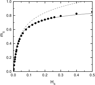
FIG. 1.: The staggered-magnetization curve for $S=1$. Our results (solid line) are compared with DMRG data (circles) and with the NL$\sigma$M results (dotted line) of Refs.[12] and [14], respectively.

where $A=\Delta_{0}\frac{3}{4\pi}\frac{\sinh(\pi S/3)}{S(JS)^{1/2}}$. It is obvious from Eq. (21) that the magnetization saturates to its maximum value of $m_{s}=1$ only asymptotically for $H_{s}\to\infty$. This is consistent with the fact that it is only in that asymptotic limit that a fully polarized Néel state becomes an exact eigenstate of the original Heisenberg Hamiltonian (1), as well as with the fact that our mean-field approach keeps track of the NL$\sigma$M constraint, albeit only on the average.

In Figure 1 we compare, for $S=1$, our staggered-magnetization curve with DMRG data [12] and with the NL$\sigma$M treatment of Ref. [14]. The magnetization curve was obtained by solving numerically Eq. (14) (with $\Lambda$ given by Eq. (18)) and by inserting the resulting $\xi$ into Eq. (15). As already anticipated, the agreement with the DMRG data is excellent over the whole range of fields.

We have also solved Eq. (14) for $S=2$, by fixing again $\Lambda$ via Eq. (18) with the value, specific to $S=2$, $\Delta_{0}=0.0876J$[16]. At present, the staggered-magnetization curve for $S=2$ has not yet been obtained by numerical methods. Given the excellent agreement between our curve and numerical data for $S=1$, we expect that our magnetization curve (shown in Figure 2) will agree with future numerical investigations also in the case $S=2$. Indeed, on general grounds, Haldane’s mapping is expected to work even better when the value of the spin $S$ is increased. Note that the magnetization increases faster with $H_{s}$ (or, equivalently, the staggered susceptibility becomes larger) when the spin $S$ is increased. This is consistent with the fact that, when $S\to\infty$, the system approaches the classical one, which is critical at $T=0$ and $H_{s}=0$. Note also that the value of the zero-field Haldane gap roughly sets the scale of the staggered-magnetization curve.

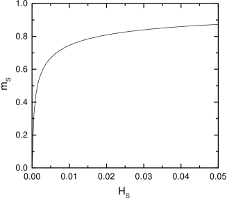
FIG. 2.: The staggered-magnetization curve for S=2.

Introducing an external space and time-dependent source field $\mathbf{J=J(x)}$ and promoting the partition function ${\cal Z}$ to a generating functional ${\cal Z}[{\bf J}]$ obtained by replacing in the original path-integral the Euclidean Lagrangian of Eq. (2) with:

$${\cal L}[{\bf J}]=\frac{1}{2g}\left[\frac{1}{c}\left(\frac{\partial{\bf n}}{\partial\tau}\right)^{2}+c\left(\frac{\partial{\bf n}}{\partial x}\right)^{2}\right]-{\bf n}({\bf x})\cdot{\bf J}({\bf x})\;\;,$$ (22)

the connected Green functions for the staggered field ${\bf n}$:

$$G_{c}^{\alpha,\beta}({\bf x},{\bf x}^{\prime})=\langle{\rm T_{\tau}}[n^{\alpha}({\bf x})n^{\beta}({\bf x}^{\prime})]\rangle-\langle n^{\alpha}({\bf x})\rangle\langle n^{\beta}({\bf x}^{\prime})\rangle$$ (23)

can be obtained by double functional differentiation with respect to the source field as:

$$G_{c}^{\alpha,\beta}({\bf x},{\bf x}^{\prime})=\left.\frac{\delta^{2}\ln{\cal Z}[{\bf J}]}{\delta{\bf J}^{\alpha}({\bf x})\delta{\bf J}^{\beta}({\bf x}^{\prime})}\right|_{{\bf J}=S{\bf H}_{s}}\;\;\;.$$ (24)

The saddle-point analysis can be performed in this case as well. The saddle-point equation reads now:

$$\frac{3}{2}K^{-1}({\bf x},{\bf x}) = 1-\frac{1}{4}\int d{\bf y}d{\bf y}^{\prime}K^{-1}({\bf y},{\bf x})K^{-1}({\bf x},{\bf y}^{\prime})$$ (25)

$$\times {\bf J}({\bf y})\cdot{\bf J}({\bf y}^{\prime})\;\;\;.$$ (26)

This equation will yield in general a space and time-dependent saddle point $\lambda_{sp}=\lambda_{sp}({\bf x})$, which will reduce however to a constant for ${\bf J}=const.=S{\bf H}_{s}$ when, as it can be checked easily, Eq. (26) reproduces our previous Eq. (10). What matters here is the fact that the saddle point will depend quadratically on the source field. From this it follows that the transverse Green functions $G_{xx}({\bf x},{\bf x}^{\prime})=G_{yy}({\bf x},{\bf x}^{\prime})$ do not get any additional contribution from the dependence of $\lambda_{{\rm sp}}$ on ${\bf J}$ (we assume here ${\bf H}_{s}={\hat{z}}H_{s}$) and can be calculated by taking ${\bf J}=S{\bf H}_{s}$ from the beginning. The transverse Green functions are thus still given by the same expression valid for $H_{s}=0$, Eq. (17) where now $\xi$ depends on ${\bf H}_{s}$ via Eq. (14). The transverse gap will be accordingly $\Delta_{\perp}({\bf H}_{s})=\frac{c}{\xi({\bf H}_{s})}$, and in Figure 3 we compared the transverse gap as calculated by this relation with the one obtained by DMRG data. The agreement is again excellent.

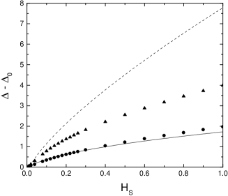
FIG. 3.: Plots of the transverse (solid curve) and longitudinal (dashed curve) gap predicted by the NL$\sigma$M approach, compared with the corresponding DMRG data (circles and triangles, respectively).

In the parallel channel, on the other hand, the dependence of $\lambda_{{\rm sp}}$ on ${\bf J}$ yields additional contributions to the Green functions, which do not allow us to calculate the longitudinal Green functions explicitly. To obtain an estimate for the longitudinal gap we resorted to the so called “single-mode approximation”[14], that is we assumed the gap and susceptibilities to be connected by the same law both in the transverse and parallel channel. It can be readily shown that for an isotropic system, for which the magnetization is directed along the external field, $\chi_{\perp}=\frac{\partial m_{s}^{x}}{\partial H_{s}^{x}}=m_{s}/H_{s}$, while $\chi_{\parallel}=\frac{\partial m^{z}_{s}}{\partial H^{z}_{s}}=\frac{dm_{s}}{dH_{s}}$. From Eq. (15) we thus find $\chi_{\perp}=Sg\xi^{2}/c=Sgc/(\Delta_{\perp})^{2}$. If we assume the same relation to hold also in the parallel channel, $\Delta_{\parallel}$ can be calculated as a derived quantity from the magnetization curve by using $\Delta_{\parallel}=(Sgc/\chi_{\parallel})^{1/2}$. Our data for $\Delta_{\parallel}$ are also shown in Figure 3. The agreement with the DMRG data is definitely worse in this case, and this may attributed to a shortcoming of the single-mode approximation in the longitudinal channel. The complete structure of the Green functions along the lines outlined above in Eqs. (22) and (24) is being presently undertaken, and more extended and complete results will be published elsewhere [17].

In conclusion, we come to a brief comparison between our approach and that of Refs. [13] and [14].

What the two approaches have in common is the starting point, namely the mapping of the original problem onto a NL$\sigma$M, slightly modified by the external staggered field. In the abovemntioned references, however, the authors resolved to relaxing the NL$\sigma$M constraint by replacing it with a polynomial self-interaction of the ${\bf n}$-field, keeping terms in the expansion of the interaction up to eight order. This leads to a (generalized) Ginzburg-Landau-type theory with up to six free parameters which the authors took from previous numerical and Renormalization-Group studies. Their results for the staggered magnetization saturate at a finite value of the staggered field (see Figure 1), which indicates that softening the NL$\sigma$M constraint is inappropriate at high fields. Also, their results for the gaps deviate badly from the DMRG results. All this has been evidenced in Ref. [12] and justifies the negative comments of the authors in that reference, that however should be addressed more to the additional approximations adopted in Refs. [13] and [14] than to the NL$\sigma$M approach itself.

- [1] F.D.M. Haldane, Phys. Rev. Letters 50, 1153 (1983). For a more recent approach, see: D.C. Cabra, P. Pujol and C.von Reichenbach, Phys. Rev. B58,65(1998).
- [2] For a review, see: I. Affleck in: Fields, Strings and Critical Phenomena, E. Brézin and J. Zinn-Justin Eds.,North-Holland, Amsterdam, 1989. Also, for reviews on spin ladders, see: E. Dagotto and T.M. Rice, Science 271, 618 (1996) and: E. Dagotto, cond-mat/9908250.
- [3] The equivalence between two-leg spin- ladders and spin- chains has been shown by: S.R. White, cond-mat/9503104.
- [4] J. Darriet and L.P. Regnault, Solid State Commun. 86, 409(1993); J.F. DiTusa et al., Physica B194-196, 181 (1994) and: L.P. Regnault, I. Zalisnyak, J.P. Renard, and C. Vettier, Phys. Rev. B50, 9174 (1994).
- [5] S.R. White and A. Huse, Phys.Rev. B48, 3844 (1993).
- [6] O.Golinelli, T.Jolicœur and R.Lacaze, Phys. Rev. B50, 3037 (1994).
- [7] I. Affleck, Phys. Rev. B43, 3215 (1991).
- [8] M. Oshikawa, M. Yamanaka and I. Affleck, Phys. Rev. Letters 78, 1984 (1997).
- [9] J.F. DiTusa et al., Phys. Rev. Letters 73, 1857 (1993); K.Kojima et al., Phys. Rev. Letters 74, 3471 (1994); E.García-Matres, J.L. García-Munoz, J.L. Martínez and J. Rodriguez-Carvajal, J. Magn. Magn. Mater. 149, 363 (1995).
- [10] A. Zheludev, J.P. Hill and D.J. Buttrey, Phys. Rev. B54, 7216 (1996).
- [11] A. Zheludev, E. Ressouche, S. Maslov, T. Yokoo, S. Raymond and J. Akimitsu, Phys. Rev. Letters 80, 3630 (1998).
- [12] Jizhong Lou, Xi Dai, Shaojin Qin, Zhaobin Su and Yu Lu, Phys. Rev. B60, 52 (1999).
- [13] S. Maslov and A. Zheludev, Phys. Rev. B57, 68 (1998).
- [14] S. Maslov and A. Zheludev, Phys. Rev. Letters 80, 5786 (1998).
- [15] T. Sakai and H. Shiba, J. Phys. Soc. Jpn. 63, 867 (1994).
- [16] Xiaoqun Wang, Shaojing Qin, Lu Yu, cond-mat/9903035.
- [17] E.Ercolessi, G.Morandi, P.Pieri and M.Roncaglia, in preparation.