[

Spinless fermions and charged stripes at the strong-coupling limit

Abstract

Spinless fermions on a lattice with nearest-neighbor repulsion serve as a toy version Hubbard model, and have a symmetry-broken even/odd superlattice at half-filling. At infinite repulsion, doped holes form charged stripes which are antiphase walls (as noted by Mila in 1994). Exact-diagonalization data for systems up to 36 sites around 1/4 filling, and also for one or two holes added to a stripe of length up to 12, indicate stability of the stripe-array state against phase separation. In the boson version of the model, the same behavior can be stabilized by addition of a four-fermi term.

]

Forty years of study have not yet produced a complete understanding of the phase diagram of the Hubbard model, the simplest nontrivial paradigm of interacting spinfull fermions.[1] The spinless lattice fermion model [2] is a simpler and more tractable analog which retains many Hubbard-model properties, much as the Ising model stands in for the $n$-component magnet in critical phenomena: understanding of the spinless model may provide fresh viewpoints of the Hubbard model, or new tests of known methods. Spinless models also arise naturally for ferromagnetic materials in which one of the spin-split bands is completely full or completely empty, such as magnetite [3] or “half-metallic” manganites [4].

Our aim is to promote the systematic study of this model’s phase diagram, which is almost untouched in the literature [5, 6, 7]. As a beginning, this paper argues that, in the strong-coupling limit, the spinless model possesses a phase with the quantum-fluctuating, hole-rich antiphase domain walls known as “stripes.” Such stripes are an active topic in the Hubbard or $t-J$ models, [8, 9, 10, 11, 12, 13, 14, 15] particularly since stripes were observed in cuprates [16] and seem related to incommensurate correlations found in high-temperature superconductors.

Let us take a square lattice model with Hamiltonian

$${\cal H}=-t\sum_{\langle ij\rangle}(c_{i}{{}^{\dagger}}c_{j}+c_{j}{{}^{\dagger}}c_{i})+V\sum_{\langle ij\rangle}\hat{n}_{i}\hat{n}_{j}$$ (1)

Here $c_{i}{{}^{\dagger}}$ and $c_{i}$ are creation/annihilation operators on site $i$, $\hat{n}_{i}\equiv c{{}^{\dagger}}_{i}c_{i}$, and “$\langle...\rangle$” counts each nearest-neighbor pair once. In most places we will consider hard-core bosons in parallel with fermions [17]. From here on, we take $V/|t|=\infty$ so neighboring particles are simply forbidden, and $t$ is the only energy scale. (This constraint amounts to adopting a hardcore radius just over 1 lattice constant.)

Phase diagram as function of $n$ – Consider first the dilute limit, $n{\lesssim}0.15$. When $V\to\infty$, the Hartree-Fock approximation gives absurd results; in reality the renormalized interaction of two particles is of order $t$ and a Bose or Fermi liquid is expected, as when the on-site repulsion $U\to\infty$ in the Hubbard model [18].

At the other extreme, the dense limit ($n=1/2$, half-filling) admits only the two microstates with the $\sqrt{2}\times\sqrt{2}$ checkerboard pattern, called the “CDW” (“charge-density wave”) order  [5]. An Ising symmetry breaking between even/odd lattices is exhibited, the spinless model’s cartoon of the Heisenberg antiferromagnetic order at half-filling in the large-$U$ Hubbard model.

Stripes in a hard-core model – Now consider light hole doping, $1/2-n\ll 1$. An isolated hole is immobile and gains no hopping energy in the CDW state (see Fig. 1). As Mila [19] observed, a droplet including $\geq$3 holes can fluctuate but is still confined to a circumscribed rectangle with edges along the $45^{\circ}$ directions, since a particle is prevented from hopping away from a CDW domain surface oriented along $\{11\}$ (Fig. 1).

The natural way to dope holes is a “stripe”, an antiphase domain wall with charge 1/2 hole per unit length. This permits hops (arrows in Fig. 1) which implement stripe fluctuations. [19] A single stripe’s path can be parametrized as a unique function $y(x)$ (hopping never generates overhangs). Then $y(x+1)-y(x)=\pm 1$, and the steps up or down can be represented by a string of corresponding ${\uparrow}$ and ${\downarrow}$ arrows. A particle hop has the effect ${\uparrow}{\downarrow}\to{\downarrow}{\uparrow}$ and so the Hamiltonian of a single stripe maps exactly to the spin-1/2 XX chain [19] with exchange $J_{\perp}=-t$ for the X and Y spin components. That model is exactly soluble by a well-known mapping, whereby the up (down) spins map to noninteracting spinless fermions (empty sites), respectively, in one dimension. It follows that the energy of the (coarse-grained) stripe is

$$\int dx[\sigma_{0}+{\frac{1}{2}}K(dy/dx)^{2}+\ldots],$$ (2)

where $\sigma_{0}=-(2/\pi)t$ and the stripe stiffness $K=(\pi/2)t$. As usual, the sound velocity of the stripe’s capillary waves is the Fermi velocity $v=2t/\hbar$ of the 1D noninteracting fermions. Knowing $K$ and $v$ allows us to compute the fluctuations of the Fourier mode at each wavevector $q$, as for any harmonic string: $\langle|y_{q}|^{2}\rangle=\hbar v/2K|q|$. The general result is that one such “Gaussian” quantum-fluctuating stripe has divergent fluctuations,

$$\langle|y(x)-y(0)|^{2}\rangle=(v/2\pi K)\ln|x|+{\rm const},\quad\hbox{as $x\to\infty$}$$ (3)

where $v/2\pi K=2/\pi^{2}$ in this case.

The thermodynamic phase at $1/2-n\ll 1$ could then be an array of stripes [20] all parallel (on average) to either the $\hat{x}$ or $\hat{y}$ axis. They have only a contact interaction, so the array’s long-range order depends on stripe collisions, which surely exist since isolated stripes have divergent fluctuations (eq. (3)).

Prior analytic work [6] suggested that spinless fermions in $d=2$, when doped away from half-filling, develop an incommensurate ordering wavevector slightly off from $(\pi,\pi)$). Expanding around the $d=\infty$ limit,[7] small doping led to coexistence between the half-filled CDW and a slightly incommensurate state (but not at $V/t\to\infty$). We conjecture these incommensurate phases, in $d=2$, consist of stripe arrays. In the hard-core boson model near half-filling, in a regime $0<V/t<\infty$, the uniform CDW phase is asserted to phase-separate upon doping [21]. The dense coexisting state is just as plausible, a priori, to be a stripe array as the phase-separated state that was assumed. [21, 22].

Stability estimates – The key question is whether (or when) the stripe-array is stable, compared to a phase-separated state in which the CDW state and the dilute (=hole-rich) liquid coexist. In the case of the Hubbard model, it was argued that doping invariably leads to phase separation [23] except when it is “frustrated” [8] by the long-range Coulomb force. Contrarily, it was argued that holes in fluctuating stripes may gain more kinetic energy than they would in a phase-separated state [9].

To decide the issue of coexistence, one first plots the energy per site ${E^{\rm liq}}(n)$ and ${E^{\rm sa}}(n)$ for the low-density liquid and the stripe-array, respectively, which should look like Fig. 2 for either fermions or hardcore bosons. We have

$${E^{\rm liq}}(n)=(-4t)n+A_{2}n^{2}+A_{3}n^{3}+\ldots$$ (4)

where the leading coefficient is the bottom of the single-particle band. [24] With increasing density, the energy ${E^{\rm liq}}(n)$ turns upwards and becomes small around $n=0.3$ as the hopping becomes “jammed” (neighbor sites become forbidden due to other adjacent particles). The matrix elements contribute with the same sign in the boson ground state but can’t in the fermion case, so ${E^{\rm liq}}_{\rm fermions}>{E^{\rm liq}}_{\rm bosons}$.

On the other hand, in the conjectured stripe array near half filling,

$${E^{\rm sa}}(n)\approx[\sigma_{0}+\phi(d)](1-2n)$$ (5)

where $\sigma_{0}$ is the energy per unit $x$-length from (2); the second factor is the length of stripe per unit area. The mean stripe separation is $d\equiv(1-2n)^{-1}$, and $\phi(d)$ parametrizes the energy cost per unit length from collisions of adjacent stripes, [15] so $\phi(d)\to 0$ as $d\to\infty$. Thus, the chemical potential in the limit of separated stripes is ${\mu^{*}}\equiv d{E^{\rm sa}}(n)/dn|_{n=1/2}=(4/\pi)t=1.273t$. We emphasize that the form and the leading coefficients in (4) and (5) are the same for fermions and hardcore bosons. [Indeed, the fermion and boson models are identical in the single-stripe sector, since the $V=\infty$ constraint prevents any permutations; this identity extends to the single stripe with one extra hole, in which case only even permutations are accessible [26].]

There are three necessary conditions for the stability of the stripe array: we have strong evidence for each of them, from exact diagonalizations of systems with 20 to 72 sites. [25] These are far too small for direct observation of a fluctuating stripe array, or of the coexistence of the liquid and dense phases; yet they are large enough to yield some of the parameters which the phase diagram can be calculated from. From here on we use units $t\equiv 1$.

The first stability condition is that stripes repel, i.e. $\phi(d)>0$; stripe attraction would suggest instability to a domain of liquid phase, which is scarcely distinguishable from a bundle of self-bound stripes. In both the fermion and boson cases we diagonalized $L\times L^{\prime}$ systems, for $L=4$, and $L^{\prime}=6,8,10$, as well as $L=L^{\prime}=6$, doped with $L$ holes so that two stripes run in the short direction, and thus $d=L^{\prime}/2$. Define a stripe interaction per unit length $\phi_{\rm eff}(L^{\prime}/2)\equiv(E-2{E^{\rm str}}(L))/2L$, where ${E^{\rm str}}(L)$ is the energy of one isolated stripe of finite (even) length $L$. (${E^{\rm str}}(L)$ is calculated exactly using the 1D spinless-fermion representation.) Indeed, $\phi_{\rm eff}(d)$ was positive and (for $L=4$) decreasing with $d$.

Next, a stripe can contain extra holes, [11] which move as quasiparticles with an excitation gap $\Delta$. The second stability condition is

$$\Delta>-{\mu^{*}}$$ (6)

If not, further doping would add holes to existing stripes rather than form new ones, again suggesting a tendency to form phase-separated droplets. From diagonalizations we measured the excitation energy of one added hole, [27] $\Delta(L,L^{\prime})$, with even $L$ and odd $L^{\prime}$ in the range $[4,8]$ for fermions, or $[4,12]$ for bosons; as mentioned above, this is strictly independent of statistics [26]. From this we extrapolated, first $L^{\prime}\to\infty$ using $\Delta(L,L^{\prime})=\Delta(L)+A_{\Delta}(L)e^{-L^{\prime}/l(L)}$ and then $L\to\infty$ using $\Delta(L)=\Delta+B_{\Delta}/L$. We found $\Delta=-0.65(5)$, which comfortably satisfies (6).

We also analyzed the two-hole energy $\Delta_{2}(L)$, for $L=4,6,8,10$ only; with two holes, the $L$ dependence is more like $1/2^{L}$ than $1/L$. Extrapolating to $L=\infty$, yielded $\Delta_{2}=-1.42(7)$ for bosons and $-1.44(9)$ for fermions. Note $\Delta_{2}-2\Delta\approx-0.1$, i.e. hole binding is insignificant when $L\leq 10$; we think it is a real effect in a large system, since holes on a stripe can be collected into a (hole-free) vertical segment of the stripe. (Since the stripe’s $90^{\circ}$ kinks cost energy, an array of parallel stripes will still be the thermodynamic phase in a large system.)

The third condition is the crucial one: as shown in Fig. 2, the dense phase coexisting with the liquid must not be the CDW, which would preempt a stripe-array phase. That is,

$${\mu^{*}}>{\mu^{\rm LC}}.$$ (7)

where ${\mu^{\rm LC}}$ is the slope of the trial liquid-CDW tie-line tangent to ${E^{\rm liq}}(n)$ and passing through $(n=1/2,E=0)$.

To test (7), the equation of state ${E^{\rm liq}}(n)$ is required. We exactly diagonalized all rectangular lattices with $L,L^{\prime}\geq 4$ and $LL^{\prime}=20$ to 36 sites, and with occupation in the range $0.20\leq n<0.3$, and fitted the results to (4). We obtained $(A_{2},A_{3})\simeq(9.45\pm 0.6,5\pm 2)$ for bosons and $(11.25\pm 0.6,-1\pm 2)$ for fermions. This implies ${\mu^{\rm LC}}_{\rm bosons}=1.33(2)$ and ${\mu^{\rm LC}}_{\rm fermions}=1.25(2)$. (Here the errors are estimated by varying the subset of data used for the fit.) For either bosons or fermions, coexistence with the CDW would occur at $n_{c}\approx 0.24$.

Hence, stripes are unstable in the boson case and (very likely) stable in the fermion case, but close enough to the boundary in either case that the balance can be tipped either way by the small perturbation ${\tilde{t}}_{c}$, discussed later.

Exotic states? – Like the Hubbard model, the spinless fermion model may be extended by adding other hopping terms to the Hamiltonian, which might stabilize additional phases. Many of these terms have the form

$$-{\tilde{t}}_{x}(c{{}^{\dagger}}_{j}c_{i}+c{{}^{\dagger}}_{i}c_{j})\hat{n}_{k},$$ (8)

where $(i,j,k)$ are three different sites arranged as in Fig. 3, and $x$ is “$a$”, “$b$”, or “$c$” for the hops shown in the corresponding parts of Fig. 3. For example, when $V$ is large but finite, hops are possible to a neighbor’s neighbor with ${\tilde{t}}_{a}={\tilde{t}}_{b}=-t^{2}/V$ as in Fig. 3(a) and (b), analogous to similar terms of order $t^{2}/U$ when the $t$-$J$ model is derived from the Hubbard model. This spinless analog of the $t$-$J$ model, in which virtual states with neighbor pairs are projected out, will be the natural starting point to study phenomena at large (but not infinite) $V$, e.g. the mobility of lone holes.

In the fermion model, one could artificially take ${\tilde{t}}_{b}\gg t$ (analogous to $J\gg t$ in the $t$-$J$ model); then the term Fig. 3 (b) naturally favors superconductivity. Namely, fermions form tightly bound $p$-wave pairs, separated by $\sqrt{2}$; these composite bosons hop with bandwidth $8{\tilde{t}}_{b}$, and Bose-condense in the usual fashion. Thus ${\tilde{t}}_{b}$ is analogous to negative $U$ in the Hubbard model, in that superconductivity is put in “by hand”. But it is a plausible speculation that, in the highly correlated liquid at $n\approx 0.25$, BCS superconductivity appears even with ${\tilde{t}}_{b}\ll t$.

Finally, consider the hopping ${\tilde{t}}_{c}$ of Fig. 3 (c) which just modifies the amplitude of already possible hops. This tends to stabilize (destabilize) stripes according to whether ${\tilde{t}}_{c}$ has the same (opposite) sign as $t$, since every allowed hop in a stripe is surrounded by particles on all four possible “$k$” sites. (Compare Fig. 3(c) with Fig. 1). Hence the stripe energy $\sigma_{0}$ and ${\mu^{*}}$ get multiplied by a factor $(1+4{\tilde{t}}_{c}/t)$. On the other hand, assuming that each “$k$” site is about $1/3$ occupied in the liquid at $n=0.25$, it follows that ${E^{\rm liq}}(n)$ is multiplied by about $(1+4{\tilde{t}}_{c}/3t)$. If so, the critical perturbation where ${\mu^{\rm LC}}={\mu^{*}}$ (so the stripe phase appears or vanishes) is only ${\tilde{t}}_{c}/t\approx 0.02$ for bosons or $-0.007$ for fermions, using our values of ${\mu^{\rm LC}}$ quoted above.

Discussion – To establish the occurrence of stripes in the $V=\infty$ system, we addressed, by exact diagonalizations, (i) stripe-stripe interactions; (ii) the energy of a single hole, as well as hole-hole interactions, on a stripe; and (iii) the medium density liquid regime. (iv) hole-hole interactions on a stripe The enormous reduction of Hilbert space due to the nearest-neighbor exclusion (at $V=\infty$), as well as the lack of spin, permits numerical explorations at system sizes much larger than would be possible in the Hubbard model – vital not just for studying stripes, but any microscopically inhomogenous states. Monte Carlo simulation of the stripe phase is straightforward for the hardcore boson case. [22] Boson results are valid for fermions too, when the stripe separation $d$ is large and the density of “extra holes” on each stripe is low, since particles do not exchange in this limit [26]. As for the fermion case, the new “meron-cluster” Monte Carlo algorithm cancels the sign problem for a limited class of models including spinless fermions, but not the basic Hubbard model [28].

The ultimate aim of microscopic simulations should be to extract macroscopic parameters, e.g. the stripe stiffness $K$ or the stripe contact repulsion. This is more straightforward than in the spin-full (Hubbard or $t$-$J$) case, where the inter-stripe domains contain gapless spin-wave excitations [14]. These parameters may be input to analytic explorations of the interesting anisotropic conductivity of the quantum-fluctuating stripe array [29], also simpler in the spinless case.

More broadly, it is a challenge to test for the exotic phases we mentioned in connection with Fig. 3. In the medium-density regime $n\approx 0.2$, strong correlations of some sort are essential to minimize the hopping energy. These might be prosaic, e.g. a $\sqrt{5}\times\sqrt{5}$ superlattice, but the following possibilities are realizable, in principle, even in a spinless model: (i) orbital magnetism (spontaneous circulating currents around plaquettes); (ii) $p$-wave superconductivity (see the speculations on Fig. 3(b)); or (iii) the analog of spin-charge separation, the spinon being replaced by a spinless particle that carries Fermi statistics [30]. If it transpires that such states are hard to stabilize without spin, that would shed additional light on the Hubbard model; contrariwise, if they are stabilized, they may be easier to study in the spinless case, free from any background of low-energy spin excitations.

A crude comparison may be made of the spinless-fermion model with the infinite-$U$ Hubbard model in the dilute regime. In that case, each fermion excludes one site (its own) from half of the other fermions, not counting the exclusion built in by Fermi statistics. In the present spinless model each fermion excludes four sites from all other fermions, so in a sense the hole-rich metal phase is “jammed” eight times more effectively than in the Hubbard case. We expect, then, that kinetic-energy-stabilized stripes are far more robust in the present model than in the large-$U$ Hubbard case. In fact they are practically marginal in the present model, so this encourages the opinion that stripes are not stable in the short-range Hubbard (or $t$–$J$) model.

We acknowledge support by the National Science Foundation under grants DMR-9981744 and PHY94-07194. C. L. H. thanks R. McKenzie, G. Uhrig, D. Scalapino, D. Khomski, M. Troyer, and G. G. Batrouni for helpful discussions.

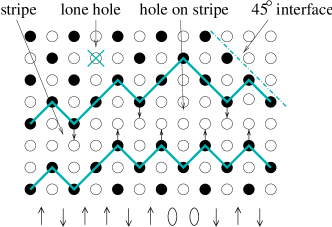
FIG. 1.: Hard-core particles (filled circles) must form a checkerboard at half-filling in the $V=\infty$ limit. No hopping is possible by the lone hole ($\times$ mark) or $45^{\circ}$ interface (dot-dash line), but hopping is easy (arrows) along the stripe. The stripe’s edges are shown by shaded lines and its spin-chain representation is below. One extra hole is shown on the stripe.

FIG. 2.: Schematic of energy $E(n)$ as a function of filling $n$, assuming ${\mu^{\rm LC}}<{\mu^{*}}$. Dotted segments are metastable states. Thin lines are drawn with slopes ${\mu^{*}}$ and ${\mu^{\rm LC}}$.

FIG. 3.: More hopping terms allowed in the $V=\infty$ Hilbert space, from site $i$ to site $j$ when site $k$ is occupied (Eq. (8). These terms might modify the phase diagram (see text).

REFERENCES

- [1] P. Fazekas, Lecture Notes on Electron Correlation and Magnetism (World Scientific, Singapore, 1999).
- [2] W. Kohn, Phys. Rev. Lett. 19, 789 (1967).
- [3] J. R. Cullen and E. Callen, Phys. Rev. Lett. 26, 236-8 (1971).
- [4] R. A. de Groot et al, Phys. Rev. Lett. 50, 2024 (1983).
- [5] The simulation of this model by J. E. Gubernatis et al, Phys. Rev. B 32, 103 (1985), was limited to the half-filled case, with finite and nonzero temperature.
- [6] G. Murthy and R. Shankar, J. Phys. Condens. Matt. 7, 9155 (1995).
- [7] G. S. Uhrig and R. Vlaming, Phys. Rev. Lett. 71, 271 (1993); G. S. Uhrig and R. Vlaming, Physica B 206 & 207, 694 (1995).
- [8] (a) V. J. Emery, S. A. Kivelson, and H. Q. Lin, Phys. Rev. Lett. 64, 475 (1990); (b) V. J. Emery and S. A. Kivelson, Physica C 209, 597 (1993).
- [9] P. Prelovšek and I. Sega, Phys. Rev. B 49, 15241 (1994).
- [10] J. Zaanen, M. L. Horbach, and W. van Saarloos, Phys. Rev. B 53, 8671 (1996).
- [11] C. Nayak and F. Wilczek, Phys. Rev. Lett. 78, 2465 (1997).
- [12] H. Eskes et al, Phys. Rev. B 58, 6963 (1998). The lattice strings in their model may become “smooth”, with nondivergent fluctuations in (3); that might occur in our model with Hamiltonian (1) if or if (8) is added.
- [13] S. R. White and D. J. Scalapino, Phys. Rev. Lett. 81, 3227 (1998).
- [14] L. P. Pryadko et al, Phys. Rev. B60, 7541 (1999).
- [15] For an argument on the form of , see J. Zaanen Phys. Rev. Lett. 84, 753 (2000).
- [16] J. M. Tranquada et al, Phys. Rev. Lett. 73, 1003 (1994).
- [17] The hard-core boson model maps to a spin-1/2 quantum antiferromagnet, in which occupied sites correspond to up spins, the XY spin components have coupling , and the components have coupling . But this is not helpful in our limit, since the spin model Hamiltonian also contains a magnetic field of order .
- [18] J. Kanamori, Prog. Theor. Phys. 30, 275 (1963); V. M. Galitskii, Sov. Phys. JETP 34, 104 (1958).
- [19] F. Mila, Phys. Rev. B 49, 14047 (1994). Mila actually considered a spinfull extended Hubbard model but the spin freedom is trivial in the case, since all assignments of fermion spins are degenerate eigenstates.
- [20] Quantum-fluctuating strings in two dimensions, as represented by a path integral, map to classical fluctuating surfaces in three dimensions. The classical behaviors are reviewed in, e.g., M. E. Fisher, J. Stat. Phys. 34, 667 (1984)
- [21] G. G. Batrouni et al Phys. Rev. Lett. 74, 2527 (1995); G. G. Batrouni and R. T. Scalettar, Phys. Rev. Lett. 84, 1599 (2000).
- [22] A quantum Monte Carlo simulation at of the hardcore boson system (with ), by G. G. Batrouni (personal communication), showed superfluid at , , coexisting with a dense (presumably 2-stripe) state at , consistent with the phase diagram presented here, and with our exact diagonalization result for the same . (This aspect ratio strongly favors stripe states.)
- [23] P. Visscher, Phys. Rev. B 10, 943 (1974).
- [24] For bosons as , one would expect in Eq. (4). See M. Schick, Phys. Rev. A3, 1067 (1971).
- [25] N. G. Zhang and C. L. Henley, unpublished.
- [26] C. L. Henley, in preparation.
- [27] depends slightly on because holes can be transferred from one stripe to the next stripe.
- [28] S. Chandrasekharan and U.-J. Wiese, Phys. Rev. Lett. 83, 3116 (1999).
- [29] T. Noda, H. Eisaki, and S, Uchida, Science 286, 265 (1999).
- [30] T. Senthil and M. P. A. Fisher, preprint (cond-mat/9910224), and personal communications.