Density of the Fisher zeroes for the Ising model

Abstract

The density of the Fisher zeroes, or zeroes of the partition function in the complex temperature plane, is determined for the Ising model in zero field as well as in a pure imaginary field $i\pi/2$. Results are given for the simple-quartic, triangular, honeycomb, and the kagomé lattices. It is found that the density diverges logarithmically at points along its loci.

1 Introduction

In the analyses of lattice models in statistical mechanics such as the Ising model, the partition function is often expressed in the form of a polynomial in variables such as the external magnetic field and/or the temperature. Since properties of a polynomial are completely determined by its roots, a knowledge of the zeroes of the partition function yields all thermodynamic properties of the system. Particularly, if the zeroes lie on a certain locus, a knowledge of its density distribution along the locus is equivalent to the obtaining of the exact solution of the problem.

For the Ising model with ferromagnetic interactions, we have the remarkable Yang-Lee circle theorem [1] which states that all partition function zeroes lie on the unit circle $|z|=1$ in the complex $z=e^{2L}$ plane, where $L$ is the reduced external magnetic field $(wesetkT=1)$. However, the density of the Yang-Lee zeroes on the unit circle, a knowledge of which is equivalent to solving the Ising model in a nonzero magnetic field, is known only for the Ising model in one dimension.

Fisher [2] has proposed that it is also meaningful to consider partition function zeroes in the complex temperature plane. Indeed, he showed that for the zero-field Ising model on the simple quartic lattice with nearest-neighbor reduced interactions $K$, the partition function zeroes lie on two circles

$$|\tanh K\pm 1|=\sqrt{2}$$ (1)

in the thermodynamic limit. He further showed that the known logarithmic singularity of the specific heat follows from the fact that the density vanishes linearly near the real axis. Subsequently, the Fisher loci has been determined for the infinite triangular lattice [3], and for finite simple-quartic lattices which are self-dual [4]. Stephenson [6] has also evaluated the density distribution on the circles in terms of a Jacobian. However, the explicit expressions of the density function of the Fisher zeroes do not appear to have been heretofor evaluated.

In this paper we complete the picture by evaluating the density function. We deduce the explicit expressions for the density of Fisher zeroes for the simple-quartic, triangular, honeycomb, and kagomé lattices. Density of the Fisher zeroes for the Ising model in a pure imaginary field $L=i\pi/2$ are also obtained.

2 The simple-quartic lattice

It is well-known that the bulk solution of spin models with short-range interactions is independent of the boundary conditions. For the Ising model on the simple-quartic lattice, we shall take a particular boundary condition introduced by Brascamp and Kunz [5] for which the location of the Fisher zeroes is known for any finite lattice. This permits us to take a a well-defined and unique bulk limit, thus avoiding a difficulty encountered in the consideration of the Ising model on a torus [6].

Consider an $M\times 2N$ simple-quartic lattice with cylindrical boundary conditions in the $N$ direction and fixed boundary conditions along the two edges of the cylinder. The $2N$ boundary spins on each of the two edges of the cylinder have fixed fields $\cdots++++++\cdots$ and $\cdots+-+-+-\cdots$, respectively. This is the Brascamp-Kunz boundary condition [5]. Brascamp and Kunz showed that the partition function of this Ising model is precisely

$$Z_{M,2N}(K)=2^{2MN}\prod_{1\leq i\leq N}\prod_{1\leq j\leq M}\biggl{[}1+z^{2}-z(\cos\theta_{i}+\cos\phi_{j})\biggr{]},$$ (2)

where

$$z=\sinh 2K,\hskip 28.45274pt\theta_{i}=(2i-1)\pi/{2N},\hskip 28.45274pt\phi_{j}=j\pi/(M+1).$$ (3)

The per-site “free energy” in the bulk limit is then evaluated as

$$f = \lim_{M,N\to\infty}{1\over{2MN}}\ln\ Z_{M,2N}(K)$$ (4)

$$= {1\over 2}\ln(4z)+{1\over 8\pi^{2}}\int_{-\pi}^{\pi}d\theta\int_{-\pi}^{\pi}d\phi\ \ln[z+z^{-1}-(\cos\theta+\cos\phi)]$$

$$= {1\over 2}\ln(4z)+{1\over 2\pi^{2}}\int_{0}^{\pi}d\theta\int_{0}^{\pi}d\phi\ \ln[z+z^{-1}-2\cos u\cos v],$$

where $u=(\theta+\phi)/2,v=(\theta-\phi)/2$ and we have made use of the fact that the integrands are $2\pi$-periodic.

The partition function (2) has zeroes at the $2MN$ solutions of

$$z+z^{-1}=\cos\theta_{i}+\cos\phi_{j},\ \ \ 1\leq i\leq N;1\leq j\leq M.$$ (5)

The following lemma and corollaries are now used to determine the loci of the zeroes:

Lemma: The regime $-2\leq z+z^{-1}\leq 2$ of the complex $z$ plane, where $z+z^{-1}=$ real, is the unit circle $|z|=1$.

Proof: The Lemma follows from the fact that, by writing $z=re^{i\theta}$, we have

$$z+z^{-1}=\biggl{(}r+{1\over r}\biggr{)}\cos\theta+i\biggl{(}r-{1\over r}\biggr{)}\sin\theta,$$ (6)

so that $z+z^{-1}=$ real implies either $r=1$ or $\theta=$ integer $\times\pi$. In the latter case we have $|z+z^{-1}|=|r+r^{-1}|>2$, which contradicts the assumption, unless $r=1$. It follows that we have always $r=1$, or $|z|=1$. Q.E.D.

Corollary 1: The regime $-a\leq z+z^{-1}\leq b$, where $a,b>2$, $z+z^{-1}=$ real, of the complex $z$ plane is the union of the unit circle $|z|=1$ and segments $z_{-}(-a)\leq x\leq z_{+}(-a)$ and $z_{-}(b)\leq x\leq z_{+}(b)$ of the real axis, where $z_{\pm}(b)=(b\pm\sqrt{b^{2}-4})/2$.

Corollary 2: The regime $-a\leq z+z^{-1}\leq b$, where $a,b>2$, $z+z^{-1}=$ real, of the complex $z$ plane, is the regime $|w|=1$ in the complex $w$ plane, where $w$ is the solution of the equation

$$w+w^{-1}={4\over{a+b}}\biggl{(}z+z^{-1}+{{a-b}\over 2}\biggr{)}.$$ (7)

Corollary 1 is established along the same line as in the proof of the lemma, and Corollary 2 is a consequence of the lemma since, by construction, we have $-2\leq w+w^{-1}\leq 2$.

Returning to the partition function (2), since the right-hand side of (5) is real and lies in $[-2,2]$, it follows from the Lemma that the $2MN$ zeroes of (2) all lie on the unit circle $|\sinh 2K|=1$, a result which can also be obtained by simply setting the argument of the logarithm in the bulk free energy (4) equal to zero. The usefulness of this simplified procedure has been pointed out by Stephenson and Couzens [3] for the Ising model on a torus. But since the zeroes are not easily determined in that case when the lattice is finite, they termed the argument as “hand-waving”. Here, the argument is made rigorous by the use of the Brascamp-Kunz boundary condition. From here on, therefore, We shall adopt this simpler approach in all subsequent considerations.

We now proceed to determine the density of the zero distribution. Let the number of zeroes in the interval $[\alpha,\alpha+d\alpha]$ be $2MNg(\alpha)d\alpha$ such that

$$\int_{0}^{2\pi}g(\alpha)d\alpha=1$$ (8)

and

$$f={1\over 2}\ln(4z)+\int_{0}^{2\pi}d\alpha\ g(\alpha)\ \ln(z-e^{i\alpha}).$$ (9)

It is more convenient to consider the function $R(\alpha)=\int_{0}^{\alpha}g(x)dx$ where $2MNR(\alpha)$ gives the total number of zeroes in the interval $[0,\alpha]$ such that

$$g(\alpha)={d\over{d\alpha}}R(\alpha).$$ (10)

On the circle $|z|=1$ writing $z=e^{\alpha}$ and setting the argument of the logarithm in the third line of (4) equal to zero, we find $\alpha$ determined by

$$\cos\alpha=\cos u\cos v,\hskip 28.45274pt0\leq\{u,v\}\leq\pi.$$ (11)

Now if $\alpha_{i}$ is a solution, so are $-\alpha_{i}$ and $\pi-\alpha_{i}$, hence we have the symmetry

$$g(\alpha)=g(-\alpha)=g(\pi-\alpha).$$ (12)

It is therefore sufficient to consider only $0\leq\{\alpha,u,v\}\leq\pi/2$.

   

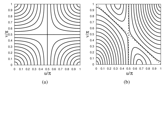
Figure 1: Constant-$\alpha$ contours in the $u$-$v$ plane. (a). The contour (11) for the simple-quartic lattice. Straight lines correspond to $\alpha=\pi/2$. (b). The contour (23) for the triangular lattice. Broken lines correspond to $\alpha=2\cos^{-1}(1/3)$.

The constant-$\alpha$ contours of 11 are constructed in Fig. 1(a) and are seen to be symmetric about the lines $u,v=\pm\pi/2$ in each of the 4 quadrants. Now from (3) we see that zeroes are distributed uniformly in the $\{\theta,\phi\}$-, and hence the $\{u,v\}$-plane. It follows that $R(\alpha)$ is precisely the area of the region

$$\cos\alpha>\cos u\cos v,\hskip 28.45274pt0\leq\{\alpha,u,v\}\leq\pi/2,$$ (13)

normalized to $R(\pi/2)=1/4$. This leads to the expression

$$R(\alpha)={\frac{1}{\pi^{2}}}\int_{0}^{\alpha}\cos^{-1}\Bigg{(}{\frac{\cos\alpha}{\cos x}}\Bigg{)}dx.$$ (14)

Using (10) and after some reduction, we obtain the following explicit expression for the density of zeroes,

$$g(\alpha)=R^{\prime}(\alpha)={\frac{|\sin\alpha|}{\pi^{2}}}K(\sin\alpha),$$ (15)

where $K(k)=\int_{0}^{\pi/2}dt(1-k^{2}\sin^{2}t)^{-1/2}$ is the complete elliptic integral of the first kind. The density (15), which possesses an unexpected logarithmic divergence at $\alpha=\pm\pi/2$, is plotted in Fig. 2(a). For small $\alpha$, we have $g(\alpha)\approx|\alpha|/2\pi$. As pointed out by Fisher [2], it is this linear behavior at small $\alpha$ which leads to the logarithmic divergence of the specific heat.

We can also deduce the density of zeroes on the two Fisher circles (1) which we write as

$$\tanh K\pm 1=\sqrt{2}e^{i\theta}.$$ (16)

The angles $\alpha$ and $\theta$ are related by,

$$e^{i\alpha}=\pm\Big{(}{{\sqrt{2}\mp e^{-i\theta}}\over{\sqrt{2}\mp e^{i\theta}}}\Big{)}$$ (17)

so that the mapping from $\alpha$ to $\theta$ is 1 to 2. This leads to the result

$$g(\theta)={{g(\alpha)}\over 2}\Bigg{|}{{d\alpha}\over{d\theta}}\Bigg{|}.$$ (18)

Let the density of zeroes be $g_{\pm}(\theta)$ for the two circles (16). Then, using (17) we find

$$g_{+}(\theta) = g_{-}(\pi-\theta)$$ (19)

$$= \biggl{(}{k\over\pi^{2}}\biggr{)}\Bigg{|}{1-\sqrt{2}\cos\theta\over 3-2\sqrt{2}\cos\theta}\Bigg{|}K(k),$$

where

$$k={2|\sin\theta|(\sqrt{2}-\cos\theta)\over 3-2\sqrt{2}\cos\theta}.$$ (20)

The density (19) is plotted as Fig. 2(b). Note that the divergence in the density distribution in (14) is removed in (19). The points $\alpha=\pm\pi/2$ in $g(\alpha)$ is mapped onto the points $\theta=\pm(\pi/2\pm\pi/4)$ in $g_{\pm}(\theta)$. We have $g_{+}(\pi/4)=g_{-}(3\pi/4)=0$, and for small $\theta$ we find

$$g_{\pm}(\theta)=\Big{(}{{3\pm 2\sqrt{2}}\over{\pi}}\Big{)}|\theta|.$$ (21)

Here, again, the linear behavior of $g_{+}(\theta)$ at $\theta=0$ leads to the logarithmic singularity of the specific heat.

It is also of interest to consider zeroes of the Ising model in the Potts variable $x=(e^{2K}-1)/\sqrt{2}$. In the complex $x$ plane it is known [7] that the partition function zeroes are on two unit circles centered at $x=1$ and $x=-\sqrt{2}$. We find the density along the two circles to be, respectively, $g_{-}(\theta)$ and $g_{+}(\theta)$.

   

Figure 2: Density of partition function zeroes for the simple-quartic lattice. (a). $g(\alpha)$ given by (15). (b). $g_{+}(\theta)$ given by (19).

3 The triangular lattice

For the triangular Ising model with nearest-neighbor interactions $K$, the free energy assumes the form [8, 9]

$$f = C+{1\over 8\pi^{2}}\int_{-\pi}^{\pi}d\theta\int_{-\pi}^{\pi}d\phi\ln\biggl{[}z+z^{-1}+1-[\cos\theta+\cos\phi+\cos(\theta+\phi)]\biggr{]},$$ (22)

$$= C+{1\over{2\pi^{2}}}\int_{0}^{\pi}du\int_{0}^{\pi}dv\ln\Big{[}z+z^{-1}+2-2\cos u(\cos u+\cos v)\Big{]},$$

where $C=[\ln(4z)]/2$, $z=(e^{4K}-1)/2$, and we have introduced variables $u=(\theta+\phi)/2,v=(\theta-\phi)/2$. Now the value of the sum of the three cosines in (22) lies between $-3/2$ and $3$. It then follows from Corollary 1 that in the complex $z$ plane the zeroes lie on the union of the unit circle $|z|=1$ and the line segment $[-2,-1/2]$ of the real axis, a result first obtained by Stephenson and Couzens [3].

The density of the zero distribution can now be computed in the same manner as described in the preceding section. For $z$ on the unit circle we write $z=e^{i\alpha}$. Then $\alpha$ is determined by

$$\cos\alpha=-1+\cos u(\cos u+\cos v),\hskip 28.45274pt0\leq\{u,v\}\leq\pi,$$ (23)

and $R(\alpha)$ is the area of the region

$$\cos\alpha>-1+\cos u(\cos u+\cos v).$$ (24)

Clearly, we have the symmetry $g_{\rm cir}(\alpha)=g_{\rm cir}(\pi-\alpha)$ and we need only to consider $0\leq\alpha\leq\pi$.

From a consideration of the constant-$\alpha$ contours of 23 shown in Fig. 1(b), we obtain after some algebra the result

$$g_{\rm cir}(\alpha)={|\sin\alpha|\over{\pi^{2}\sqrt{A(\alpha)}}}K(k),$$ (25)

where $A(\alpha)=(5+4\cos\alpha)^{1/2}$ and

$$k^{2} = F[A(\alpha)]$$

$$F(x) \equiv {1\over 16}\Big{(}{3\over x}-1\Big{)}(1+x)^{3}.$$ (26)

Particularly, for small $\alpha$, we find $g_{\rm cir}(\alpha)\approx|\alpha|/2\sqrt{3}\pi$.

In a similar fashion we find, on the line segment $z\in[-2,-1/2]$, we write $z=-e^{\lambda}$ and obtain

$$g_{\rm line}(\lambda)={|\sinh\lambda|\over\pi^{2}k\sqrt{B(\lambda)}}K(k^{-1}),\hskip 28.45274pt-\ln 2\leq\lambda\leq\ln 2,$$ (27)

where $B(\lambda)=[5-4\cosh\lambda]^{1/2}$ and

$$k^{2}=F[B(\lambda)].$$ (28)

In contrast to the case of the simple-quartic lattice, the density of zeroes is everywhere finite. Specifically, we have $g_{\rm cir}(\pi)=g_{\rm line}(0)=0$, and $g_{\rm line}(\pm\ln 2)=\sqrt{3}/2\pi$. The densities (25) and (27) are plotted in Fig. 3.

   

Figure 3: Density of partition function zeroes for the triangular lattice. (a). $g_{\rm cir}(\alpha)$ given by (25). (b). $g_{\rm line}(z)$ given by (27).

Matveev and Shrock [16] have discussed zeroes of the triangular Ising model in the complex $u=e^{-4K}$ plane, for which the zeroes are distributed on the union of the circle

$$u={1\over 3}(2e^{i\alpha}-1),\qquad-\pi<\alpha\leq\pi,$$ (29)

and the line segment

$$-\infty<u\leq-{1\over 3}.$$ (30)

Using our results we find the respective densities

$$g_{\rm cir}(\alpha)={|\sin\phi|\over{9\pi^{2}}}[C(\alpha)]^{7/2}K(k),$$ (31)

where $C(\alpha)=3(5-4\cos\phi)^{-1/2}$, $k^{2}=F[C(\alpha)]$, and

$$g_{\rm line}(u)=\Bigg{|}{(1+u)(1-3u)\over 4\pi^{2}u^{2}(1-u)^{2}k\sqrt{D(u)}}\Bigg{|}\ K(k^{-1}),$$ (32)

where $D(u)=\sqrt{(1+3u)/u(1-u)}$ and $k^{2}=F[D(u)]$. At the end point we have $g_{\rm line}(-1/3)=9\sqrt{3}/8\pi$.

The density of zeroes assumes a simpler form if we use Corollary 2 to map all zeroes onto a unit circle in the complex $w$ plane, where $w$ is root of the quadratic equation

$$w+w^{-1}={4\over 7}\biggl{(}z+z^{-1}+{3\over 4}\biggr{)},$$ (33)

and $z=(e^{4K}-1)/2$. For $w$ on the unit circle, we write $w=e^{i\alpha}$ and find in analogous to (13) that $R(\alpha)$ is the area of the region

$$\cos\alpha>{1\over 9}\Big{[}8\cos u(\cos u+\cos v)-7\Big{]}.$$ (34)

Using the contours shown in Fig. 1(b), we obtain

$$R(\alpha) = {\frac{1}{\pi^{2}}}\int_{0}^{\phi_{0}}\cos^{-1}\Bigg{[}{\frac{9\cos\alpha+7}{8\cos{\phi}}}-\cos{\phi}\Bigg{]}d\phi,\hskip 28.45274pt\alpha\in[0,\alpha_{0}]$$ (35)

$$= {\frac{1}{2}}-{\frac{1}{\pi^{2}}}\int_{\phi_{0}}^{\phi_{1}}\cos^{-1}\Bigg{[}{\frac{9\cos\alpha+7}{8\cos{\phi}}}-\cos{\phi}\Bigg{]}d\phi,\quad\alpha\in[\alpha_{0},\pi],$$

where $\alpha_{0}=2\cos^{-1}(1/3)$ and

$$\phi_{0} = \cos^{-1}\Bigg{[}{\frac{3}{2}}\cos{\frac{\alpha}{2}}-{\frac{1}{2}}\Bigg{]}$$

$$\phi_{1} = \pi-\cos^{-1}\Bigg{[}{\frac{3}{2}}\cos{\frac{\alpha}{2}}+{\frac{1}{2}}\Bigg{]},\quad{\rm for}\quad\cos{\frac{\alpha}{2}}\leq{\frac{1}{3}}.$$ (36)

Note that we have $R(\alpha_{0})=3/8$, $R(\pi)=1/2$.

Finally, using (10), we obtain

$$g(\alpha) = {\frac{9\sin\alpha}{8\pi^{2}}}\int_{0}^{\phi_{0}}{\frac{d\phi}{\sqrt{(\cos^{2}\phi-\cos^{2}\phi_{0})(\Delta^{2}-\cos^{2}\phi)}}},\hskip 22.76228pt\alpha\in[0,\alpha_{0}]$$ (37)

$$= {\frac{9\sin\alpha}{8\pi^{2}}}\int_{\phi_{0}}^{\phi_{1}}{\frac{d\phi}{\sqrt{(\cos^{2}\phi-\cos^{2}\phi_{0})(\cos^{2}\phi_{1}-\cos^{2}\phi)}}},\quad\alpha\in[\alpha_{0},\pi],$$

where $\Delta=[1+3\cos({\alpha}/{2})]/2$. After some manipulation and making use of integral identities (A1) and (A2) derived in the Appendix, we obtain

$$g(\alpha) = {\frac{3\sqrt{3}}{8\pi^{2}}}\Big{|}\sin\alpha\Big{|}\sqrt{\sec{\frac{\alpha}{2}}}K(k),\quad\alpha\in[0,\alpha_{0}]$$ (38)

$$= {\frac{3\sqrt{3}}{8\pi^{2}}\Bigg{|}{\sin\alpha\over k}\Bigg{|}\sqrt{\sec{\frac{\alpha}{2}}}}K(k^{-1}),\quad\alpha\in[\alpha_{0},\pi]$$

where

$$k^{2}={\frac{1}{16}}(\sec{\frac{\alpha}{2}}-1)\Big{(}1+3\cos{\frac{\alpha}{2}}\Big{)}^{3}.$$ (39)

Note that $g(\alpha)$ diverges logarithmically at $\alpha=\pm\alpha_{0}$.

4 Simple-quartic Ising model in a field $i\pi/2$

The two-dimensional Ising model can be solved when there is an external magnetic field $i\pi/2$. The solution for the simple-quartic lattice was first given by Lee and Yang [10] and a rigorous derivation of which was given later by McCoy and Wu [11]. In 1988 Lin and Wu [12] gave a general prescription for writing down the solution of the Ising model in a field $i\pi/2$ by transcribing the solution in a zero field. The most general known solution of the Ising model in a field $i\pi/2$ is a model with a generalized checkerboard type interactions [13]. We consider in this section the case of the simple-quartic lattice.

For the simple-quartic lattice Lee and Yang [10] gave the free energy in a field $i\pi/2$ as

$$f=i{\pi\over 2}+C+{1\over 16\pi^{2}}\int_{-\pi}^{\pi}d\theta\int_{-\pi}^{\pi}d\phi\ln[z+z^{-1}+2-4\cos\theta\cos\phi],$$ (40)

where $C=(\ln\sinh 2K)/2,z=e^{-4K}$. Setting the argument of the logarithm in (40) equal to zero we have $-6\leq z+z^{-1}\leq 2$ and hence from Corollary 2 we see that in the complex $z$ plane zeroes of the partition function lie on the unit circle $|z|=1$ and the line segment $-3-2\sqrt{2}\leq z\leq-3+2\sqrt{2}$ of the real axis.

On the unit circle $|z|=1$ we write $z=e^{i\alpha}$ and find the density

$$g_{\rm cir}(\alpha)={|\sin\alpha|\over 2\pi^{2}}K(k),$$ (41)

where

$$k^{2}=(3+\cos\alpha)(1-\cos\alpha)/4.$$ (42)

On the line segment, we write $z=-e^{\lambda}$ with $-2\ln(1+\sqrt{2})\leq\lambda\leq 2\ln(1+\sqrt{2})$, we find the density

$$g_{\rm line}(\lambda)={|\sinh\lambda|\over 2\pi^{2}}K(k),$$ (43)

where

$$k^{2}=(3-\cosh\lambda)(1+\cosh\lambda)/4.$$ (44)

At the end points we have $g_{\rm line}(\pm 2\ln(1+\sqrt{2}))=1/\sqrt{2}\pi$. The density functions (41) and (43) are plotted in Fig. 4.

   

Figure 4: Density of partition function zeroes for the simple-quartic lattice Ising model in a field $i\pi/2$. (a). $g_{\rm cir}(\alpha)$ given by (41). (b). $g_{\rm line}(z)$ given by (43).

5 Triangular Ising model in a field $i\pi/2$

The solution for the triangular model in a field $i\pi/2$ was first obtained in [12] by applying a transformation in conjunction with the solution of a staggered 8-vertex model. Here, for completeness, we present an alternate and more direct derivation.

   

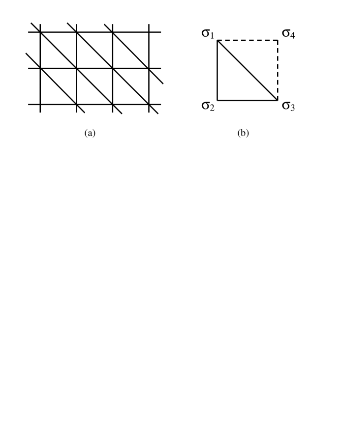
Figure 5: (a). The triangular lattice. (b). A unit cell.

Consider a triangular Ising lattice of $N$ sites whose sites are arranged as shown in Fig. 5(a). After making use of the identity $e^{i\pi\sigma/2}=i\sigma$, the partition function assumes the form

$$Z_{N}=i^{N}\sum_{\sigma_{i}=\pm 1}\prod_{\rm nn}e^{K\sigma_{i}\sigma_{j}}\prod_{j}\sigma_{j}$$ (45)

where the first product is over all nearest neighbors, and the second product over all sites. Now it is known that the triangular Ising model can be mapped into an 8-vertex model on the dual of the square lattice [14], also of $N$ sites. However, in order to properly treat the factor $\prod_{j}\sigma_{j}$ in (45), we need to divide the $N$ “cells” of the lattice, where a cell is shown in Fig. 5(b), into two sublattices, $A$ and $B$, and associate two $\sigma_{j}$’s to each cell belonging to one sublattice, say, $B$. This permits us to rewrite (45) as

$$Z_{N}=i^{N}\sum_{\sigma_{i}=\pm 1}\ \prod_{\rm cells}W_{\rm stg}(\sigma_{1},\sigma_{2},\sigma_{3},\sigma_{4})$$ (46)

where $W_{\rm stg}(\sigma_{1},\sigma_{2},\sigma_{3},\sigma_{4})$ is a staggered Boltzmann weight given by

$$W_{\rm stg}(\sigma_{1},\sigma_{2},\sigma_{3},\sigma_{4}) = e^{K(\sigma_{1}\sigma_{2}+\sigma_{2}\sigma_{3}+\sigma_{3}\sigma_{1})}\hskip 42.67912pt{\rm for\>\>}A$$ (47)

$$= (\sigma_{1}\sigma_{2})e^{K(\sigma_{1}\sigma_{2}+\sigma_{2}\sigma_{3}+\sigma_{3}\sigma_{1})}\hskip 14.22636pt{\rm for\>\>}B.$$

The 8-vertex weights are

$$\{\omega_{1},\cdots,\omega_{8}\} = \{e^{3K},e^{-K},e^{-K},e^{-K},e^{-K},e^{-K},e^{-K},e^{3K}\}$$

$$\{\omega_{1}^{\prime},\cdots,\omega_{8}^{\prime}\} = \{e^{3K},-e^{-K},-e^{-K},e^{-K},e^{-K},-e^{-K},e^{-K},-e^{3K}\}.$$ (48)

Furthermore, from the mapping convention of Fig. 1 of [15], we see that the mapping between the spin and 8-vertex configurations is 2 to 1. This leads to

$$Z_{N}=2i^{N}Z_{N}(\{\omega\},\{\omega^{\prime}\}),$$ (49)

which is an exact equivalence between $Z_{N}$ and the partition function $Z_{N}(\{\omega\},\{\omega^{\prime}\})$ of the staggered 8-vertex model.

Now the weights (48) satisfy the free-fermion condition [14] for which $Z_{N}(\{\omega\},\{\omega^{\prime}\})$ has already been evaluated [15]. Using Eq. (19) of [15] and after some reduction, one obtains the following expression for the per-site free energy,

$$f=i{\pi\over 2}+C+{1\over 4\pi^{2}}\int_{0}^{\pi}d\theta\int_{0}^{\pi}d\phi\ln\Big{[}(1+e^{4K})^{2}+4\cos\phi(\cos\theta+\cos\phi)\Big{]},$$ (50)

where $C=[\ln(2\sinh 2K)]/2$. As a result, the partition function zeroes are located at

$$(1+e^{4K})^{2}=-4\cos\phi(\cos\theta+\cos\phi),\hskip 28.45274pt0\leq\{\theta,\phi\}\leq\pi.$$ (51)

It is therefore convenient to consider the $z=e^{4K}$ plane. Since

$$-8\leq(1+e^{4K})^{2}\leq 1,$$ (52)

using the Lemma we find that the zeroes are on the union of the segment $-2\leq z\leq 0$ of the real axis and the line segment $z=-1+iy$, $-2\sqrt{2}\leq y\leq 2\sqrt{2}$. The density of zeroes can be similarly determined. On the segment $z\in[-2,0]$ of the real axis, we find

$$g(z)=\Bigg{|}{(1+z)\over 2\pi^{2}k\sqrt{E(z)}}\Bigg{|}\ K(k^{-1}),$$ (53)

where $E(z)=\sqrt{-z(2+z)}$ and $k^{2}=F[E(z)]$. Particularly, we have $g(0)=g(-2)=1/\sqrt{3}\pi$ and $g_{(}-1)=0$. On the line segment $z=-1+iy$, we find

$$g(y)=\Bigg{|}{y\over 2\pi^{2}\sqrt{H(y)}}\Bigg{|}\ K(k),$$ (54)

where $H(y)=\sqrt{1+y^{2}}$ and $k^{2}=F[H(y)]$. Particularly, we have $g(0)=0$ and $g(\pm 2\sqrt{2})=1/\sqrt{6}\pi$. These results are plotted in Fig. 6.

   

Figure 6: Density of partition function zeroes for the triangular Ising model in a field $i\pi/2$. (a). $g(z)$ given by (53). (b). $g(y)$ given by (54).

we remark that in the complex $x=e^{-4K}$ plane considered in [16], the segment $-2\leq z\leq 0$ of the real axis maps onto $-\infty\leq x\leq-1/2$ while the line segment $z=-1+iy$, $-2\sqrt{2}\leq y\leq 2\sqrt{2}$, is mapped onto the circular arc $x^{-1}={1\over 2}(-1+e^{i\theta})$, $\theta_{0}=\tan^{-1}(4\sqrt{2}/7)\leq|\theta|\leq\pi$. The density of zeroes on the arc is found to be

$$g_{\rm arc}(\theta)={(1+\cos\theta)^{2}\over 2\pi^{2}\sqrt{I(\theta)}|\sin^{3}\theta|}\ K(k),$$ (55)

where $I(\theta)=[2(1+\cos\theta)]^{1/2}/|\sin\theta|$ and $k^{2}=F[B(\theta)]$. The densities at the end points of the arc are $g_{\rm arc}(\pm\theta_{0})=3\sqrt{3}/2\sqrt{2}\pi$.

6 The honeycomb and kagomé lattices

The partition function of an Ising model on a planar lattice with interactions $K$ is proportional to the partition function on the dual lattice with interactions $K^{*}$ [17], where $K$ and $K^{*}$ are related by

$$e^{-2K^{*}}=\tanh K.$$ (56)

Consequently, their partition function zeroes coincide when expressed in terms of appropriate variables. Now the honeycomb and triangular lattices are mutually dual, it follows that for the honeycomb lattice with interactions $K$, in the complex

$$z={1\over 2}(e^{4K^{*}}-1)=(\cosh 2K-1)^{-1}$$ (57)

plane, zeroes of the partition function coincides with those of the triangular lattice partition function (22).

For the honeycomb Ising model in an external field $i\pi/2$, the free energy can be obtained from that in a zero field via a simple transformation [12, 16]. Writing the partition function in the form of (45) and replacing the product $\prod_{i}\sigma_{i}$ by $\prod_{i}\sigma_{i}^{3}$, it is clear that, besides the factor $i^{N}$, the partition function is the same as that in a zero field with the replacement

$$e^{K(\sigma_{i}\sigma_{j}-1)}\to(\sigma_{i}\sigma_{j})e^{K(\sigma_{i}\sigma_{j}-1)},$$ (58)

or, equivalently, $e^{2K}\to-e^{2K}$. It follows that in the complex

$$z=(-\cosh 2K-1)^{-1}$$ (59)

plane, the zeroes coincide with those of the triangular lattice partition function (22).

The Ising model on the kagomé lattice with interactions $K$ can be mapped to that on an honeycomb lattice with interactions $J$, by applying a star-triangle transformation followed by a spin decimation. The procedure, which is standard [18] and will not be repeated here, leads to the relation

$$e^{2J}=({e^{4K}+1})/2.$$ (60)

As a result, we conclude that, in the complex

$$z=(\cosh 2J-1)^{-1}=2(1-\tanh 2K)/\tanh^{2}2K$$ (61)

plane, zeroes of the kagomé partition function coincides with those of the triangular lattice partition function (22). The evaluation of the kagomé partition function in an external field $i\pi/2$ remains unresolved, however.

References

[1] C. N. Yang and T. D. Lee, Statistical theory of equations
of states and phase transitions I. Theory of
condensation, Phys. Rev. 87, 404-409 (1952).
[2] M. E. Fisher, The Nature of Critical Points, in:
Lecture Notes in Theoretical Physics,
vol. 7c, edited by W. E. Brittin,
(University of Colorado Press, Boulder, 1965), pp. 1-159.
[3] J. Stephenson and R. Couzens,
Partition function zeros for the two-dimensional
Ising model, Physica A 129, 201-210 (1984).
[4] W. T. Lu and F. Y. Wu, Partition function zeroes of a self-dual
Ising model, Physica A 258, 157-170 (1998).
[5] H. J. Brascamp and H. Kunz, Zeroes of the partition
function for the Ising model in the complex temperature plane,
J. Math. Phys. 15, 65-66 (1974).
[6] J. Stephenson, Partition function zeros for the two-dimensional
Ising model. II, Physica A 136, 147-159 (1986).
[7] C. N. Chen, C. K. Hu, and F. Y. Wu,
Partition function zeros of the square lattice Potts model,
Phys. Rev. Lett. 76, 169-172 (1996).
[8] R. M. F. Houtappel, Order-disorder in hexagonal lattice,
Physica 16, 425-455 (1950).
[9] G. H. Wannier, Antiferromagnetism: The triangular
Ising Nnt, Phys. Rev. 79, 357-364 (1950).
[10] T. D. Lee and C.N. Yang, Statistical theory of equations of
state and phase transitions. II. Lattice gas and Ising model,
Phys. Rev. 87, 410-419 (1952).
[11] B. M. McCoy and T. T. Wu, Theory of Toeplitz determinants
and the spin correlations of the two-dimensional Ising model. II.
Phys. Rev. 155, 438-452 (1967).
[12] K. Y. Lin and F. Y. Wu, Ising model in
the magnetic field , Int. J. Mod. Phys. B 4, 471-481 (1988).
[13] F. Y. Wu, Two-dimensional Ising model with crossing and
four-spin interactions and a magnetic field ,
J. Stat. Phys. 44, 455-463 (1986).
[14] C. Fan and F. Y. Wu, General lattice model of phase transitions,
Phys. Rev. B 2, 723-733 (1970).
[15] C. S. Hsue, K. Y. Lin, and F. Y. Wu,
Staggered eight-vertex model, Phys. Rev. B 12, 429-437 (1975).
[16] V. Matveev and R. Shrock, Complex-temperature properties
of the two-dimensional Ising model for nonzero
magnetic field, Phys. Rev. E 53, 254-267 (1996).
[17] F. Y. Wu and Y. K. Wang, Duality transformation in a many
component spin model, J. Math. Phys. 17, 439-440 (1976).
[18] I. Syozi, Transformation of Ising Models,
in Phase Transition and Critical Phenomena,
vol. 1, edited by C. Domb and M. Green
(Academic Press, London, 1970) 269-329.
[19] I. S. Gradshteyn and I. M. Ryzhik, Table of Integrals,
Series and Products, 5th edition (Academic Press, New York, 1994).