Quasiparticle Spectrum of $d$-wave Superconductors
in the Mixed State

Abstract

The quasiparticle spectrum of a two-dimensional $d$-wave superconductor in the mixed state, $H_{c1}\ll H\ll H_{c2}$, is studied both analytically and numerically using the linearized Bogoliubov–de Gennes equation. We consider various values of the “anisotropy ratio” $v_{F}/v_{\Delta}$ for the quasiparticle velocities at the Dirac points, and we examine the implications of symmetry. For a Bravais lattice of vortices, we find there is always an isolated energy-zero (Dirac point) at the center of the Brillouin zone, but for a non-Bravais lattice with two vortices per unit cell there is generally an energy gap. In both of these cases, the density of states should vanish at zero energy, in contrast with the semiclassical prediction of a constant density of states, though the latter may hold down to very low energies for large anisotropy ratios. This result is closely related to the particle-hole symmetry of the band structures in lattices with two vortices per unit cell. More complicated non-Bravais vortex lattice configurations with at least four vortices per unit cell can break the particle-hole symmetry of the linearized energy spectrum and lead to a finite density of states at zero energy.

I Introduction

In the past few years several key experiments have demonstrated that the order parameter in high-temperature superconductors has $d$-wave symmetry rather than the conventional $s-$wave symmetry found in low-temperature superconductors [2]. This fact has strong implications for the low-temperature thermodynamics of these systems, because the $d$-wave symmetry implies the existence of points on the Fermi surface where the gap function vanishes. At these points the bulk quasiparticle spectrum will be gapless and these states will be occupied even at very low temperature.

High-$T_{c}$ superconductors are extreme Type-II superconconductors and in a magnetic field larger than $H_{c1}$ develop a vortex lattice. The geometry of this vortex lattice has been investigated via small angle neutron scattering [3], scanning tunneling microscopy [4, 5] and magnetic decoration [6] in YBa₂Cu₃O₇ (YBCO) and Bi₂Sr₂CaCu₂O₈ (Bi2212). In YBCO twinned single crystals the vortex lattice in a magnetic field of 6 T parallel to the $c$ axis looks like a skewed square lattice with an angle between primitive vectors of about $77^{\circ}$ [4]. Low-field magnetic decoration studies of Bi2212 between 70 G and 120 G parallel to the $c$ axis [6] find a vortex lattice very close to a hexagonal one.

We have studied the quasiparticle spectrum of a $d$-wave superconductor in the vortex lattice within the framework of the Bogoliubov–de Gennes equation. The main question we have addressed is whether the spectrum becomes gapped in the presence of a magnetic field $H_{c1}\ll H\ll H_{c2}$ and more generally what the energy spectrum looks like. This question was previously approached via numerical simulation of a tight-binding model [7, 8] and semiclassical analysis [9]. Gor’kov and Schrieffer [10] and, in a more recent preprint using different arguments, Anderson [11] predicted that the quasiparticle spectrum of a $d$-wave superconductor in a magnetic field $H\ll H_{c2}$ is characterized by broadened Landau levels with energy levels

$$E_{n}=\pm\hbar\omega_{H}\sqrt{n},\ \ n=0,1,\ldots$$ (1)

where $\omega_{H}=\sqrt{2\omega_{c}\Delta_{0}/\hbar}$. Here $\omega_{c}=|eH|/mc$ is the cyclotron frequency and $\Delta_{0}$ is the maximum superconducting gap. A key assumption of Gor’kov and Schrieffer and of Anderson, however, was to neglect the spatially dependent superfluid velocity which has been shown to strongly mix Landau levels by Mel’nikov [12].

Recently a preprint by Franz and Tešanović [13] has given new insight into the problem. They introduced a gauge transformation that takes into account the supercurrent distribution and the magnetic field on an equal footing. In this way they map the original problem onto that of diagonalizing a Dirac Hamiltonian in an effective periodic vector and scalar potential with vanishing magnetic flux in the unit cell. Employing the Franz-Tešanović transformation, we were able to tackle the problem of understanding the band structure of this system, via both analytic and numerical methods.

Our analysis will be limited to the spectrum at low energies, in the case where the magnetic field is very small compared to $H_{c2}$. In this case the distance between the vortices is large compared to their diameter, and we can ignore contributions to the spectrum from inside the vortex cores. The quasiparticle states of interest to us are then constructed from excitations close to the nodes of the energy gap of the zero-field spectrum, and we can ignore mixing between different nodes. Thus we analyze the effects of the magnetic field and vortex lattice in a model where the zero field spectrum consists of four independent anisotropic Dirac cones. (We assume that the magnetic field itself is uniform in the sample, which is appropriate for a bulk superconductor provided that $H\gg H_{c1}$, but extends to even smaller fields for a very thin sample.)

A very important numerical parameter in the problem is the anisotropy ratio $\alpha_{D}=v_{F}/v_{\Delta}$. Here $v_{F}$ is the Fermi velocity, while $v_{\Delta}=\Delta_{0}/p_{F}$ is the quasiparticle velocity parallel to the Fermi surface, so the ratio $\alpha_{D}$ measures the anisotropy of the quasiparticle velocities at each Dirac point, in zero field. From angle-resolved photoemission spectroscopy and thermal conductivity measurements, the value of $\alpha_{D}$ for high-$T_{c}$ superconductors turns out to be about 14 for YBCO [14] and 20 for Bi2212 [14, 15]. Conceptually, however, it is useful to consider the entire range of possible values for $\alpha_{D}$, including the “isotropic case” $\alpha_{D}=1$. This is particularly useful because we find that certain features of the spectrum, such as energy gaps can become extremely small for large values of the anisotropy, and therefore become difficult to resolve numerically.

Since each vortex in a superconductor carries only carry half of the normal flux quantum $\Phi_{0}=hc/|e|$, it is necessary to choose a unit cell with an even number of vortices, so that the electron wavefunctions are single valued. Thus, if the vortices sit on a Bravais lattice with one vortex per unit cell, it is necessary to use a double unit cell, containing two vortices, in order to carry out the analysis. On the other hand, if the vortices sit on a non-Bravais lattice, with two vortices per unit cell, one can use directly the unit cell of the vortex lattice.

Some key features of the quasiparticle band structure may be noted by looking at Figs. 3-5 below, which give results of our numerical diagonalization (discussed in Section VI) for a square Bravais lattice, rotated by $45^{\circ}$ from the quasiparticle anisotropy axis, with relatively small anisotropy ratio $1\leq\alpha_{D}\leq 4$. One striking feature is the presence of band crossings both at zero and finite energy, regardless of the value of the anisotropy ratio $\alpha_{D}$. At least for relatively small anisotropy, the level crossings seem to be limited to the $\Gamma$ and M point, as defined in Fig. 1. These band crossings are particularly interesting because in the absence of some special symmetries, we would expect their probability to vanish for a two-dimensional Hamiltonian with broken time-reversal symmetry, as is discussed in more detail in Section VIII.

We have studied the role played by various symmetries of the Hamiltonian both to simplify our numerical computations and to try to understand why band crossings are allowed at some isolated points in the magnetic Brillouin zone. In particular, we focused on zero-energy states, as their existence changes qualitatively the thermodynamic functions of the system, at very low temperatures. For the lattices described above, we find exact particle-hole symmetry, both numerically and analytically, at each point of the magnetic Brillouin zone, as can be seen from the plotted band structures and is further discussed in Section V. Doing perturbation theory calculations described in Section VII, we also found that a crucial role is played by the Bravais nature of the vortex lattice. This symmetry, together with particle-hole symmetry is directly responsible for the spectrum staying gapless in the presence of a magnetic field. To prove this, we considered, both in perturbation theory and by numerical diagonalization, what happens if we deform the vortex lattice so that the distance between the $A$ and $B$ sublattices $2R_{0}$ defined in Fig. 1 is not 1/2 of the distance between two flux lines belonging to the same sublattice, measured along the diagonal. We found that particle-hole symmetry still exists at each point, separately, of the Brillouin zone but that, generally, gaps open up both at the $\Gamma$ and M points, as can be seen in Fig. 6. This result will be discussed in more detail in Section IX.

Another important question is whether there are any further zero-energy modes in addition to the ones at the $\Gamma$ point. This is a very delicate question to address numerically because it is hard to distinguish small gaps from real zero-energy eigenvalues, both because of finite numerical accuracy and, more importantly, because of finite grid-size effects. The latter can be particularly troublesome when dealing with lattice fermions as will be discussed at the beginning of Section VI. In numerical calculations, as noted by Franz and Tešanović, it appears that for anisotropies of the order of 15, there are two lines in the Brillouin zone where the quasiparticle energy vanishes. Based on our symmetry analysis, however, we conclude that there actually remains a very small energy gap all along these lines, both for the case of a Bravais lattice and for a non-Bravais lattice with two vortices per unit cell. On the other hand, we find that for “rectangular” vortex lattices, isolated energy zeroes are allowed along the $\Gamma$X symmetry line (or -X$\Gamma$, by inversion symmetry).

Different conclusions are reached if one allows for more complicated lattice structures, for example considering four vortices per unit cell. In this case it is possible to have superfluid velocity distributions without a center of inversion symmetry leading to non particle-hole symmetric energy spectra as shown in Fig. 7. For large enough anisotropy, there is nothing that prevents lines of energy zeroes from appearing, and the density of states can become finite at zero energy.

The scaling laws for thermodynamic functions computed by Volovik [16] within the semiclassical theory, and by Simon and Lee [17] in a framework closer to our approach, have been tested experimentally (see for example [18]). It is of interest to determine the relation between the semiclassical approximation and the full quantum mechanical spectrum. We have extracted a density of states from the band structures we computed for square vortex lattices and, contrary to the semiclassical prediction of a constant density of states at zero energy, we find a linearly vanishing density of states at low-energy for anisotropy ratio $\alpha_{D}\leq 4$, as shown in Figs. 3-5. Because of the previous discussion on the non-existence of lines of energy zeroes, we are led to believe that this result holds for any value of the anisotropy ratio as long as the vortex lattice has one or two vortices per unit cell. However the semiclassical approximation may be valid down to extremely low energies, when $\alpha_{D}$ is large.

In Section X we study the crossover between the semiclassical and quantum mechanical regions. There are two relevant energy scales which we call $E_{1}$ and $E_{2}$. For $E>E_{1}$ the density of states is qualitatively identical to the bulk density of states in the absence of a magnetic field, although there are still noticeable features induced by van Hove singularities of the band structure in the vortex lattice. Below $E_{1}$, the presence of a magnetic field can be accounted for within a semiclassical approximation, all the way down to an energy scale $E_{2}$ where a full quantum mechanical calculation becomes necessary.

We compare our numerically determined energy scales $E_{1}$ and $E_{2}$ with the crossover scales introduced by Kopnin and Volovik [19, 16] (see also [20]) $E_{1}\approx\hbar v_{F}/d$ and $E_{2}^{KV}\approx\hbar v_{\Delta}/d$, where $d$ is the average distance between vortices. While we agree with their expression for $E_{1}$, we notice that for large anisotropy our numerical analysis indicates that, at least for the geometries considered here, $E_{2}$ should go to zero much faster than $1/\alpha_{D}$. (The precise functional dependence of $E_{2}$ on the anisotropy ratio $\alpha_{D}$ will be the object of a paper currently in preparation.)

The two energies $E_{1}$ and $E_{2}^{KV}$ can also be written as $E_{1}\approx T_{c}\sqrt{H/H_{c2}}$ and $E_{2}^{KV}\approx E_{1}(T_{c}/E_{F})=(T_{c}^{2}/E_{F})\sqrt{H/H_{c2}}$. Experimentally, taking $v_{F}=2.5\times 10^{7}\mbox{cm/s}$ [15] we find that $E_{1}/(k_{B}\sqrt{H})=30\>\mathrm{K/T}^{1/2}$ and $E_{2}^{KV}/(k_{B}\sqrt{H})=2\>\mathrm{K/T}^{1/2}$ for both YBCO and Bi2212, to a good approximation. Recent specific heat [18] and especially low temperature thermal conductivity [21] experiments have been performed in the regime $E<E_{2}^{KV}$ and still show good agreement with the semiclassical predictions, which also seems to suggest that the right crossover scale between the quantum mechanical and semiclassical regime is much smaller than $E_{2}^{KV}$, for large anisotropy ratios. Note that the Landau level energy scale (1) of Gor’kov and Schrieffer and of Anderson is approximately the geometric mean of $E_{1}$ and $E^{KV}_{2}$.

For $E>E_{1}$, the density of states is linear in energy with superimposed sharp peaks (logarithmic van Hove singularities) and the slope is the same as the one in zero magnetic field. When $E_{2}<E<E_{1}$, we are in the regime where the semiclassical theory predicts a constant density of states. This region shrinks as one lowers the anisotropy ratio $\alpha_{D}$, and disappears entirely in the isotropic limit $\alpha_{D}=1$ as is apparent by looking at Fig. 3. In the very low-energy limit $E<E_{2}$, the semiclassical theory breaks down and the density of states has to be computed through the quantum mechanical spectrum. We find that for $E\ll E_{2}$ the density of states is linear and vanishes at zero energy, for the Bravais latitce.

To summarize the structure of the paper, the model Hamiltonian is discussed in Sections II-IV. An analysis of particle-hole symmetry follows in Section V. In Section VI we describe the numerical methods and results of the band structure calculation for a Bravais vortex lattice, while in Sections VII-VIII we study the low-energy states in perturbation theory. More general vortex lattices with two and four vortices per unit cell are considered in Section IX. In Section X, we focus on the density of states and compare it to the semiclassical predictions. Conclusions follow in Section XI.

II Linearized Bogoliubov–de Gennes equation

In a spatially inhomogeneous system, the standard approach to the description of the quasiparticle spectrum is provided by the Bogoliubov–de Gennes equation [22]. For an arbitrary gap operator (i.e. not necessarily $s-$wave), it reads ${\cal H}_{\mbox{BdG}}\psi=E\psi$ where $\psi=(u,v)^{T}$ is a Nambu 2-spinor whose components are the particlelike and holelike part of the quasiparticle wave function, respectively. The Bogoliubov–de Gennes operator ${\cal H}_{\mbox{BdG}}$ we will consider is [17]

$${\cal H}_{\mbox{BdG}}=\left(\begin{array}[]{cc}\displaystyle\frac{(\mbox{\boldmath$p$}-\frac{e}{c}\mbox{\boldmath$A$})^{2}}{2m}-E_{F}&\hat{\Delta}\\ \hat{\Delta}^{*}&\displaystyle-\frac{(\mbox{\boldmath$p$}+\frac{e}{c}\mbox{\boldmath$A$})^{2}}{2m}+E_{F}\end{array}\right),$$ (2)

where $E_{F}$ is the Fermi energy and $m$ is the electron effective mass. Notice that we are neglecting the self-consistent interaction potential [22] (analogous to the Hartree–Fock potential in the normal phase) and any disorder potential. The gap operator acts on components of the wave function as $\hat{\Delta}g(\mbox{\boldmath$r$})=\int d\mbox{\boldmath$r$}^{\prime}\,\Delta_{d}(\mbox{\boldmath$r$},\mbox{\boldmath$r$}^{\prime})g(\mbox{\boldmath$r$}^{\prime})$. For a $d_{xy}$ superconductor, the gap operator can be expressed as $\hat{\Delta}=\frac{1}{p_{F}^{2}}\{p_{x},\{p_{y},\Delta(\mbox{\boldmath$r$})\}\}$ where $\Delta(\mbox{\boldmath$r$})=\Delta_{0}e^{i\phi(\mbox{\boldmath$\scriptstyle r$})}$ and the brackets represent symmetrization $\{a,b\}=\frac{1}{2}(ab+ba)$. We choose this orientation instead of the more conventional $d_{x^{2}-y^{2}}$ purely for notational simplicity; results do not depend on this choice.

In the absence of a magnetic field, there are four points on the Fermi surface at $\mbox{\boldmath$p$}=(\pm p_{F},0)$ and $\mbox{\boldmath$p$}=(0,\pm p_{F})$ where the gap vanishes. If we are interested in the low-energy properties of the quasiparticle excitation spectrum, we can linearize the Bogoliubov–de Gennes equation around one of these points. This procedure is justified because we are considering magnetic fields $H\ll H_{c2}$ and so the inverse magnetic length is much smaller than $k_{F}$. We can choose to linearize around $\mbox{\boldmath$p$}=(0,p_{F})$ writing the wave function $\psi=e^{ik_{F}y}\tilde{\psi}$. The Bogoliubov–de Gennes equation will read $(\tilde{\cal H}_{\mbox{lin}}+\tilde{\cal H}_{\mbox{rest}})\tilde{\psi}=E\tilde{\psi}$, with $\tilde{\cal H}_{\mbox{lin}}$ the leading linearized term

$$\tilde{\cal H}_{\mbox{lin}}=\left(\begin{array}[]{cc}v_{F}(p_{y}-\frac{e}{c}A_{y})&\frac{1}{p_{F}}\{p_{x},\Delta(\mbox{\boldmath$r$})\}\\ \frac{1}{p_{F}}\{p_{x},\Delta^{*}(\mbox{\boldmath$r$})\}&-v_{F}(p_{y}+\frac{e}{c}A_{y})\end{array}\right),$$ (3)

where $v_{F}=p_{F}/m$ is the Fermi velocity and $\tilde{\cal H}_{\mbox{rest}}$ is the remaining piece, which we will disregard being smaller by ${\cal O}\left(\frac{1}{k_{F}d}\right)$. Notice that the linearized eigenvalue problem $\tilde{\cal H}_{\mbox{lin}}\tilde{\psi}=E\tilde{\psi}$ is gauge covariant, so the linearized spectrum will be gauge invariant.

III Franz–Tešanović gauge transformation

Following Franz and Tešanović [13] we can eliminate the phase factor $e^{i\phi(\mbox{\boldmath$\scriptstyle r$})}$ from the off-diagonal components of the Bogoliubov–de Gennes equation performing the singular gauge transformation

$${\cal H}_{\mbox{lin}} \to \tilde{\cal H}_{\mbox{lin}}=U^{-1}{\cal H}_{\mbox{lin}}U,$$ (4)

$$U = \left(\begin{array}[]{cc}e^{i\phi_{A}(\mbox{\boldmath$\scriptstyle r$})}&0\\ 0&e^{-i\phi_{B}(\mbox{\boldmath$\scriptstyle r$})}\end{array}\right)$$ (7)

where $\phi(\mbox{\boldmath$r$})=\phi_{A}(\mbox{\boldmath$r$})+\ \phi_{B}(\mbox{\boldmath$r$})$. $\phi_{A}(\mbox{\boldmath$r$})$ and $\phi_{B}(\mbox{\boldmath$r$})$ are the contributions to the phase coming from the vortex sublattices $A$ and $B$ respectively, as defined in Fig. 1 and will be computed later in the paper.

The gauge transformed Bogoliubov–de Gennes operator is

$$\tilde{\cal H}_{\mbox{lin}} = \left(\begin{array}[]{cc}v_{F}p_{y}&v_{\Delta}p_{x}\\ v_{\Delta}p_{x}&-v_{F}p_{y}\end{array}\right)$$ (10)

$$+ m\left(\begin{array}[]{cc}v_{F}v^{A}_{sy}&\frac{v_{\Delta}}{2}(v^{A}_{sx}-v^{B}_{sx})\\ \frac{v_{\Delta}}{2}(v^{A}_{sx}-v^{B}_{sx})&v_{F}v^{B}_{sy}\end{array}\right),$$ (13)

where $v_{\Delta}=\Delta_{0}/p_{F}$ and the superfluid velocities corresponding to the $A$ and $B$ sublattices are defined as

$$\mbox{\boldmath$v$}^{\mu}_{s}=\frac{1}{m}(\hbar\nabla\phi_{\mu}-\frac{e}{c}\mbox{\boldmath$A$}),\ \ \mu=A,B.$$ (14)

The operator (13) describes the dynamics of a free Dirac particle in a periodic potential. We can take advantage of the periodicity of the potential rewriting our spinors in Bloch form

$$\left(\begin{array}[]{c}u_{\mbox{\boldmath$\scriptstyle k$}}\\ v_{\mbox{\boldmath$\scriptstyle k$}}\end{array}\right)=e^{i\mbox{\boldmath$\scriptstyle k$}\cdot\mbox{\boldmath$\scriptstyle r$}}\left(\begin{array}[]{c}U_{\mbox{\boldmath$\scriptstyle k$}}\\ V_{\mbox{\boldmath$\scriptstyle k$}}\end{array}\right)$$ (15)

where the functions $U_{\mbox{\boldmath$\scriptstyle k$}}(\mbox{\boldmath$r$})$ and $V_{\mbox{\boldmath$\scriptstyle k$}}(\mbox{\boldmath$r$})$ are themselves periodic on the unit cell shown in Fig. 1 and the effective Hamiltonian acting on the Bloch spinors $(U,V)^{T}$ is

$${\cal H} = \left(\begin{array}[]{cc}v_{F}(p_{y}+\hbar k_{y})&v_{\Delta}(p_{x}+\hbar k_{x})\\ v_{\Delta}(p_{x}+\hbar k_{x})&-v_{F}(p_{y}+\hbar k_{y})\end{array}\right)$$ (18)

$$+ m\left(\begin{array}[]{cc}v_{F}v^{A}_{sy}&\frac{v_{\Delta}}{2}(v^{A}_{sx}-v^{B}_{sx})\\ \frac{v_{\Delta}}{2}(v^{A}_{sx}-v^{B}_{sx})&v_{F}v^{B}_{sy}\end{array}\right).$$ (21)

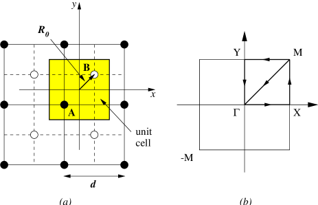
FIG. 1.: (a) A and B sublattices and vortex lattice unit cell. (b) The corresponding magnetic Brillouin zone.

IV Order parameter spatial distribution

The last ingredient we need to determine the quasiparticle spectrum is the order parameter spatial distribution in the vortex lattice. The Bogoliubov–de Gennes method should in principle be used as a set of equations to be solved self-consistently, thus finding the quasiparticle spectrum and wavefunctions, and the spatially varying order parameter distribution. As stated in the introduction, however, we restrict ourselves to the case where the vortex core size is small compared to the spacing between vortices. Thus, we take the magnitude of the order parameter $\Delta_{0}$ to be constant everywhere except at the vortex sites, where it vanishes. We also assume that the magnetic field is constant in the sample. The phase $\phi(\mbox{\boldmath$r$})$ of the gap function $\Delta(\mbox{\boldmath$r$})=\Delta_{0}e^{i\phi(\mbox{\boldmath$\scriptstyle r$})}$ is then obtained by minimizing a simplified Ginzburg-Landau free energy functional[23], which has the form

$$F=\mbox{const}\times\int d^{2}r\,\left|\nabla\phi(\mbox{\boldmath$r$})-\frac{2e}{\hbar c}\mbox{\boldmath$A$}(\mbox{\boldmath$r$})\right|^{2}$$ (22)

where we have taken $e$ to be negative. The phase of the order parameter in the Landau gauge $A_{x}=-By$, $A_{y}=0$ is then given by

$$\nabla\phi(\mbox{\boldmath$r$})=\lim_{\gamma\to 0}\sum_{\alpha}\frac{\hat{z}\times(\mbox{\boldmath$r$}-\mbox{\boldmath$r$}_{\alpha})}{|\mbox{\boldmath$r$}-\mbox{\boldmath$r$}_{\alpha}|^{2}}e^{-\gamma y^{2}_{\alpha}}$$ (23)

where the sum runs over the vortex lattice. This series can be evaluated in closed form and the final result for the phase of the order parameter corresponding to the two sublattices $\phi_{A}(\mbox{\boldmath$r$})$ and $\phi_{B}(\mbox{\boldmath$r$})$ for a square vortex lattice with intervortex distance $2R_{0}=d\sqrt{2}/2$ is

$$\phi_{A}(\mbox{\boldmath$r$}) = \mbox{Arg}\,\left[\frac{\theta_{1}\left(\frac{x+iy}{d}+\frac{1+i}{\sqrt{2}}\frac{R_{0}}{d},i\right)}{\theta_{1}^{\prime}(0,i)}\right]$$ (24)

$$\phi_{B}(\mbox{\boldmath$r$}) = \mbox{Arg}\,\left[\frac{\theta_{1}\left(\frac{x+iy}{d}-\frac{1+i}{\sqrt{2}}\frac{R_{0}}{d},i\right)}{\theta_{1}^{\prime}(0,i)}\right]$$ (25)

where $\theta_{1}(z,\tau)$ is the antisymmetric elliptic theta function [24] and the modular parameter $\tau=i$ for a square lattice. These functions are not periodic, as they are gauge dependent, but using the properties of the theta functions under translations [24] it is possible to show that the superfluid velocities $\mbox{\boldmath$v$}^{A,B}_{s}(\mbox{\boldmath$r$})=m^{-1}[\hbar\nabla\phi_{A,B}(\mbox{\boldmath$r$})-(e/c)A]$ are. For a general lattice, with two vortices per unit cell, the Fourier representation of $\mbox{\boldmath$v$}_{s}^{\mu}(\mbox{\boldmath$r$})$ is given by

$$\mbox{\boldmath$v$}^{\mu}_{s}(\mbox{\boldmath$r$})=\frac{2\pi\hbar}{md^{2}}\sum_{\mbox{\boldmath$\scriptstyle Q$}\neq 0}\frac{i\mbox{\boldmath$Q$}\times\hat{z}}{Q^{2}}e^{i\mbox{\boldmath$\scriptstyle Q$}\cdot(\mbox{\boldmath$\scriptstyle r$}-\mbox{\boldmath$\scriptstyle R$}^{\mu}_{0})},\ \ \mu=A,B$$ (26)

where $\mbox{\boldmath$R$}^{B}_{0}=\mbox{\boldmath$R$}_{0}$ and $\mbox{\boldmath$R$}^{A}_{0}=-\mbox{\boldmath$R$}_{0}$, $Q$ are the reciprocal lattice vectors, and $d^{2}$ is the area of the magnetic unit cell. This in turn implies that the total superfluid velocity $\mbox{\boldmath$v$}_{s}=m^{-1}[(\hbar/2)\nabla\phi-(e/c)\mbox{\boldmath$A$}]$ is also a periodic function over the vortex lattice as is every gauge invariant quantity derived from it.

V Particle-hole symmetry

Several symmetries play an important role in this problem, both conceptually and computationally. Of course, the translational symmetry of the vortex lattice allowed us to introduce Bloch functions and recast the calculation of the quasiparticle spectrum into a band theory framework.

There are further symmetries that provide some help in understanding general features of the spectrum and simplify the diagonalization of the Bogoliubov–de Gennes equation (21). In the Introduction we mentioned that particle-hole symmetry and the Bravais nature of the vortex lattice are the two key ingredients that lead to the gaplessness of the quasiparticle spectrum. The importance of the Bravais lattice will be emphasized in detail in Sections VII-IX where the band structure is studied in perturbation theory. Here we want to focus on particle-hole symmetry. If $(U_{n\mbox{\boldmath$\scriptstyle k$}}(\mbox{\boldmath$r$}),V_{n\mbox{\boldmath$\scriptstyle k$}}(\mbox{\boldmath$r$}))^{T}$ is an eigenvector of the Bogoliubov–de Gennes equation (21) with eigenvalue $E_{n\mbox{\boldmath$\scriptstyle k$}}$ where $n$ is a band index and $k$ is a wave vector in the first Brillouin zone, define

$$\begin{array}[]{c}\tilde{U}_{n\mbox{\boldmath$\scriptstyle k$}}(\mbox{\boldmath$r$})=-V^{*}_{n\mbox{\boldmath$\scriptstyle k$}}(-\mbox{\boldmath$r$})\\ \tilde{V}_{n\mbox{\boldmath$\scriptstyle k$}}(\mbox{\boldmath$r$})=U^{*}_{n\mbox{\boldmath$\scriptstyle k$}}(-\mbox{\boldmath$r$}).\end{array}$$ (27)

We claim that the spinor $(\tilde{U}_{n\mbox{\boldmath$\scriptstyle k$}},\tilde{V}_{n\mbox{\boldmath$\scriptstyle k$}})^{T}$ is an eigenvector of the Bogoliubov–de Gennes operator (21) with eigenvalue $-E_{n\mbox{\boldmath$\scriptstyle k$}}$. It is important to notice that in this way we are proving that particle-hole symmetry doesn’t just hold on the whole spectrum as a set, it is an exact symmetry of the linearized Bogoliubov–de Gennes operator at every point in the Brillouin zone. In particular this means that the entire band structure should be exactly particle-hole symmetric. The proof of this statement is most easily constructed rewriting the transformation (27) more explicitly in an operator notation

$$\left(\begin{array}[]{c}\tilde{U}_{n\mbox{\boldmath$\scriptstyle k$}}\\ \tilde{V}_{n\mbox{\boldmath$\scriptstyle k$}}\end{array}\right)={\cal S}\left(\begin{array}[]{c}U_{n\mbox{\boldmath$\scriptstyle k$}}\\ V_{n\mbox{\boldmath$\scriptstyle k$}}\end{array}\right)$$ (28)

with $\cal S=CRT$ where $\cal C$ is the complex conjugation operator, $\cal R$ is the reflection through the origin operator and ${\cal T}=-i\sigma_{2}$. It is easy to show that the linearized Bogoliubov–de Gennes operator ${\cal H}$, defined in equation (21), and $\cal S$ anticommute $\{{\cal S},{\cal H}\}=0$ using the property that the superfluid velocities for the two sublattices $A$ and $B$ are related by

$$\mbox{\boldmath$v$}^{B}(\mbox{\boldmath$r$})=-\mbox{\boldmath$v$}^{A}(-\mbox{\boldmath$r$}),$$ (29)

in the coordinate system sketched in Fig. 1, and vice versa. The particle-hole symmetry of the band structure is also observed explicitly in the numerical spectra as can be seen in Figs. 3-5 for the case of a Bravais lattice. In the proof above, we only used the existence of a center of inversion in the vortex lattice. This holds also in the case of a non-Bravais lattice with two vortices per unit cell and so we expect to find a particle-hole symmetric band structure as well, which agrees with the numerical results shown in Fig. 6. However, the proof fails, in general, for more complicated structures, with more than two vortices per unit cell where there is not a center of inversion symmetry anymore.

VI Band structure calculations through numerical diagonalization

We have run extensive numerical diagonalization of the Hamiltonian (32), scanning the magnetic Brillouin zone for different values of the anisotropy ratio $\alpha_{D}=v_{F}/v_{\Delta}$.

Unlike Franz and Tešanović, we decided to run our band structure calculations in real space, rather than momentum space. The real space discretization leads to a sparse representation of the Hamiltonian which allows us to look at finer meshes then we would be able to in reciprocal space. The algorithm we used for finding the eigenfunctions and eigenvalues is a modified Lanczos-type method called the implicitly restarted Arnoldi method [25], implemented through the public domain Fortran 77 package ARPACK.

We note that the superfluid velocity $\mbox{\boldmath$v$}_{s}$ is singular at the vortex points (because we are taking the limit where the coherence length goes to zero), and its Fourier components (39) decay only algebraically. The real space and reciprocal space methods differ in the way in which they treat the large-wavevector cutoff. We think it is more direct to control the effects of this singularity in real space than in reciprocal space. However, we noticed a strong sensitivity of the results to the position of the vortex with respect to the real space mesh, until we cut the singularity off with a gaussian smoothing factor on a scale of a few grid points. Using a real space approach, the discretization of the superfluid velocity and it’s regularization near the vortices are controlled by separate parameters and can be optimized independently.

A disadvantage of using a real space approach for fermions is that one has to deal with the fermion doubling problem [26]. If one discretizes the Dirac Hamiltonian in two spatial dimensions in the most straightforward way using a rectangular mesh then one finds (in the absence of a scalar or vector potential) that there are 3 spurious low-energy modes at the boundaries of the Brillouin zone of the mesh, i.e. when $\mbox{\boldmath$k$}/\pi=(a_{x}^{-1},0),(0,a_{y}^{-1})$ or $(a_{x}^{-1},a_{y}^{-1})$, where $a_{x}$ and $a_{y}$ are the mesh spacings. This is a problem because the spurious modes get mixed with the physical low-energy modes (near $\mbox{\boldmath$k$}=0$) by the inhomogeneous potential. This problem has been thoroughly investigated in the lattice gauge theory community and one way of getting rid of it was introduced by Wilson [27]. Essentially, one introduces a $k-$dependent mass term in the Dirac Hamiltonian that vanishes like $k^{2}$ at the center of the Brillouin zone and lifts the zero-energy modes at the boundaries of the unit cell to some high energy scale. Our choice for the Wilson term is

$${\cal H}_{W} = \hbar v_{F}\left(\lambda_{x}\frac{1-\cos k_{x}a_{x}}{a_{x}}+\lambda_{y}\frac{1-\cos k_{y}a_{y}}{a_{y}}\right)\sigma_{2}$$ (30)

$$= \hbar v_{F}\left(\lambda_{x}a_{x}\delta_{x}^{2}+\lambda_{y}a_{y}\delta_{y}^{2}\right)\sigma_{2},$$ (31)

where $\delta_{x}^{2}$ and $\delta_{y}^{2}$ are the second difference operators on the lattice. We are interested here in wavefunctions which vary smoothly on the scale of the vortex lattice spacing $d$. If we choose $a_{x}$ and $a_{y}$ sufficiently small compared to $d$, for fixed $\lambda_{x}$ and $\lambda_{y}$ the Wilson term will have negligible effect on the physical states, but the spurious states, which oscillate on the scale of $a$, will be pushed up to very high energies.

FIG. 2.: Scaling analysis for the lowest three distinct eigenvalues as a function of the Wilson parameter $\lambda$ in the isotropic case $\alpha_{D}=v_{F}/v_{\Delta}=1$ ($\lambda_{x}=\lambda_{y}$) for fixed number of mesh points $N_{x}=N_{y}=70$ per unit cell. Energies are in units of $E_{1}=\hbar v_{F}/d$.

When the superfluid velocities $\mbox{\boldmath$v$}_{s}^{\mu}(\mbox{\boldmath$r$})$ are included, the Wilson scheme breaks the symmetry that keeps the spectrum gapless at the center of the Brillouin zone of the vortex lattice. Therefore, we have to perform a finite size scaling analysis to determine whether the small gaps we see in the numerics disappear in the limit $\lambda_{x},\lambda_{y}\to 0$. In Fig. 2 one can see an example of such an analysis for the isotropic case $\alpha_{D}=1$. If the spectrum is gapless one expects the Wilson term to open a gap linear in $\lambda_{x}$ and $\lambda_{y}$, which is very close to what we see for the lowest eigenvalue. We use this analysis to choose a value of $\lambda_{x}$ and $\lambda_{y}$ that is as small as possible but that doesn’t get us in the region where we can see effects of the fermion doubling problem.

FIG. 3.: Band structure and density of states for a square lattice with $\alpha_{D}=v_{F}/v_{\Delta}=1$. The dashed line is the spectrum of the free Dirac Hamiltonian. Only the positive energy bands are plotted for clarity, the negative energy ones can be obtained by particle-hole symmetry (the density of states plot shows the overall particle-hole symmetry explicitly). Energies are in units of $E_{1}=\hbar v_{F}/d$.

We have computed the band structure for several values of the anisotropy ratio $\alpha_{D}$. Figs. 3-5 show the band structure along symmetry lines and the density of states for the case of a square lattice with anisotropy $\alpha_{D}=1$, $2$ and $4$ respectively. The quasiparticle energy bands in a square vortex lattice are symmetric under the exchange of $k_{x}\to-k_{x}$ or $k_{y}\to-k_{y}$ and so only positive $k_{x}$ and $k_{y}$ have been considered. As we have already discussed in Section V, the bands are particle-hole symmetric, therefore only positive energy bands are plotted.

Noticeable features are the absence of a gap at the $\Gamma$ point and further band crossings at higher energies also at the $\Gamma$ point. As we mentioned earlier and as will be analyzed in more detail in the following sections, the Bravais nature of the vortex lattice plays an essential role in keeping the spectrum gapless. The M point is also a special point, there are band crossings although not at zero energy. Also these band crossings will become avoided crossings once we modify the lattice into a non-Bravais one.

FIG. 4.: Band structure and density of states for a square lattice with $\alpha_{D}=v_{F}/v_{\Delta}=2$. Negative energy bands can be obtained by particle-hole symmetry.

VII Perturbation theory at the $\Gamma$ point

One of the advantages of the Franz–Tešanović gauge transformation is that it rephrases the problem in a form that is well suited to a perturbative analysis. The original linearized Bogoliubov–de Gennes equation doesn’t easily separate into an exactly solvable unperturbed part plus a periodic (or quasi-periodic) perturbation while (21) is immediately recognizable as a two-dimensional free Dirac Hamiltonian perturbed by an effective periodic vector and scalar potential

$${\cal H} = {\cal H}_{0}+{\cal H}_{1}$$ (32)

$${\cal H}_{0} = v_{F}(p_{y}+\hbar k_{y})\sigma_{3}+v_{\Delta}(p_{x}+\hbar k_{x})\sigma_{1}$$ (33)

$${\cal H}_{1} = \frac{m}{2}\left[v_{F}\left(v_{sy}^{A}+v_{sy}^{B}\right)\sigma_{0}+v_{F}\left(v_{sy}^{A}-v_{sy}^{B}\right)\sigma_{3}\right.$$ (35)

$$\left.~{}~{}~{}~{}~{}~{}~{}+v_{\Delta}\left(v_{sx}^{A}-v_{sx}^{B}\right)\sigma_{1}\right]$$

where $\sigma_{i}$, $i=1,\ldots,3$ are the Pauli spin matrices and $\sigma_{0}$ is the 2 by 2 identity matrix.

FIG. 5.: Band structure and density of states for a square lattice with $\alpha_{D}=v_{F}/v_{\Delta}=4$. In figure (b), the dotted line is a smoothed out density of states on a scale $\Delta\!E=0.25\hbar v_{F}/d$, while the dashed line is the semiclassical density of states for a square lattice and $\alpha_{D}=4$. Negative energy bands can be obtained by particle-hole symmetry.

The real space unit cell has to enclose an even number of vortices as each one of them carries only half a flux quantum $\Phi_{0}=hc/|e|$. We will consider only unit cells with two vortices, but we will not restrict our analysis to Bravais lattices. The origin will be chosen at the center of inversion symmetry as shown in Fig. 1, and the position of the two vortices $\mbox{\boldmath$R$}_{0}$ and $-\mbox{\boldmath$R$}_{0}$ is left arbitrary. The question we will try to address in perturbation theory is whether the presence of vortices introduces a gap in the quasiparticle spectrum. Then, if ${\cal H}_{1}$ is sufficiently small, we can limit our calculation to the center of the magnetic Brillouin zone (the $\Gamma$ point). In Fourier space, the Hamiltonian (32) at the $\Gamma$ point can be written as

$${\cal H}_{\mbox{\boldmath$\scriptstyle p$}_{1}\mbox{\boldmath$\scriptstyle p$}_{2}}=\left(v_{F}p_{1x}\sigma_{1}+v_{\Delta}p_{1y}\sigma_{3}\right)\delta_{\mbox{\boldmath$\scriptstyle p$}_{1}\mbox{\boldmath$\scriptstyle p$}_{2}}+{\cal V}^{(0)}_{\mbox{\boldmath$\scriptstyle p$}_{1}-\mbox{\boldmath$\scriptstyle p$}_{2}}\sigma_{0}$$ (36)

$$+{\cal V}^{(3)}_{\mbox{\boldmath$\scriptstyle p$}_{1}-\mbox{\boldmath$\scriptstyle p$}_{2}}\sigma_{3}+{\cal V}^{(1)}_{\mbox{\boldmath$\scriptstyle p$}_{1}-\mbox{\boldmath$\scriptstyle p$}_{2}}\sigma_{1}$$ (37)

where the periodic potentials are

$${\cal V}^{(0)}_{\mbox{\boldmath$\scriptstyle Q$}} = 2\pi\frac{\hbar v_{F}}{d^{2}}\frac{iQ_{x}}{Q^{2}}\cos\mbox{\boldmath$Q$}\cdot\mbox{\boldmath$R$}_{0}$$ (38)

$${\cal V}^{(1)}_{\mbox{\boldmath$\scriptstyle Q$}} = -2\pi\frac{\hbar v_{\Delta}}{d^{2}}\frac{Q_{y}}{Q^{2}}\sin\mbox{\boldmath$Q$}\cdot\mbox{\boldmath$R$}_{0}$$ (39)

$${\cal V}^{(3)}_{\mbox{\boldmath$\scriptstyle Q$}} = 2\pi\frac{\hbar v_{F}}{d^{2}}\frac{Q_{x}}{Q^{2}}\sin\mbox{\boldmath$Q$}\cdot\mbox{\boldmath$R$}_{0}.$$ (40)

The unperturbed eigenvalues are $E^{(0)}_{\mbox{\boldmath$\scriptstyle Q$},\pm}=\pm\sqrt{v_{F}^{2}\hbar^{2}Q_{y}^{2}+v_{\Delta}^{2}\hbar^{2}Q_{x}^{2}}$ where $\mbox{\boldmath$Q$}=m\mbox{\boldmath$b$}_{1}+n\mbox{\boldmath$b$}_{2}$ are reciprocal lattice vectors. The basis vectors $\mbox{\boldmath$b$}_{1}$ and $\mbox{\boldmath$b$}_{2}$ are chosen such that, if $\mbox{\boldmath$a$}_{1}$ and $\mbox{\boldmath$a$}_{2}$ are the basis vectors of the direct lattice, $\mbox{\boldmath$a$}_{i}\cdot\mbox{\boldmath$b$}_{j}=2\pi\delta_{ij}$. The unperturbed eigenvectors can also be computed explicitly. If we write them in the form

$$|E_{\mbox{\boldmath$\scriptstyle Q$},\pm}^{(0)}\rangle=\frac{e^{i\mbox{\boldmath$\scriptstyle Q$}\cdot\mbox{\boldmath$\scriptstyle r$}}}{d}\left(\begin{array}[]{c}\alpha_{\mbox{\boldmath$\scriptstyle Q$},\pm}\\ \beta_{\mbox{\boldmath$\scriptstyle Q$},\pm}\end{array}\right)$$ (41)

the coefficients $\alpha$ and $\beta$ can be chosen real and have the symmetry property

$$\alpha_{-\mbox{\boldmath$\scriptstyle Q$},+}=-\alpha_{\mbox{\boldmath$\scriptstyle Q$},-}$$ (42)

and analogously for $\beta$.

We are interested in finding if the levels $E^{(0)}_{+}$ and $E^{(0)}_{-}$ are split by the perturbing potentials (39). Either even or odd orders in perturbation theory have to vanish because if we change the sign of the superfluid velocity the splitting should remain unchanged as a consequence of particle-hole symmetry. It’s easy to see that first order perturbation theory vanishes as the unperturbed eigenvectors $|E^{(0)}_{\pm}\rangle$ are constant spinors and the superfluid velocities $\mbox{\boldmath$v$}^{A,B}$ have zero average.

To find the effect of the perturbation to second order, we have to write an effective Hamiltonian for the two lowest energy bands. Using the formalism of Brillouin–Wigner perturbation theory, we may write the Schrödinger equation for a given wavevector in the form

$${\cal H}_{\mbox{eff}}(E)\Psi=E\Psi$$ (43)

where $\Psi$ is a two-component spinor, and ${\cal H}_{\mbox{eff}}$ is a 2 by 2 matrix defined by

$${\cal H}_{\mbox{eff}}(E)={\cal P}_{\mbox{\boldmath$\scriptstyle k$}}\left({\cal H}_{0}+{\cal H}_{1}\frac{1-{\cal P}_{\mbox{\boldmath$\scriptstyle k$}}}{E-{\cal H}_{0}-{\cal H}_{1}}{\cal H}_{1}\right){\cal P}_{\mbox{\boldmath$\scriptstyle k$}}$$ (44)

where ${\cal P}_{\mbox{\boldmath$\scriptstyle k$}}$ is the projection operator onto the two-dimensional subspace spanned by the unperturbed eigenvectors $|E^{(0)}_{\mbox{\boldmath$\scriptstyle k$},\pm}\rangle$. Since we are looking at the behavior near zero energy, we can set $E=0$ in (44). Also, to second order in ${\cal H}_{1}$, we can neglect the ${\cal H}_{1}$ in the denominator of the second term. Then, at the $\Gamma$ point, where ${\cal P}_{0}{\cal H}_{0}{\cal P}_{0}=0$ (we are using the notation ${\cal P}_{\mbox{\boldmath$\scriptstyle k$}=(0,0)}={\cal P}_{0}$ at the $\Gamma$ point), we have

$${\cal H}_{\mbox{eff}}^{(2)}=-{\cal P}_{0}{\cal H}_{1}\frac{1-{\cal P}_{0}}{{\cal H}_{0}}{\cal H}_{1}{\cal P}_{0}.$$ (45)

The matrix elements of this 2 by 2 matrix can be explicitly calculated

$$\langle E^{(0)}_{0,+}|{\cal H}_{\mbox{eff}}^{(2)}|E^{(0)}_{0,+}\rangle = -\sum_{\mbox{\boldmath$\scriptstyle Q$}\neq 0,i=\pm}\frac{1}{E^{(0)}_{\mbox{\boldmath$\scriptstyle Q$},i}}\left|\alpha_{\mbox{\boldmath$\scriptstyle Q$},i}{\cal V}^{(0)}_{\mbox{\boldmath$\scriptstyle Q$}}+\alpha_{\mbox{\boldmath$\scriptstyle Q$},i}{\cal V}^{(3)}_{\mbox{\boldmath$\scriptstyle Q$}}+\beta_{\mbox{\boldmath$\scriptstyle Q$},i}{\cal V}^{(1)}_{\mbox{\boldmath$\scriptstyle Q$}}\right|^{2}$$ (46)

$$\langle E^{(0)}_{0,+}|{\cal H}_{\mbox{eff}}^{(2)}|E^{(0)}_{0,-}\rangle = \sum_{\mbox{\boldmath$\scriptstyle Q$}\neq 0,i=\pm}\frac{1}{E^{(0)}_{\mbox{\boldmath$\scriptstyle Q$},i}}\left(\alpha_{\mbox{\boldmath$\scriptstyle Q$},i}{\cal V}^{(0)}_{\mbox{\boldmath$\scriptstyle Q$}}+\alpha_{\mbox{\boldmath$\scriptstyle Q$},i}{\cal V}^{(3)}_{\mbox{\boldmath$\scriptstyle Q$}}+\beta_{\mbox{\boldmath$\scriptstyle Q$},i}{\cal V}^{(1)}_{\mbox{\boldmath$\scriptstyle Q$}}\right)\left(\beta_{\mbox{\boldmath$\scriptstyle Q$},i}{\cal V}^{(0)}_{\mbox{\boldmath$\scriptstyle Q$}}+\beta_{\mbox{\boldmath$\scriptstyle Q$},i}{\cal V}^{(3)}_{\mbox{\boldmath$\scriptstyle Q$}}-\alpha_{\mbox{\boldmath$\scriptstyle Q$},i}{\cal V}^{(1)}_{\mbox{\boldmath$\scriptstyle Q$}}\right)$$ (47)

$$\langle E^{(0)}_{0,-}|{\cal H}_{\mbox{eff}}^{(2)}|E^{(0)}_{0,-}\rangle = -\sum_{\mbox{\boldmath$\scriptstyle Q$}\neq 0,i=\pm}\frac{1}{E^{(0)}_{\mbox{\boldmath$\scriptstyle Q$},i}}\left|\beta_{\mbox{\boldmath$\scriptstyle Q$},i}{\cal V}^{(0)}_{\mbox{\boldmath$\scriptstyle Q$}}-\beta_{\mbox{\boldmath$\scriptstyle Q$},i}{\cal V}^{(3)}_{\mbox{\boldmath$\scriptstyle Q$}}+\alpha_{\mbox{\boldmath$\scriptstyle Q$},i}{\cal V}^{(1)}_{\mbox{\boldmath$\scriptstyle Q$}}\right|^{2}.$$ (48)

Notice that for a Bravais lattice, $\mbox{\boldmath$R$}_{0}=(\mbox{\boldmath$a$}_{1}/4)+(\mbox{\boldmath$a$}_{2}/4)$ and so if we write the reciprocal lattice vectors as $\mbox{\boldmath$Q$}=m\mbox{\boldmath$b$}_{1}+n\mbox{\boldmath$b$}_{2}$, for $m+n$ even ${\cal V}^{(1)}_{\mbox{\boldmath$\scriptstyle Q$}}={\cal V}^{(3)}_{\mbox{\boldmath$\scriptstyle Q$}}=0$ while for $m+n$ odd ${\cal V}^{(0)}_{\mbox{\boldmath$\scriptstyle Q$}}=0$. Summing up the series in (46-48) using the above mentioned property of the Fourier components of the potential and the symmetry of the unperturbed eigenfunctions (42) it is easy to show that ${\cal H}_{\mbox{eff}}^{(2)}$ vanishes, i.e. the perturbation does not open a gap in the spectrum up to second order.

The third order contribution to the effective Hamiltonian at the $\Gamma$ point is

$${\cal H}_{\mbox{eff}}^{(3)}={\cal P}_{0}{\cal H}_{1}\frac{1-{\cal P}_{0}}{{\cal H}_{0}}{\cal H}_{1}\frac{1-{\cal P}_{0}}{{\cal H}_{0}}{\cal H}_{1}{\cal P}_{0}.$$ (49)

We will show that this matrix is also vanishing, to illustrate the point let’s consider the off-diagonal matrix element

$$\langle E^{(0)}_{0,+}|{\cal H}_{\mbox{eff}}^{(3)}| E^{(0)}_{0,-}\rangle=\sum_{\mbox{\boldmath$\scriptstyle Q$}_{1},\mbox{\boldmath$\scriptstyle Q$}_{2}\neq 0,i_{1},i_{2}=\pm}\frac{1}{E^{(0)}_{\mbox{\boldmath$\scriptstyle Q$}_{1},i_{1}}E^{(0)}_{\mbox{\boldmath$\scriptstyle Q$}_{2},i_{2}}}\left(\alpha_{\mbox{\boldmath$\scriptstyle Q$}_{1},i_{1}}{\cal V}^{(0)}_{\mbox{\boldmath$\scriptstyle Q$}_{1}}+\alpha_{\mbox{\boldmath$\scriptstyle Q$}_{1},i_{1}}{\cal V}^{(3)}_{\mbox{\boldmath$\scriptstyle Q$}_{1}}+\beta_{\mbox{\boldmath$\scriptstyle Q$}_{1},i_{1}}{\cal V}^{(1)}_{\mbox{\boldmath$\scriptstyle Q$}_{1}}\right)$$ (52)

$$\times\left(-\beta_{\mbox{\boldmath$\scriptstyle Q$}_{2},i_{2}}{\cal V}^{(0)}_{\mbox{\boldmath$\scriptstyle Q$}_{2}}-\beta_{\mbox{\boldmath$\scriptstyle Q$}_{2},i_{2}}{\cal V}^{(3)}_{\mbox{\boldmath$\scriptstyle Q$}_{2}}+\alpha_{\mbox{\boldmath$\scriptstyle Q$}_{2},i_{2}}{\cal V}^{(1)}_{\mbox{\boldmath$\scriptstyle Q$}_{2}}\right)\left[{\cal V}^{(0)}_{\mbox{\boldmath$\scriptstyle Q$}_{2}-\mbox{\boldmath$\scriptstyle Q$}_{1}}(\alpha_{\mbox{\boldmath$\scriptstyle Q$}_{1},i_{1}}\alpha_{\mbox{\boldmath$\scriptstyle Q$}_{2},i_{2}}+\beta_{\mbox{\boldmath$\scriptstyle Q$}_{1},i_{1}}\beta_{\mbox{\boldmath$\scriptstyle Q$}_{2},i_{2}})\right.$$

$$+\left.{\cal V}^{(3)}_{\mbox{\boldmath$\scriptstyle Q$}_{2}-\mbox{\boldmath$\scriptstyle Q$}_{1}}(\alpha_{\mbox{\boldmath$\scriptstyle Q$}_{1},i_{1}}\alpha_{\mbox{\boldmath$\scriptstyle Q$}_{2},i_{2}}-\beta_{\mbox{\boldmath$\scriptstyle Q$}_{1},i_{1}}\beta_{\mbox{\boldmath$\scriptstyle Q$}_{2},i_{2}})+{\cal V}^{(1)}_{\mbox{\boldmath$\scriptstyle Q$}_{2}-\mbox{\boldmath$\scriptstyle Q$}_{1}}(\alpha_{\mbox{\boldmath$\scriptstyle Q$}_{1},i_{1}}\beta_{\mbox{\boldmath$\scriptstyle Q$}_{2},i_{2}}+\beta_{\mbox{\boldmath$\scriptstyle Q$}_{1},i_{1}}\alpha_{\mbox{\boldmath$\scriptstyle Q$}_{2},i_{2}})\right]$$

Once again, we will use the Bravais lattice symmetry and consider pairs of terms in the sum corresponding to $(\mbox{\boldmath$Q$},\pm)$ and $(-\mbox{\boldmath$Q$},\mp)$. In particular, if we write $\mbox{\boldmath$Q$}_{1,2}=m_{1,2}\mbox{\boldmath$b$}_{1}+n_{1,2}\mbox{\boldmath$b$}_{2}$ and look at the relative sign of the terms in the sum (52) changing the signs of $\mbox{\boldmath$Q$}_{1}$ and $\mbox{\boldmath$Q$}_{2}$ simultaneously, we find:

$\mbox{\boldmath$Q$}_{1}$	$\mbox{\boldmath$Q$}_{2}$	relative sign
even	even	$-$
even	odd	$-$
odd	even	$-$
odd	odd	$-$

where “even” and “odd” refer to the parity of $m_{1,2}+n_{1,2}$. Adding up all the terms in pairs, we see that this matrix element vanishes as well as the diagonal ones, as can be easily checked. This calculation can be immediately extended to the fourth order, using exactly the same arguments and in fact, by induction, to any other order to show that to every order in perturbation theory the effective Hamiltonian at the center of the Brillouin zone for the lowest two bands vanishes. We thus find that to every order in perturbation theory the potential ${\cal H}_{1}$ does not open a gap in the spectrum.

VIII Perturbation theory away from the $\Gamma$ point

The above analysis can be extended away from the $\Gamma$ point. In particular we are interested in determining whether it’s possible to find other points (possibly not symmetry points) in the Brillouin zone where the spectrum is gapless. In the following, we will specialize our analysis to the case of a square lattice. Based on their numerical analysis, Franz and Tešanović [13] claim that for large enough anisotropy there is a whole line of zeroes that develops, in our notation, along a line parallel to the $k_{x}$ axis at a value of $k_{y}$ which depends on the anisotropy. (Note that our convention for the $x$ and $y$ axis is the opposite of Franz and Tešanović.) However, purely on symmetry grounds, our effective Hamiltonian for the lowest two bands should be a complex hermitian 2 by 2 matrix. Particle-hole symmetry restricts the number of independent components to three (the effective Hamiltonian has to be traceless at every point in $k-$space) but being in two dimensions we only have two parameters $k_{x}$ and $k_{y}$ to vary. The system is obviously overdetermined and for a generic Hamiltonian of this kind we would not expect any zeroes, let alone lines of zeroes. The only way in which zeroes in the spectrum can develop is through some extra symmetry of the problem. We will see that there is such a symmetry only along the $k_{y}=0$ axis.

For a general wavevector $k$, at energy $E=0$, we can write the effective Hamiltonian (44) in the form

$${\cal H}_{\mbox{eff}}=A(\mbox{\boldmath$k$})\sigma_{3}+B(\mbox{\boldmath$k$})\sigma_{1}+C(\mbox{\boldmath$k$})\sigma_{2},$$ (53)

where $\sigma_{1},\sigma_{2}$ and $\sigma_{3}$ are the Pauli spin matrices and $A,B$ and $C$ are real functions.

In order for zero-energy states to exist $A,B$ and $C$ must all vanish simultaneously. We have seen that this happens at the $\Gamma$ point, for a Bravais vortex lattice. To see if that can happen at other points, we will first consider the symmetry line $k_{x}=0$. We find that the coefficient $B(\mbox{\boldmath$k$})$ vanishes identically along this line. Although the coefficient $A(\mbox{\boldmath$k$})$ is equal to $v_{F}k_{y}$ for the zeroth order Hamiltonian, it is possible that for large values of $\alpha_{D}$ it could pass through zero and change sign at one or more values of $k_{y}$ other than $k_{y}=0$. If this occurs, and if $C(\mbox{\boldmath$k$})$ were also zero, then there would be zero-energy states at these values of $k_{y}$. However we shall see that along the line $k_{x}=0$, the coefficient $C(\mbox{\boldmath$k$})$ is different from zero in third order perturbation theory. Although $C(\mbox{\boldmath$k$})$ could have zeroes along the $k_{x}=0$ axis for sufficiently large values of $\alpha_{D}$, there is no symmetry reason why these should occur at the points where $A(\mbox{\boldmath$k$})$ vanishes.

Similarly we find that along the $k_{y}=0$ axis $B(\mbox{\boldmath$k$})=C(\mbox{\boldmath$k$})=0$ to all orders in perturbation theory, but that $A(\mbox{\boldmath$k$})$ is generally non zero there. Isolated energy zeroes are therefore allowed by symmetry along the $k_{y}=0$ axis and will be found if $A(\mbox{\boldmath$k$})$ vanishes at any point on this symmetry line.

For other points in the Brillouin zone, neither $A$ nor $B$ nor $C$ vanish by symmetry, and there is no special relation between them. By varying $k_{x}$ and $k_{y}$, one might find some isolated points where $A$ and $B$ vanish simultaneously; however there is no reason why $C$ should also vanish at such a point. Thus for a generic fixed value of $\alpha_{D}$, there should be no further zero-energy points in the Brillouin zone, other than along the $k_{y}=0$ axis, where we find at least one state of zero energy at the $\Gamma$ point. By varying $\alpha_{D}$, however, it is possible that one could find special values where there are additional isolated zero-energy points.

To summarize the results of the perturbative analysis, we find that there is always an energy zero at the $\Gamma$ point, for a Bravais vortex lattice. In the case of a vortex lattice with a rectangular unit cell, rotated by $45^{\circ}$ from the quasiparticle anisotropy axis, there can be, for large enough anisotropy $\alpha_{D}$, additional zero-energy states along the $k_{y}=0$ axis. Of course, this result holds for any vortex lattice whose magnetic unit cell can be chosen as a rectangular unit cell properly oriented, in particular the triangular vortex lattice. At any other point of the magnetic Brillouin zone there will generally be no further zeroes in the energy spectrum, although there could be very low energy states. Also, at isolated values of the anisotropy ratio $\alpha_{D}$ there could be energy zeroes at non-symmetry points in the Brillouin zone, but never lines of zero-energy states.

We now show explicitly that for $k_{x}=0$ the coefficient $B(\mbox{\boldmath$k$})$ is zero to all orders in perturbation theory, while $C(\mbox{\boldmath$k$})$ is nonzero at third order. We first consider the second order effective Hamiltonian

$${\cal H}_{\mbox{eff}}^{(2)}(E)={\cal P}_{k_{y}}\left({\cal H}_{0}+{\cal H}_{1}\frac{1-{\cal P}_{k_{y}}}{E-{\cal H}_{0}}{\cal H}_{1}\right){\cal P}_{k_{y}},$$ (54)

where ${\cal P}_{k_{y}}$ is the projection operator onto the space spanned by $\{|E^{(0)}_{(0,k_{y}),+}\rangle,|E^{(0)}_{(0,k_{y}),-}\rangle\}$. Let us define $E^{(0)}_{k_{y},\mbox{\boldmath$\scriptstyle Q$},i}=E^{(0)}_{(Q_{x},Q_{y}+k_{y}),i}$, $\alpha_{k_{y},\mbox{\boldmath$\scriptstyle Q$},i}=\alpha_{(Q_{x},Q_{y}+k_{y}),i}$ and $\beta_{k_{y},\mbox{\boldmath$\scriptstyle Q$},i}=\beta_{(Q_{x},Q_{y}+k_{y}),i}$. Analogously to (46-48), we can calculate the matrix elements of this 2 by 2 matrix

$$\langle E^{(0)}_{k_{y},\mbox{\boldmath$\scriptstyle 0$},+}|{\cal H}_{\mbox{eff}}^{(2)}(E)|E^{(0)}_{k_{y},\mbox{\boldmath$\scriptstyle 0$},+}\rangle = E^{(0)}_{(0,k_{y}),+}+\sum_{\mbox{\boldmath$\scriptstyle Q$}\neq 0,i=\pm}\frac{1}{E-E^{(0)}_{k_{y},\mbox{\boldmath$\scriptstyle Q$},i}}\left|\alpha_{k_{y},\mbox{\boldmath$\scriptstyle Q$},i}{\cal V}^{(0)}_{\mbox{\boldmath$\scriptstyle Q$}}+\alpha_{k_{y},\mbox{\boldmath$\scriptstyle Q$},i}{\cal V}^{(3)}_{\mbox{\boldmath$\scriptstyle Q$}}+\beta_{k_{y},\mbox{\boldmath$\scriptstyle Q$},i}{\cal V}^{(1)}_{\mbox{\boldmath$\scriptstyle Q$}}\right|^{2}$$ (55)

$$\langle E^{(0)}_{k_{y},\mbox{\boldmath$\scriptstyle 0$},+}|{\cal H}_{\mbox{eff}}^{(2)}(E)|E^{(0)}_{k_{y},\mbox{\boldmath$\scriptstyle 0$},-}\rangle = \sum_{\mbox{\boldmath$\scriptstyle Q$}\neq 0,i=\pm}\frac{1}{E-E^{(0)}_{k_{y},\mbox{\boldmath$\scriptstyle Q$},i}}\left(\alpha_{k_{y},\mbox{\boldmath$\scriptstyle Q$},i}{\cal V}^{(0)}_{\mbox{\boldmath$\scriptstyle Q$}}+\alpha_{k_{y},\mbox{\boldmath$\scriptstyle Q$},i}{\cal V}^{(3)}_{\mbox{\boldmath$\scriptstyle Q$}}+\beta_{k_{y},\mbox{\boldmath$\scriptstyle Q$},i}{\cal V}^{(1)}_{\mbox{\boldmath$\scriptstyle Q$}}\right)$$ (57)

$$\times\left(\alpha_{k_{y},\mbox{\boldmath$\scriptstyle Q$},i}{\cal V}^{(1)}_{\mbox{\boldmath$\scriptstyle Q$}}-\beta_{k_{y},\mbox{\boldmath$\scriptstyle Q$},i}{\cal V}^{(0)}_{\mbox{\boldmath$\scriptstyle Q$}}-\beta_{k_{y},\mbox{\boldmath$\scriptstyle Q$},i}{\cal V}^{(3)}_{\mbox{\boldmath$\scriptstyle Q$}}\right)$$

$$\langle E^{(0)}_{k_{y},\mbox{\boldmath$\scriptstyle 0$},-}|{\cal H}_{\mbox{eff}}^{(2)}(E)|E^{(0)}_{k_{y},\mbox{\boldmath$\scriptstyle 0$},-}\rangle = E^{(0)}_{(0,k_{y}),-}+\sum_{\mbox{\boldmath$\scriptstyle Q$}\neq 0,i=\pm}\frac{1}{E-E^{(0)}_{k_{y},\mbox{\boldmath$\scriptstyle Q$},i}}\left|\beta_{k_{y},\mbox{\boldmath$\scriptstyle Q$},i}{\cal V}^{(0)}_{\mbox{\boldmath$\scriptstyle Q$}}-\beta_{k_{y},\mbox{\boldmath$\scriptstyle Q$},i}{\cal V}^{(3)}_{\mbox{\boldmath$\scriptstyle Q$}}+\alpha_{k_{y},\mbox{\boldmath$\scriptstyle Q$},i}{\cal V}^{(1)}_{\mbox{\boldmath$\scriptstyle Q$}}\right|^{2}.$$ (58)

Looking at the off-diagonal terms (57), we see that the imaginary part of these matrix elements vanishes if the vortex lattice is a Bravais lattice because, as we noted earlier, ${\cal V}^{(0)}_{\mbox{\boldmath$\scriptstyle Q$}}$ vanishes when ${\cal V}^{(1)}_{\mbox{\boldmath$\scriptstyle Q$}}$ and ${\cal V}^{(3)}_{\mbox{\boldmath$\scriptstyle Q$}}$ do not and vice versa. Thus to second order, the coefficient of $\sigma_{2}$ is zero. This property holds for arbitrary $k$, not just on the $k_{y}-$axis, as $\alpha_{\mbox{\boldmath$\scriptstyle k$},\mbox{\boldmath$\scriptstyle Q$},i}$ and $\beta_{\mbox{\boldmath$\scriptstyle k$},\mbox{\boldmath$\scriptstyle Q$},i}$ are real numbers for every $k$ and even though the off-diagonal matrix element away from the $k_{x}=0$ axis has a more complicated structure than in (57), its imaginary part will still be a sum of polynomials in $\alpha_{\mbox{\boldmath$\scriptstyle k$},\mbox{\boldmath$\scriptstyle Q$},i}$ and $\beta_{\mbox{\boldmath$\scriptstyle k$},\mbox{\boldmath$\scriptstyle Q$},i}$ times ${\cal V}^{(0)}_{\mbox{\boldmath$\scriptstyle Q$}}{\cal V}^{(1,3)}_{\mbox{\boldmath$\scriptstyle Q$}}$, which vanish identically.

Going back to the $k_{x}=0$ case, we can identify one further symmetry $\alpha_{k_{y},(-Q_{x},Q_{y}),i}=\alpha_{k_{y},(Q_{x},Q_{y}),i}$ and $\beta_{k_{y},(-Q_{x},Q_{y}),i}=-\beta_{k_{y},(Q_{x},Q_{y}),i}$ which makes the $\sigma_{1}$ term in the effective Hamiltonian vanish $B(0,k_{y})=0$.

If we look at the third order off-diagonal matrix element of the effective Hamiltonian, analogously to (52), we have, at $E=0$:

$$\langle E^{(0)}_{k_{y},\mbox{\boldmath$\scriptstyle 0$},+}|{\cal H}_{\mbox{eff}}^{(3)}|E^{(0)}_{k_{y},\mbox{\boldmath$\scriptstyle 0$},-}\rangle=$$ (59)

$$\sum_{\mbox{\boldmath$\scriptstyle Q$}_{1},\mbox{\boldmath$\scriptstyle Q$}_{2}\neq 0,i_{1},i_{2}=\pm}\frac{\left(\alpha_{k_{y},\mbox{\boldmath$\scriptstyle Q$}_{1},i_{1}}{\cal V}^{(0)}_{\mbox{\boldmath$\scriptstyle Q$}_{1}}+\alpha_{k_{y},\mbox{\boldmath$\scriptstyle Q$}_{1},i_{1}}{\cal V}^{(3)}_{\mbox{\boldmath$\scriptstyle Q$}_{1}}+\beta_{k_{y},\mbox{\boldmath$\scriptstyle Q$}_{1},i_{1}}{\cal V}^{(1)}_{\mbox{\boldmath$\scriptstyle Q$}_{1}}\right)\left(-\beta_{k_{y},\mbox{\boldmath$\scriptstyle Q$}_{2},i_{2}}{\cal V}^{(0)}_{\mbox{\boldmath$\scriptstyle Q$}_{2}}-\beta_{k_{y},\mbox{\boldmath$\scriptstyle Q$}_{2},i_{2}}{\cal V}^{(3)}_{\mbox{\boldmath$\scriptstyle Q$}_{2}}+\alpha_{k_{y},\mbox{\boldmath$\scriptstyle Q$}_{2},i_{2}}{\cal V}^{(1)}_{\mbox{\boldmath$\scriptstyle Q$}_{2}}\right)}{E^{(0)}_{k_{y},\mbox{\boldmath$\scriptstyle Q$}_{1},i_{1}}E^{(0)}_{k_{y},\mbox{\boldmath$\scriptstyle Q$}_{2},i_{2}}}$$ (60)

$$~{}~{}~{}~{}~{}\times\left[{\cal V}^{(0)}_{\mbox{\boldmath$\scriptstyle Q$}_{2}-\mbox{\boldmath$\scriptstyle Q$}_{1}}(\alpha_{k_{y},\mbox{\boldmath$\scriptstyle Q$}_{1},i_{1}}\alpha_{k_{y},\mbox{\boldmath$\scriptstyle Q$}_{2},i_{2}}+\beta_{k_{y},\mbox{\boldmath$\scriptstyle Q$}_{1},i_{1}}\beta_{k_{y},\mbox{\boldmath$\scriptstyle Q$}_{2},i_{2}})\right.+{\cal V}^{(3)}_{\mbox{\boldmath$\scriptstyle Q$}_{2}-\mbox{\boldmath$\scriptstyle Q$}_{1}}(\alpha_{k_{y},\mbox{\boldmath$\scriptstyle Q$}_{1},i_{1}}\alpha_{k_{y},\mbox{\boldmath$\scriptstyle Q$}_{2},i_{2}}-\beta_{k_{y},\mbox{\boldmath$\scriptstyle Q$}_{1},i_{1}}\beta_{k_{y},\mbox{\boldmath$\scriptstyle Q$}_{2},i_{2}})$$ (61)

$$~{}~{}~{}~{}~{}~{}~{}~{}~{}~{}~{}~{}~{}~{}~{}~{}~{}~{}~{}~{}~{}~{}~{}~{}~{}~{}~{}~{}~{}~{}~{}~{}~{}~{}~{}~{}~{}~{}~{}~{}~{}~{}~{}~{}~{}~{}~{}~{}~{}~{}~{}~{}~{}~{}~{}~{}~{}~{}~{}~{}~{}~{}~{}~{}~{}+\left.{\cal V}^{(1)}_{\mbox{\boldmath$\scriptstyle Q$}_{2}-\mbox{\boldmath$\scriptstyle Q$}_{1}}(\alpha_{k_{y},\mbox{\boldmath$\scriptstyle Q$}_{1},i_{1}}\beta_{k_{y},\mbox{\boldmath$\scriptstyle Q$}_{2},i_{2}}+\beta_{k_{y},\mbox{\boldmath$\scriptstyle Q$}_{1},i_{1}}\alpha_{k_{y},\mbox{\boldmath$\scriptstyle Q$}_{2},i_{2}})\right]$$ (62)

Let us start by analyzing the coefficient of $\sigma_{1}$. Because of the Bravais lattice symmetry, the matrix element (62) is pure imaginary, and so can only contribute to $\sigma_{2}$. This is true for every correction to the off-diagonal matrix element of the effective Hamiltonian coming from odd orders of perturbation theory: there will always be an odd power of ${\cal V}^{(0)}$ Fourier coefficients in every term in the sum over intermediate states. The fourth order (and every other even order) correction could have a real part coming from terms with $\mbox{\boldmath$Q$}_{1}$ odd (meaning that if $\mbox{\boldmath$Q$}=(2\pi/d)(m\hat{x}+n\hat{y})$, then $m+n$ is odd) and every other reciprocal lattice vector alternating between even and odd. Considering pairs of terms of this kind with opposite $Q_{x}$ for every reciprocal lattice vector of the intermediate states, it is easy to see that they will have opposite signs using the symmetry properties of the potential and of the unperturbed wave functions mentioned above. In particular, this implies that the $\sigma_{1}$ term will keep vanishing along the $k_{x}=0$ axis to every order in perturbation theory.

Finally, we turn to the $\sigma_{2}$ term. This time, the Bravais lattice symmetry will ensure that corrections coming from even orders in perturbation theory are real numbers and so the only contributions to $\sigma_{2}$ can come from odd orders in perturbation theory. The third order matrix element (62) is the lowest non-vanishing one and it can be approximately evaluated numerically as a function of $k_{y}$ and the anisotropy ratio $\alpha_{D}$. We find that it is generically non-zero when $k_{y}\neq 0$.

The perturbative analysis for the $k_{y}=0$ axis proceeds along the same lines. In this case, besides the Bravais nature of the vortex lattice, the symmetry responsible for the vanishing of the coefficients $B(\mbox{\boldmath$k$})$ and $C(\mbox{\boldmath$k$})$ is $\alpha_{k_{x},(Q_{x},-Q_{y}),\pm}=-\alpha_{k_{x},(Q_{x},Q_{y}),\mp}$ and $\beta_{k_{x},(Q_{x},-Q_{y}),\pm}=\beta_{k_{x},(Q_{x},Q_{y}),\mp}$. The matrix elements of the effective Hamiltonian can be explicitly evaluated taking $\alpha_{k_{x},\mbox{\boldmath$\scriptstyle 0$},\pm}=\pm\frac{1}{\sqrt{2}}$ and $\beta_{k_{x},\mbox{\boldmath$\scriptstyle 0$},\pm}=\frac{1}{\sqrt{2}}$.

To summarize, in this section we showed that for a Bravais lattice of vortices with a rectangular unit cell and for generic values of the anisotropy ratio $\alpha_{D}$, zero-energy states can only be found along the $k_{y}=0$ axis (one Dirac point is always found at the $\Gamma$ point). Anywhere else in the magnetic Brillouin zone we do not expect to find further Dirac points, even though the gaps separating the particlelike and holelike bands could get very small. Also, for special values of $\alpha_{D}$ it is not ruled out that there could be isolated energy zeroes anywhere in the Brillouin zone.

IX Vortex lattice with a basis

A Two vortices per unit cell

As we noted earlier, the key ingredient to find a gapless spectrum at the center of the Brillouin zone in perturbation theory was the Bravais nature of the vortex lattice. We can explore this connection further relaxing the constraint on the position of the vortices. The unit cell had to be doubled in order to enclose one quantum of magnetic flux $\Phi_{0}=hc/|e|$; furthermore we divided the vortices into two sublattices $A$ and $B$ but kept them evenly spaced. We can leave the geometry of the two sublattices unchanged but displace them with respect to each other thus changing our lattice into a non-Bravais lattice with two vortices per unit cell. Let us assume that the two sublattices $A$ and $B$ are still square lattices with spacing $d$, but let us consider what happens if we let the distance between nearest $A$ and $B$ vortices be different from $(\sqrt{2}/2)d$. For concreteness let us take

$$\mbox{\boldmath$R$}_{0}=\left(\frac{1-\epsilon_{x}}{4}\hat{x}+\frac{1-\epsilon_{y}}{4}\hat{y}\right)d,$$ (63)

as defined in Fig. 1. Then, $\mbox{\boldmath$Q$}\cdot\mbox{\boldmath$R$}_{0}=(\pi/2)[(1-\epsilon_{x})m+(1-\epsilon_{y})n]$ and

$${\cal V}^{(0)}_{-\mbox{\boldmath$\scriptstyle Q$}}\pm{\cal V}^{(3)}_{-\mbox{\boldmath$\scriptstyle Q$}}=({\cal V}^{(0)}_{\mbox{\boldmath$\scriptstyle Q$}}\pm{\cal V}^{(3)}_{\mbox{\boldmath$\scriptstyle Q$}})^{*}.$$ (64)

The diagonal matrix elements of the effective Hamiltonian at the $\Gamma$ point (46) and (48), will keep vanishing because of the symmetries outlined above. On the other hand the off-diagonal terms do not vanish anymore and are purely imaginary, the second order effective Hamiltonian is thus proportional to $\sigma_{2}$. The series $(\ref{pert+-})$ can be written as (keeping only the non-vanishing imaginary part)

$$\langle E^{(0)}_{0,+}|{\cal H}_{\mbox{eff}}^{(2)}|E^{(0)}_{0,-}\rangle=\sum_{\mbox{\boldmath$\scriptstyle Q$}\neq 0,i=\pm}\frac{{\cal V}^{(0)}_{\mbox{\boldmath$\scriptstyle Q$}}}{E^{(0)}_{\mbox{\boldmath$\scriptstyle Q$},i}}\left[2\alpha_{\mbox{\boldmath$\scriptstyle Q$},i}\beta_{\mbox{\boldmath$\scriptstyle Q$},i}{\cal V}^{(3)}_{\mbox{\boldmath$\scriptstyle Q$}}+(\beta_{\mbox{\boldmath$\scriptstyle Q$},i}^{2}-\alpha_{\mbox{\boldmath$\scriptstyle Q$},i}^{2}){\cal V}^{(1)}_{\mbox{\boldmath$\scriptstyle Q$}}\right]$$ (65)

$$=i\left(\frac{\hbar v_{F}}{d}\right)^{2}\sum_{(m,n)\neq(0,0),i=\pm}\frac{(-1)^{m+n+1}}{2E^{(0)}_{\mbox{\boldmath$\scriptstyle Q$},i}}\frac{m}{(m^{2}+n^{2})^{2}}\sin\pi(\epsilon_{x}m+\epsilon_{y}n)\left[2\alpha_{\mbox{\boldmath$\scriptstyle Q$},i}\beta_{\mbox{\boldmath$\scriptstyle Q$},i}m-\frac{1}{\alpha_{D}}(\beta_{\mbox{\boldmath$\scriptstyle Q$},i}^{2}-\alpha_{\mbox{\boldmath$\scriptstyle Q$},i}^{2})n\right].$$ (66)

For small $\epsilon$ we can expand the previous expression to first order in $\epsilon_{x}$ and $\epsilon_{y}$ and using the symmetry

$$\begin{array}[]{c}\alpha_{(-m,n),i}=\alpha_{(m,n),i}\\ \beta_{(-m,n),i}=-\beta_{(m,n),i}\end{array}$$ (67)

it is easy to show that the series does not depend on $\epsilon_{y}$. This result implies that, contrary to what we found in the Bravais lattice case, if the unit cell of the vortex lattice has a basis composed of two vortices with $\epsilon_{x}\neq 0$, the quasiparticle spectrum becomes gapped. In second order perturbation theory, the lowest eigenvalue at the center of the Brillouin zone depends linearly on $\epsilon_{x}$ for small distortions

$$E_{\mbox{gap}}^{(\mbox{\boldmath$\scriptstyle\epsilon$})}=\frac{\hbar v_{F}}{d}g(\alpha_{D})|\epsilon_{x}|$$ (68)

where the function $g(\alpha_{D})$ is defined as

$$g(\alpha_{D}) = \pi\frac{\hbar v_{F}}{d}\sum_{(m>0,n),i=\pm}\frac{(-1)^{m+n+1}}{E^{(0)}_{\mbox{\boldmath$\scriptstyle Q$},i}}\frac{m^{2}}{(m^{2}+n^{2})^{2}}$$ (69)

$$\times \left[2\alpha_{\mbox{\boldmath$\scriptstyle Q$},i}\beta_{\mbox{\boldmath$\scriptstyle Q$},i}m-\frac{1}{\alpha_{D}}(\beta_{\mbox{\boldmath$\scriptstyle Q$},i}^{2}-\alpha_{\mbox{\boldmath$\scriptstyle Q$},i}^{2})n\right].$$ (70)

The asymmetry between $\epsilon_{x}$ and $\epsilon_{y}$ (present even in the isotropic $\alpha_{D}=1$ case) is due to the term proportional to the identity matrix in the Hamiltonian (32), in fact the terms in the series in (66) are proportional to ${\cal V}_{\mbox{\boldmath$\scriptstyle Q$}}^{(0)}$. Linearizing the Bogoliubov–de Gennes equation around the Dirac points $\mbox{\boldmath$p$}=(p_{F},0)$ or $\mbox{\boldmath$p$}=(-p_{F},0)$ we would exchange the role of $x$ and $y$ so that for every distortion $\epsilon$ the total density of states, defined as the sum of the density of states from the four Dirac points, exhibits the fourfold symmetry of the vortex lattice explicitly.

In order to compare perturbation theory to the exact numerical diagonalization of the linearized Bogoliubov–de Gennes equation (32), let us consider the case $\epsilon=\epsilon_{x}=\epsilon_{y}$. The matrix element (66) can be evaluated numerically and for the case $\alpha_{D}=1$ (isotropic Dirac cone) and $\epsilon=0.1$ we find

$${\cal H}_{\mbox{eff}}^{(2)}=-0.055\frac{\hbar v_{F}}{d}\sigma_{2}$$ (71)

while for $\epsilon=0.2$ we have

$${\cal H}_{\mbox{eff}}^{(2)}=-0.11\frac{\hbar v_{F}}{d}\sigma_{2}.$$ (72)

The linear dependence of the gap on $\epsilon$ is evident.

We have run exact numerical diagonalization of the Hamiltonian (32) and have found for the lowest energy eigenvalue in the $\epsilon=0.1$ case $0.0765\hbar v_{F}/d$ while in the $\epsilon=0.2$ case $0.142\hbar v_{F}/d$ which are in good agreement with the second order perturbation theory results. These gaps are larger than the gap induced by the Wilson term in the band structure in a Bravais vortex lattice (where perturbation theory predicted gapless behavior) and scale linearly with $\epsilon$ once the $\epsilon=0$ residual Wilson gap is subtracted (for $\alpha_{D}=1$ this is approximately $0.010\hbar v_{F}/d$).

We also calculated the full band structure for the isotropic $\alpha_{D}=1$, $\epsilon=0.2$ case and the results are shown in Fig. 6. Notice the gaps that open at the $\Gamma$ and M points, while the rest of the band structure is qualitatively unchanged, as one would expect from conventional perturbation theory. Contrary to the square lattice case, the band structure is not symmetric under the exchange of $k_{x}$ with $-k_{x}$ or $k_{y}$ with $-k_{y}$ as can be seen from the energy bands in Fig. 6.

FIG. 6.: Band structure for a non-Bravais lattice with two vortices per unit cell in the $\epsilon_{x}=\epsilon_{y}=0.2$, $\alpha_{D}=v_{F}/v_{\Delta}=1$ case (solid curve). The dashed curve is the spectrum for a simple square lattice ($\epsilon_{x}=\epsilon_{y}=0$). The gaps at the $\Gamma$ and M point are real: they are much larger than the Wilson term contribution for anisotropy $\alpha_{D}=1$, as can be seen comparing the dashed and solid curves. Notice that the symmetries $k_{x}\to-k_{x}$ and $k_{y}\to-k_{y}$ are broken in this case (the bands along the M$\Gamma$ and -M$\Gamma$ lines are different). Since particle-hole symmetry is still preserved at each point in the Brillouin zone, only the positive energy bands are plotted.

The density of states in the Bravais vortex lattice will be discussed in detail in the next section but it is clear that the gapless behavior at the $\Gamma$ point implies the existence of a low-energy window where the density of states is linear and vanishes at zero energy, just like in a homogeneous $d$-wave superconductor. If the vortex lattice is distorted in the way discussed above, we find a gap in the quasiparticle excitation spectrum which depends on the magnitude and orientation of the distortion. The density of states will then vanish at zero energy in the general case of a vortex lattice with two vortices per unit cell.

B Four vortices per unit cell

In previous sections of the paper we have discussed the role played by particle-hole symmetry in determining some of the key features of the spectrum. In particular, we noticed that the vanishing of the density of states at zero energy, with or without a gap opening at the center of the Brillouin zone, is deeply related to this symmetry. To explore this connection further, it is of interest to find more complicated vortex lattice structures that break particle-hole symmetry and see the effect on the spectrum.

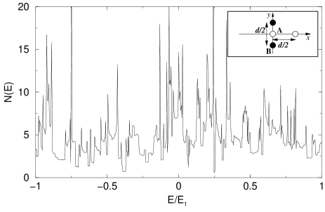
FIG. 7.: Band structure and density of states for a non-Bravais lattice with four vortices per unit cell with anisotropy ratio $\alpha_{D}=v_{F}/v_{\Delta}=5$. The position of the vortices in the unit cell is displayed in the inset, notice that there is no center of inversion symmetry and thus particle hole symmetry is absent.

Particle-hole symmetry requires a center of inversion in the unit cell to exist. We can break this symmetry considering a unit cell with a basis consisting of four vortices, so that its area is $2d^{2}$. We choose a rectangular unit cell with sides $-d<x<d$, $-d/2<y<d/2$. As an example, we can study the quasiparticle spectrum when the A-vortices are located at $(0,0)$ and $(d/2,0)$ and the B-vortices are located at $(0,\pm d/4)$, as shown in the inset in Fig. 7. In this case bands can go through the zero-energy axis away from crossings or near-crossings and thus the discussion in Section VIII doesn’t hold anymore and lines of zeroes can be found. The band structure in Fig. 7 for anisotropy $\alpha_{D}=5$ shows such lines of zero-energy states. Instead of going to zero, the density of states stays finite all the way down to zero energy, in close analogy to the prediction of the semiclassical theory [9]. It may also be seen that in this example, there is no particle-hole symmetry for the overall density of states for the exhibited band structure. We must recall, however, that the exhibited states are derived from only one of the four Dirac points, $\mbox{\boldmath$p$}=(0,p_{F})$, of the zero-field Fermi surface. If we include the contribution from the opposite point $\mbox{\boldmath$p$}=(0,-p_{F})$ the overall particle-hole symmetry will be recovered.

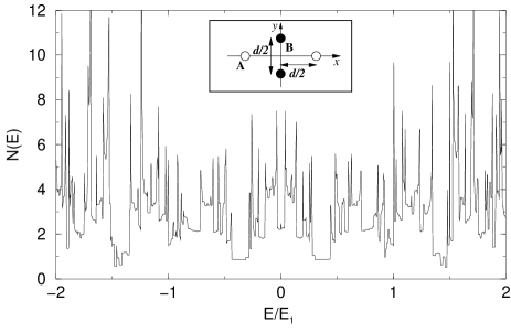
FIG. 8.: Band structure and density of states for a non-Bravais lattice with four vortices per unit cell with anisotropy ratio $\alpha_{D}=v_{F}/v_{\Delta}=5$. The position of the vortices in the unit cell is displayed in the inset, notice that there is a center of inversion symmetry with respect to which $\mbox{\boldmath$v$}^{A,B}(-\mbox{\boldmath$r$})=-\mbox{\boldmath$v$}^{A,B}(\mbox{\boldmath$r$})$. Particle-hole symmetry is preserved, although not independently at every point in the Brillouin zone: states at $k$ and $-\mbox{\boldmath$k$}$ have to be exchanged.

With four vortices per unit cell it is also possible to find superfluid velocity distributions that preserve particle-hole symmetry for the total density of states arising from a single Dirac point, but not at each point of the Brillouin zone separately as was the case for two vortices per unit cell. For example, the configuration depicted in Fig. 8, where the A-vortices are located at $(\pm d/2,0)$ while the B-vortices are at the same position as before, shows such a distribution. Here, if we consider the transformation $\mbox{\boldmath$r$}\to-\mbox{\boldmath$r$}$, the superfluid velocities $\mbox{\boldmath$v$}^{A}(\mbox{\boldmath$r$})$ and $\mbox{\boldmath$v$}^{B}(\mbox{\boldmath$r$})$ are not exchanged as in equation (29), rather they transform like $\mbox{\boldmath$v$}^{A,B}(-\mbox{\boldmath$r$})=-\mbox{\boldmath$v$}^{A,B}(\mbox{\boldmath$r$})$. The Hamiltonian (21) goes into minus itself if we take $\mbox{\boldmath$r$}\to-\mbox{\boldmath$r$}$ and simultaneously exchange $k$ with $-\mbox{\boldmath$k$}$. We then find $E_{+}(\mbox{\boldmath$k$})=-E_{-}(-\mbox{\boldmath$k$})$, but no particle-hole symmetry at a fixed $k$. The density of states is an even function of the quasiparticle energy, as can be observed in Fig. 8. Lines of energy-zeroes are still allowed in this case, so the density of states may be finite at $E=0$.

X Density of states: comparison with the semiclassical theory

The density of states is computed using a linear interpolation for the band structure in between the sampled $k-$points and is normalized as follows:

$$N(E)=2\sum_{n}\int\frac{d^{2}k}{(2\pi)^{2}}\delta(E-E_{n}(\mbox{\boldmath$k$}))$$ (73)

where the factor of 2 comes from spin degeneracy and $n$ is a band index. As we noted in the previous section, this is the contribution to the total density of states coming from one of the four nodes of the zero-field quasiparticle spectrum. For a simple square vortex lattice in the orientation we are considering, the total density of states can be obtained simply by multiplying this result by four. In more complicated vortex lattices, a separate calculation of the density of states at one of the nodes rotated by $90^{\circ}$ with respect to $\mbox{\boldmath$p$}=(0,p_{F})$ is generally necessary.

If the vortex lattice is a Bravais lattice, the quasiparticle spectra are gapless regardless of the anisotropy ratio $\alpha_{D}$ and the density of states at very low-energy is linear in energy although the slope is renormalized by the potentials (and the renormalization factor depends on $\alpha_{D}$). The results of the numerical diagonalization are shown in Figs. 3-5 for $\alpha_{D}=1,2,4$ respectively. The sharp peaks in the density of states are logarithmic van Hove singularities: for topological reasons every band in two dimensions has at least two saddle points which contribute logarithmically divergent peaks to the density of states. The van Hove singularities show up as finite-height peaks in the numerical evaluation of the density of states because of the linear interpolation scheme used for the band structure. Averaging these peaks out, however, one can see that at high energy the density of states reproduces the behavior expected for the quasiparticles in the absence of a magnetic field $N(E)=|E|/(\pi\hbar^{2}v_{F}v_{\Delta})$ as shown in Fig. 5 for the $\alpha_{D}=4$ case.

We want to compare our results to the semiclassical picture studied primarily by Volovik [9, 19]. This approach takes into account the superfluid velocity $\mbox{\boldmath$v$}_{s}$ distribution through the Doppler shift of the quasiparticle energy

$$E(\mbox{\boldmath$k$},\mbox{\boldmath$r$})=\pm\sqrt{\xi^{2}_{\mbox{\boldmath$\scriptstyle k$}}+\Delta_{d}(\mbox{\boldmath$k$})^{2}}+\hbar\mbox{\boldmath$k$}\cdot\mbox{\boldmath$v$}_{s}(\mbox{\boldmath$r$}),$$ (74)

where $\xi_{\mbox{\boldmath$\scriptstyle k$}}$ is the kinetic energy measured with respect to the Fermi surface. Within this framework Kopnin and Volovik introduced two crossover energy scales [19, 16, 20] $E_{1}\approx\hbar v_{F}/d$ and $E_{2}^{KV}\approx\hbar v_{\Delta}/d$. The first energy scale $E_{1}\approx\hbar v_{F}/d$ marks the boundary between the temperature dominated regime and the superflow dominated regime in the thermodynamic functions. Physically, this crossover corresponds to the WKB eigenfunctions becoming extended on a scale comparable to the intervortex distance, at least in one direction. For $E>E_{1}$, the states are unaffected by the magnetic field and the density of states is linear with the same slope one would find in the bulk without a vortex lattice, as we discussed in the previous paragraph. For $E<E_{1}$, the semiclassical density of states is essentially independent of energy [9] and for our order parameter distribution on a square lattice we calculate it to be

$$N(0)=\frac{1}{4\hbar v_{\Delta}d}.$$ (75)

Volovik finds essentially the same result [9], with an undetermined numerical prefactor which depends on the geometry of the vortex lattice. Won and Maki [28], using a somewhat different model, calculate this geometric prefactor for a general vortex lattice structure (although only Bravais lattices are considered) and find a result of the same order of magnitude of (75), for a square lattice.

The second crossover marks the boundary where a full quantum mechanical picture becomes important and the semiclassical analysis breaks down. We will call this scale $E_{2}$. As we mentioned above, Kopnin and Volovik [19, 16, 20] argue that this scale is linear in $1/\alpha_{D}$, and is given by $E_{2}^{KV}\approx\hbar v_{\Delta}/d$ and, for energies in the range $E_{2}^{KV}<E<E_{1}$, they predict a constant density of states. In terms of band structure this means that we need to find a direction in $k$-space in which the bands are flat on a scale of $E_{2}$. If we assume that the perturbation induced by the magnetic field is weak, and thus that the band structure is only weakly renormalized, we find that for large enough anisotropy $\alpha_{D}\gg 1$ several bands will start overlapping for energies $E<E_{1}$ and will have a small dispersion in the $k_{x}$ direction of the order of $\hbar v_{\Delta}/d$. The density of states for $E<E_{1}$ would then be essentially constant down to energies of the order of $\hbar v_{\Delta}/d$, which corresponds exactly to $E_{2}^{KV}$. For energies $E<E^{KV}_{2}$ we would have just a single band and the density of states would drop linearly to zero. The key assumptions that enter in this argument (weak perturbing potential) are essentially the absence of vanishing energies, or nearly vanishing energies, at any point in the Brillouin zone other than the $\Gamma$ point and a small renormalization of the slope of the lowest energy bands at the $\Gamma$ point in any direction of the Brillouin zone. These assumptions are satisfied for rather small anisotropy ratios $\alpha_{D}\ll 10$ but seem to fail for higher values of $\alpha_{D}$, as we will show.

In Fig. 3-5 we can see how the semiclassical description starts developing. For $\alpha_{D}=1$ there is no resemblance to the semiclassical behavior for any energy, the bands are very distinct at low energy and there is only one crossover from a quantum mechanical region to a purely classical region ($E>E_{1}$) without any hint of constant density of states. Changing the anisotropy to $\alpha_{D}=2$ or even better $\alpha_{D}=4$ a hint of the semiclassical region starts opening up and one can identify a trend towards a flat density of states between roughly $E_{2}^{KV}$ and $E_{1}$. For energies much lower than $E_{2}^{KV}$ the density of states is linear and goes to zero at zero energy. Although there is only one band (even in the $\alpha_{D}=4$ case) below $E_{1}$, the semiclassical description seems to start working remarkably well. From these plots we can already notice discrepancies with the Kopnin and Volovik picture. Notice that, while for the $\alpha_{D}=2$ case the ratio between the slopes in the $k_{y}$ and $k_{x}$ directions is $v_{F}^{R}/v_{\Delta}^{R}\approx 2.5\sim\alpha_{D}$ (the superscript $R$ indicates that these are the renormalized velocities in the two above mentioned directions in $k$-space), already in the $\alpha_{D}=4$ case the same ratio is roughly 17 which is much larger than $\alpha_{D}$. The scale at which the flat density of states should break down, $E_{2}$, seems to be much smaller than the simple argument above would predict.

FIG. 9.: Band structure for a square lattice with anisotropy ratio $\alpha_{D}=v_{F}/v_{\Delta}=$ 8, 12, 15 (solid, dashed and dot-dashed lines respectively) along the symmetry line $\Gamma$Y. Notice the apparent vanishing of the energy spectrum at a wavevector close to the Y point, for the large values of $\alpha_{D}$. (Our numerical calculation cannot distinguish between a true zero and a very small energy gap.) A second small energy gap is developing about one third of the way from $\Gamma$ to Y. Only the positive energy bands are plotted for clarity, the negative energy ones can be obtained by particle-hole symmetry. In the $\alpha_{D}=15$ only the two lowest bands are plotted, while all the bands with energy $E<\hbar v_{F}/d$ are plotted for $\alpha_{D}=$ 8, 12. The gaps at the $\Gamma$ point are fictitious and are due to the Wilson term in the Hamiltonian.

Besides a large renormalization of the slope of the energy bands at the $\Gamma$ point, which occurs even for relatively small anisotropies, we find for large anisotropies that there are lines in the Brillouin zone where the energy of the lowest band is very close to vanishing. As we discussed in Section VIII, we do not expect to find points, other than the $\Gamma$ point and possibly along the $k_{y}=0$ axis, where the energy is exactly zero (except, conceivably, at isolated values of the anisotropy ratio $\alpha_{D}$). For anisotropies $\alpha_{D}>8$ we cannot resolve numerically any dispersion along the $k_{x}$ direction, so only the $\Gamma$Y line of the band structure carries information. In Fig. 9 we have plotted a few of the lowest energy bands corresponding to values of the anisotropy ratio $\alpha_{D}=$8, 12, 15. One can immediately see one of these energy near-zeroes developing along the $\Gamma$Y axis. In general, the crossover scale $E_{2}$ will be set by the larger of the energy gap at this point and the energy dispersion in the $k_{x}$ direction. The density of states will be very close to a constant for energies larger than $E_{2}$ and will drop towards zero with decreasing energy for $E\ll E_{2}$. In this way the high-anisotropy limit approaches the semiclassical prediction much faster then linearly in $1/\alpha_{D}$. (The precise functional dependence of $E_{2}$ on $\alpha_{D}$ will be discussed in a later publication.)

For more complicated lattices, where there is not particle-hole symmetry at each point in the Brillouin zone, there is no argument to prevent zero crossings, and we do indeed find lines of zeroes for large values of $\alpha_{D}$ (see Figs. 7 and 8). Thus the density of states is finite at zero energy and the semiclassical results may apply down to zero energy.

XI Conclusions

In conclusion, we have studied the quasiparticle spectrum of a $d$-wave superconductor in the mixed state. One important step in solving the problem has been the transformation due to Franz and Tešanović [13] that maps the original Bogoliubov–de Gennes equation into a Dirac Hamiltonian in an effective periodic vector and scalar potential corresponding to zero average magnetic field. We have found both numerically and in perturbation theory that for a Bravais lattice of vortices the spectrum remains gapless when a magnetic field is turned on. We have showed that for vortex lattices which preserve the particle-hole symmetry of the energy spectrum there can only be other isolated Dirac points in the Brillouin zone and so they cannot change qualitatively the very low-energy density of states. Different conclusions are reached when more complicated vortex lattice structure (for example with four vortices per unit cell) are considered where lines of energy-zeroes can be found. In this case, the density of states is finite at zero energy for large enough anisotropy ratio $\alpha_{D}$. A non-Bravais vortex lattice with two-vortices per unit cell can break the symmetry that keeps the spectrum gapless and open gaps whose magnitude depends on both the magnitude and orientation of the distortion observable both in the numerics and perturbation theory, with good agreement between the two. Finally, the high-anisotropy limit has been investigated and it’s relation to the semiclassical analysis explained. The crossover scale between the semiclassical and quantum mechanical regime $E_{2}$ goes to zero for large values of the anisotropy much faster than linearly in $1/\alpha_{D}$, at least for the vortex lattice geometries considered here, and the density of states quickly approaches a constant value for energies $E_{2}<E<E_{1}$.

XII Acknowledgments

We are grateful for helpful discussions with Noam Bernstein and Greg Smith, and for support from NSF grant DMR 99-81283.

REFERENCES

- [1]
- [2] D. J. Van Harlingen, Rev. Mod. Phys. 67, 515 (1995).
- [3] B. Keimer, W. Y. Shih, R. W. Erwin, J. W. Lynn, R. Dogan, and I. A. Aksay, Phys. Rev. Lett. 73, 3459 (1994).
- [4] I. Maggio-Aprile, Ch. Renner, A. Erb, E. Walker, and Ø. Fischer, Phys. Rev. Lett. 75, 2754 (1995).
- [5] Ch. Renner, B. Revaz, K. Kadowaki, I. Maggio-Aprile, and Ø. Fischer, Phys. Rev. Lett. 80, 3606 (1998).
- [6] Philip Kim, Zhen Yao, Cristian A. Bolle, and Charles M. Lieber, cond-mat/9910184 (1999).
- [7] Yong Wang and A. H. MacDonald, Phys. Rev. B 52, R3876 (1995).
- [8] Kouji Yasui and Takafumi Kita, Phys. Rev. Lett. 83, 4168 (1999).
- [9] G. E. Volovik, JETP Lett. 58, 469 (1993).
- [10] L. P. Gor’kov and J. R. Schrieffer, Phys. Rev. Lett. 80, 3360 (1998).
- [11] P. W. Anderson, cond-mat/9812063 (1998).
- [12] A. S. Mel’nikov, J. Phys. Cond. Matt. 21, 4219 (1999).
- [13] M. Franz and Z. Tešanović, Phys. Rev. Lett. 84, 554 (2000).
- [14] May Chiao, P. Lambert, R. W. Hill, Christian Lupien, R. Gagnon, Louis Taillefer, and P. Fournier, cond-mat/9910367 (1999).
- [15] J. Mesot, M. R. Norman, H. Ding, M. Randeria, J. C. Campuzano, A. Paramekanti, H. M. Fretwell, A. Kaminski, T. Takeuchi, T. Yokoya, T. Sato, T. Takahashi, T. Mochiku, and K. Kadowaki, Phys. Rev. Lett. 83, 840 (1999).
- [16] G. E. Volovik, JETP Lett. 65, 491 (1997).
- [17] S. H. Simon and P. A. Lee, Phys. Rev. Lett. 78, 1548 (1997).
- [18] B. Revaz, J.-Y. Genoud, A. Junod, K. Neumaier, A. Erb, and E. Walker, Phys. Rev. Lett. 80, 3364 (1998).
- [19] N. B. Kopnin and G. E. Volovik, JETP Lett. 64, 690 (1996).
- [20] G. E. Volovik and N. B. Kopnin, Phys. Rev. Lett. 78, 5028 (1997).
- [21] May Chiao, R. W. Hill, Christian Lupien, Bojana Popić, Robert Gagnon, and Louis Taillefer, Phys. Rev. Lett. 82, 2943 (1999).
- [22] P. G. de Gennes, Superconductivity of Metals and Alloys (Addison-Wesley, Reading, MA, 1989).
- [23] D. L. Feder and C. Kallin, Phys. Rev. B 55, 559 (1997).
- [24] K. Chandrasekharan, Elliptic Functions (Springer-Verlag, Berlin, 1985).
- [25] D. C. Sorensen, in Parallel Numerical Algorithms, edited by D. E. Keyes, A. Sameh, and V. Venkatakrishnan (Kluwer, Dordrecht, 1995).
- [26] J. B. Kogut, Rev. Mod. Phys. 55, 775 (1983).
- [27] K. G. Wilson, in New Phenomena in Subnuclear Physics, edited by A. Zichichi (Plenum, New York, 1975), p. 13.
- [28] Hyekyung Won and Kazumi Maki, Phys. Rev. B 53, 5927 (1996).