Anisotropic Fermi Surfaces and Kohn-Luttinger Superconductivity in Two Dimensions

Abstract

The instabilities induced on a two-dimensional system of correlated electrons by the anisotropies of its Fermi line are analyzed on general grounds. Simple scaling arguments allow to predict the opening of a superconducting gap with a well-defined symmetry prescribed by the geometry of the Fermi line. The same arguments predict a critical dimension of 3/2 for the transition of the two-dimensional system to non-Fermi liquid behavior. The methods are applied to the $t-t^{\prime}$ Hubbard model in a wide range of dopings.

I Introduction

Two-dimensional electron systems are the stage in which most relevant quantum phase transitions arise. The prototype of these phenomena is the Mott-Hubbard transition[1], which can only be understood in the context of a very strong correlation between the electrons. Many of the properties of the high-$T_{c}$ superconductors are also supposed to be the consequence of strong correlations in the two-dimensional layers[2]. In both cases, these reflect themselves in the presence of very marked features in the single-particle dispersion relation. The case of the copper-oxide compounds has been actually studied with increasing accuracy from the experimental point of view, and the angle-resolved photoemission measurements have been able to characterize the drastic change that the dispersion relation suffers when the stechiometric material is increasingly doped[3]. In the antiferromagnetic insulator regime, the characteristic peaks at $(\pi/2,\pi/2)$ and symmetry related points are a consequence of the doubling of the unit cell and the hybridization of modes by the wavevector $(\pi,\pi)$[4]. In the superconducting regime, the two-dimensional layers tend to develop very flat bands at the points $(\pi,0)$ and $(0,\pi)$[3, 5]. It is not well-known the mechanism by which the electron system undergoes such an strong renormalization but, reversing the line of reasoning, one may ask to what extent the pronounced features of the Fermi surface are at the origin of the unconventional properties in the superconducting regime. More generally, there is a lack of some dynamical formulation predicting the evolution of the Fermi surface upon doping and, at this point, it is only possible to characterize the shapes that lead to the opening of a more stable phase (Mott insulator, superconductor).

In general, phases different from the normal metallic state may arise from instabilities that have their origin in the peculiar geometry of the Fermi surface. Such instabilities may lead in some instances to antiferromagnetism, superconductivity, or the formation of a charge-density-wave structure. A well-known example is the case of a Fermi surface with the property of nesting, that is, with two portions that are mapped one into the other by some fixed momentum ${\bf Q}$. The system shows then an enhanced response to a perturbation with such wavevector and, if the corresponding modulation is commensurate with the lattice, it may lead to antiferromagnetic order or to a charge-density-wave structure, depending on the character of the interaction[6]. On the other hand, there are also instances in which the geometry of the Fermi surface may give rise to a superconducting instability, starting from a pure repulsive interaction. The basis of this mechanism was laid down by Kohn and Luttinger back in 1965[7, 8, 9]. In the case of a 3D electron system with isotropic Fermi surface, there is an enhanced scattering at momentum transfer $2k_{F}$, which translates into a modulation of the effective interaction potential $V(r)\sim\cos(2k_{F}r)/r^{3}$. This oscillating behavior makes possible the existence of attractive channels, labelled by the angular momentum quantum number. The superconducting instability arises from the channel with the strongest attractive coupling. In two dimensions, however, it has been shown for the weakly non-ideal Fermi gas that the effective interaction vertex computed to second order in perturbation theory is independent of the momentum of particles at the Fermi surface[10]. In this case one has to invoke higher-order effects in the scattering amplitude in order to find any attractive channel[11]. Otherwise, superconductivity due to the Kohn-Luttinger mechanism also arises in 2D systems with a Fermi surface that deviates from perfect isotropy. It has been studied in the Hubbard model at very low fillings, for instance, with the result that the dominant instability may correspond to $d_{xy}$, $d_{x^{2}-y^{2}}$ or $p$-wave symmetry, depending on the next-to-nearest neighbor hopping[12, 13, 14].

In the present paper we review the possibility of Kohn-Luttinger superconductivity in the case of Fermi surfaces with a shape appropriate to the description of the two-dimensional hole-doped copper oxide layers. As we want to consider the regime around the optimum doping for superconductivity, this implies to deal with highly anisotropic Fermi surfaces. We recall that a most accurate description of the electronic interaction in the layers of the hole-doped cuprates is given by the Hubbard model with one-site repulsive interaction and significant next-to-nearest-neighbor hopping $t^{\prime}<0$[15]. The values that give the best fit to the Fermi lines determined by the photoemission experiments seem to be around $-0.3$ times the $t$ hopping parameter. Typical energy contour lines for that value are shown in Fig. 1. There we can appreciate how the topology of the Fermi line changes upon doping after passing through the saddle points at $(\pi,0)$ and $(0,\pi)$. Quite remarkably, for filling levels right below the Van Hove singularity the Fermi line develops inflection points, i.e. points at which the curvature changes sign. The presence of these points leads to a strong modulation of the effective interaction of particles at the Fermi line, as their scattering is enhanced at momentum transfer connecting every two opposite inflection points. This effect is reminiscent of what happens in the case of nesting of the Fermi surface, although in the present circumstance there are no finite portions of the Fermi line that are mapped by a given wavevector. As a consequence of that, there is not a marked tendency towards a magnetic instability, but the dominant instability corresponds to superconductivity by effect of the modulation along the Fermi line of the effective interaction between particles with opposite momentum[16].

FIG. 1.: Different shapes of the Fermi line for the $t-t^{\prime}$ Hubbard model about the Van Hove filling. Two opposite inflection points are marked on the figure.

We will see that, in the mentioned cases of strong anisotropy of the Fermi line, there is a direct correspondence between its topology and the channel in which the dominant superconducting instability opens up. As we will be carrying out the discussion for the $t-t^{\prime}$ Hubbard model, the channels are characterized by the irreducible representations of the discrete symmetry group. We will show that, in the case in which the Fermi line has a set of evenly distributed inflection points, superconductivity due to the Kohn-Luttinger mechanism takes place in the extendend $s$ channel, with nodes at the inflection points. On the other hand, when the Fermi line is above the saddle-points, the superconducting instability most likely takes place in the $d_{x^{2}-y^{2}}$ channel, with nodes at the points where the curvature reaches a minimum. Between these two instances, we find the situation in which the Fermi energy sits at the Van Hove singularity, what requires special care in order to deal with the divergences that appear in perturbation theory associated to the logarithmic density of states. In the context of highly anisotropic Fermi surfaces, the implementation of the Kohn-Luttinger mechanism was proposed within the investigation of the electron system near Van Hove singularities[17]. Related analyses have been also undertaken by other authors[18, 19, 20]. As we will see, such an electronic mechanism of superconductivity near a Van Hove singularity may be relevant to the physics of the high-$T_{c}$ cuprates[21, 22, 23]. From the technical point of view, this is due to the fact that the modulation of the effective interaction vertex is driven then by a marginal operator, rather than by an irrelevant operator as it happens in general, so that in some region of the phase diagram critical temperatures may be reached as high as those found in the cuprates[24].

We will adopt a renormalization group (RG) approach to the discussion of the subject. In recent years, RG methods have been applied to the description of interacting electron systems[6, 25]. They have given a precise characterization of Fermi liquid theory, as well as an efficient classification of its relevant perturbations[6]. Among a reduced number of them, superconductivity appears as one of the possible instabilities. It only requires the presence of an attractive coupling in some channel, though small it may be in the bare theory. RG methods are also particularly well-suited to the discussion of highly anisotropic Fermi surfaces, since a change of the topology is accompanied by a change of the scaling dimension of the interaction vertex. This is the way in which the enhancement of scattering produced by some features, as for instance the inflection points, is understood in the RG framework[16]. The RG approach is specially useful when dealing with unconventional mechanisms of superconductivity, as it may face the possibility that the normal state does not fall into the Fermi liquid description. Under this circumstance, it may not be justified to use a perturbative approach, or even to rely on certain sum of diagrams in perturbation theory, to study the superconducting instability. Yet in the RG approach the only basic assumption is that there is a well-defined scaling near the Fermi level, which allows to identify the scaling operators in the low-energy effective theory. Apart from addressing the question of superconductivity, the discussion can be devoted to establish when such scaling conveys to non-Fermi liquid behavior[26], spoiling the conventional picture that considers superconductivity as a low-energy instability of Fermi liquid theory.

The paper is organized as follows. In the next section we briefly review the renormalization group approach to interacting electron systems. In section 3 we investigate under which conditions non-Fermi liquid behavior may arise by effect of the anisotropy of the Fermi surface. The analysis of the superconducting instabilities in the presence of inflection points in the Fermi line is carried out in section 4. The RG approach is adapted to the discussion of the 2D electron system near Van Hove singularities in section 5. Finally, our conclusions and outlook are drawn in section 6.

II Renormalization Group Approach to Interacting Electrons

The wilsonian RG approach, that has proven to be so useful in the study of classical statistical systems, has been recently implemented in the investigation of many-body systems with a Fermi surface[6]. In this context, the basic idea of the method is closely related to the concept of effective field theory[25]. One is interested in identifying the elementary fields and excitations at a very low energy scale about the Fermi level, that is, at a much smaller scale than the typical electron energies of the bare theory. The strategy to accomplish this task is to perform a progressive integration of high-energy modes living in two thin shells at distance $\Lambda$ in energy below and above the Fermi surface. Sufficiently close to it, the fields of the effective theory have to scale appropriately under a reduction of the cutoff $\Lambda\rightarrow s\Lambda$. Then, one can make an inspection of all the possible terms built out of them contributing to the effective action of the theory, checking their behavior under the scale transformation

$$g_{i}\;\int dtd^{D}p\;{\cal O}_{i}\rightarrow g_{i}\;s^{\alpha_{i}}\;\int dtd^{D}p\;{\cal O}_{i}$$ (1)

The terms in the effective action that scale with an exponent $\alpha_{i}>0$ are said to be irrelevant, as their effect becomes weaker and weaker close to the Fermi surface. On the other hand, if there appear some terms scaling with $\alpha_{i}<0$, this means that we have chosen a wrong starting point for the effective field theory, since there are couplings that are not stabilized already at the classical level. The interesting case corresponds to having all the exponents $\alpha_{i}\geq 0$ and, in particular, operators with $\alpha_{i}=0$ (so called marginal operators), as this is the situation where the RG approach can address the existence of a fixed-point of the scale transformations in the low-energy theory.

The system of interacting electrons with a sphere-like Fermi surface provides a good example of how the above program is at work[27]. We focus from now on in two spatial dimensions and write the action with the most general four-fermion interaction term

$$S = \int dtd^{2}p\left(i\Psi^{+}_{\sigma}({\bf p})\partial_{t}\Psi_{\sigma}({\bf p})-\left(\varepsilon({\bf p})-\varepsilon_{F}\right)\Psi^{+}_{\sigma}({\bf p})\Psi_{\sigma}({\bf p})\right)$$ (3)

$$+\int dtd^{2}p_{1}d^{2}p_{2}d^{2}p_{3}d^{2}p_{4}\;U({\bf p}_{1},{\bf p}_{2},{\bf p}_{3},{\bf p}_{4})\;\Psi^{+}_{\sigma}({\bf p}_{1})\Psi^{+}_{\sigma^{\prime}}({\bf p}_{2})\Psi_{\sigma^{\prime}}({\bf p}_{4})\Psi_{\sigma}({\bf p}_{3})\delta({\bf p}_{1}+{\bf p}_{2}-{\bf p}_{3}-{\bf p}_{4})$$

We suppose that the integration of high-energy modes has already proceed to energies close to the Fermi level, so that $\Psi({\bf p})$ stands here for some renormalized scaling fermion field. The important point to notice is that, at each point of the Fermi line, only the component of the momentum orthogonal to it scales with the energy cutoff. In fact, near the Fermi level we can decompose every momentum ${\bf p}$ into a vector ${\bf P}$ to the closest point in the Fermi line and the orthogonal component ${\bf p}_{\perp}$, as shown in Fig. 2,

$${\bf p}={\bf P}+{\bf p}_{\perp}$$ (4)

Upon the scale reduction of the energy cutoff, we have ${\bf p}_{\perp}\rightarrow s{\bf p}_{\perp}$.

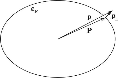
FIG. 2.: Decomposition of the momentum ${\bf p}$ into a transverse and a large component at the Fermi line.

It becomes clear, for instance, that in the noninteracting theory the field $\Psi({\bf p})$ has a well-defined scaling rule that makes the first term of (3) scale invariant. We can rewrite the free effective action in the form

$$S_{0}\sim\int dtdPdp_{\perp}\left(i\Psi^{+}_{\sigma}({\bf p})\partial_{t}\Psi_{\sigma}({\bf p})-v_{F}({\bf P})p_{\perp}\Psi^{+}_{\sigma}({\bf p})\Psi_{\sigma}({\bf p})\right)$$ (5)

Under a change of the cutoff $\Lambda\rightarrow s\Lambda$ and corresponding changes in the scaling variables $t\rightarrow s^{-1}t,p_{\perp}\rightarrow sp_{\perp}$, the field has to transform according to $\Psi({\bf p})\rightarrow s^{-1/2}\Psi({\bf p})$ in order to keep (5) marginal.

A similar analysis applied to the interaction term of the effective action

$$S_{int} \sim \int dtdP_{1}dp_{1\perp}dP_{2}dp_{2\perp}dP_{3}dp_{3\perp}dP_{4}dp_{4\perp}$$ (7)

$$U({\bf p}_{1},{\bf p}_{2},{\bf p}_{3},{\bf p}_{4})\;\Psi^{+}_{\sigma}({\bf p}_{1})\Psi^{+}_{\sigma^{\prime}}({\bf p}_{2})\Psi_{\sigma^{\prime}}({\bf p}_{4})\Psi_{\sigma}({\bf p}_{3})\delta({\bf p}_{1}+{\bf p}_{2}-{\bf p}_{3}-{\bf p}_{4})$$

leads to the conclusion that, in general, it scales in the form $S_{int}\rightarrow sS_{int}$. We are assuming that, upon scaling, the orthogonal component of the momenta are irrelevant in the momentum-conservation delta function, compared to the large ${\bf P}$ components, so that $\delta({\bf p}_{1}+{\bf p}_{2}-{\bf p}_{3}-{\bf p}_{4})\approx\delta({\bf P}_{1}+{\bf P}_{2}-{\bf P}_{3}-{\bf P}_{4})$. Thus the interaction turns out to be irrelevant for generic values of the momenta (assuming implicitly a smooth dependence on them of the potential $U({\bf p}_{1},{\bf p}_{2},{\bf p}_{3},{\bf p}_{4})$).

The important remark put forward in Refs. [6] and [25] is that there are special processes in which the kinematics forces a different scaling behavior through the constraint of momentum conservation. This is the case when the combination of the momenta at the Fermi surface identically vanishes, ${\bf P}_{1}+{\bf P}_{2}-{\bf P}_{3}-{\bf P}_{4}=0$. When this happens, the scaling of the orthogonal components of the momenta is transferred to the scaling of the delta function, and the four-fermion interaction term becomes marginal. This explains why in Fermi liquid theory there are only a few channels that are not irrelevant in the low-energy theory.

Specifically, the above identity for the sum of the components at the Fermi surface is satisfied by i) ${\bf P}_{1}=-{\bf P}_{2}$ and ${\bf P}_{3}=-{\bf P}_{4}$, what characterizes the so called BCS channel, ii) ${\bf P}_{1}={\bf P}_{3}$ and ${\bf P}_{2}={\bf P}_{4}$, that leads to the forward scattering channel, and iii) ${\bf P}_{1}={\bf P}_{4}$ and ${\bf P}_{2}={\bf P}_{3}$, that differs from the previous one by the exchange of the outgoing particles. In this classification we have not taken into account the spin of the particles, but it is clear that, if in the third case the spin of ${\bf P}_{4}$ is different to that of ${\bf P}_{1}$, the scattering process is fully differenciated from that of forward scattering. In the case of a spin-dependent interaction, it makes sense to consider iii) as a different channel on its own, that we will call exchange scattering channel[28]. The three different channels leading to marginal interactions are represented graphically in Fig. 3.

FIG. 3.: Marginal interactions in Fermi liquid theory.

We address now the behavior of the marginal interactions under quantum corrections by focusing again on a system with a Fermi line having the topology of the circle. This is actually the case best studied in the literature. We borrow the main conclusions from Refs. [6] and [25], which state, to begin with, that the interaction in the forward scattering channel remains unrenormalized in the quantum theory. That is, the integration of the high-energy modes does not produce any dependence of such marginal interaction on the cutoff by effect of the loop corrections. This is the way in which the Landau theory of the Fermi liquid is recovered in the present context, with a finite correction of the bare parameters and a $F$ function that encodes all the information about the four-fermion interaction.

On the other hand, the pairing interaction in the BCS channel gets dependence on the cutoff by integration of modes in the two thin slices at energies $\Lambda$ and $-\Lambda$. At the one-loop level, for instance, the particle-particle bubble is the diagram that contributes to the renormalization since, if one of the particles in the loop carries momentum ${\bf p}$ at the slice being integrated, the other has a momentum $-{\bf p}$ that also belongs to the slice. In two dimensions, taking into account the dependence of the BCS coupling on the angles $\theta$ and $\theta^{\prime}$ of the respective incoming and outgoing pairs, the one-loop differential correction becomes

$$V_{\Lambda+d\Lambda}(\theta,\theta^{\prime})\approx V_{\Lambda}(\theta,\theta^{\prime})+N(\varepsilon_{F})\;d\Lambda\;\int d\theta^{\prime\prime}V_{\Lambda}(\theta,\theta^{\prime\prime})V_{\Lambda}(\theta^{\prime\prime},\theta^{\prime})\;\;\;\;,\;\;\;\;d\Lambda<0$$ (8)

where $N(\varepsilon_{F})$ is the density of states at the Fermi level.

The one-loop flow equation

$$\Lambda\frac{\partial V(\theta,\theta^{\prime})}{\partial\Lambda}=N(\varepsilon_{F})\int d\theta^{\prime\prime}V(\theta,\theta^{\prime\prime})V(\theta^{\prime\prime},\theta^{\prime})$$ (9)

describes the approach to the Fermi line as $\Lambda\rightarrow 0$. Thus, in systems where the original bare interaction is repulsive the BCS channel has a general tendency to become suppressed at low energies. It is only when $V$ or any of its normal modes is negative that the renormalized coupling becomes increasingly attractive near the Fermi level. This is the way in which the superconducting instability arises in the RG framework[6, 25]. The main conclusion is that the system with uniform repulsive interaction and isotropic Fermi line provides a paradigm of the Landau theory of the Fermi liquid, since all the interactions turn out to be irrelevant but the $F$ interaction, that remains finite and non-zero close to the Fermi level.

The above RG scheme gives also the clue of why the slight deviation from isotropy may trigger the onset of superconductivity. In general the analysis has to be carried over the couplings $V_{n}$ for the normal modes appropriate to the symmetry of the Fermi line. The flow equation may be decomposed then into

$$\Lambda\frac{\partial V_{n}}{\partial\Lambda}=N(\varepsilon_{F})V^{2}_{n}$$ (10)

and the flow of the couplings is given by

$$V_{n}(\Lambda)=\frac{V_{n}(\Lambda_{0})}{1+N(\varepsilon_{F})\;V_{n}(\Lambda_{0})\;\log(\Lambda_{0}/\Lambda)}$$ (11)

If, at some intermediate scale $\Lambda_{0}$, a coupling $V_{n}(\Lambda_{0})$ becomes negative, then a superconducting instability develops in the corresponding mode. The Kohn-Luttinger mechanism is based on the fact that this happens in practice, even for an isotropic Fermi surface in three dimensions, since the corrections to the bare $V(\theta,\theta^{\prime})$ by particle-hole diagrams already introduce the degree of anisotropy needed to turn some of the $V_{n}$ negative[7]. In two dimensions, the anisotropy of the Fermi line is also a necessary condition to produce an attractive interaction in some of the normal modes, as pointed out in Ref. [10], unless the particle-hole corrections to the bare $V(\theta,\theta^{\prime})$ are carried out beyond second order in perturbation theory[11].

Previous analyses of the Kohn-Luttinger mechanism have focused on small deviations from isotropy of the Fermi line[8]. The relevance of the superconducting transition is related anyhow to the source of anisotropy that is producing the attractive coupling in the model. An attractive but very tiny $V_{n}(\Lambda_{0})$ may lead to superconductivity at a very small scale $E\sim\Lambda_{0}\exp\{1/\left(N(\varepsilon_{F})V_{n}(\Lambda_{0})\right)\}$. Our RG analysis makes clear that the anisotropy has an effect through corrections to the bare scattering $V(\theta,\theta^{\prime})$ that are irrelevant as the cutoff $\Lambda\rightarrow 0$. We will see that they scale in general like $\Lambda^{1/2}$, that is, with the same scaling law as for scattering with $2k_{F}$ momentum transfer in the isotropic Fermi line. On the other hand, we will be dealing with topological features of the Fermi line, i.e. inflection points, that enhance the attractive modes to scale like $\Lambda^{1/4}$[16]. Inflection points can be thought of as precursors of the development of the saddle points at the Fermi line, a situation in which the particle-hole corrections to scattering processes become marginal ($\sim\Lambda^{0}$ ). Consequently, in the context we are facing of a repulsive bare interaction, the superconducting instability is significantly strengthened near the Van Hove singularity[17, 18, 19, 20, 29], although then there is also competition with magnetic instabilities in the system[23, 30, 31, 32, 24]. The RG analysis of the problem becomes quite delicate, moreover, as one has to derive a proper scaling in a model which has enhanced $\log^{2}(\Lambda)$ divergences in the BCS channel. The special topology of the Fermi line passing by the saddle points introduces significant changes in the analysis carried out for the Fermi liquid theory and it requires the specific treatment that we will discuss in Section 5.

III Inflection points of the Fermi line

As discussed in the preceding section, the scaling of the different couplings can be read off from the cutoff dependence of the particle-particle and particle-hole diagrams which modify them. When the cutoff is sufficiently close to the Fermi surface, these diagrams are reduced to convolutions of single particle propagators taken at the Fermi surface. The relevance or irrelavance of the couplings is determined by the density of states of electron hole pairs, or of two electron states.

We can deduce the real part of a given diagram from its imaginary part by performing a Hilbert transform. The imaginary parts measure directly the density of excited states, and are usually easier to estimate. Let us now imagine that we can determine that, for a given susceptibility, $\chi$, the low energy behavior is ${\rm Im}\chi({\bf q},\omega)\sim\omega^{\alpha}$. Then, ${\rm Re}\chi({\bf q},\omega)$ includes a term with the same $\omega$ dependence if $\alpha\neq 0$, and shows a logarithmic behavior if $\alpha=0$. This contribution will dominate the corrections to the couplings when it is present.

The quantity ${\rm Im}\chi({\bf q},\omega)$ is a measure of the electron-hole or electron-electron excitations of total momentum ${\bf q}$ and energy $\omega$. The simplest way to estimate it is to measure the total number of excitations with momentum ${\bf q}$ and energy equal or less than $\omega$. By deriving the volume of phase space which fulfills these contraints with respect to $\omega$, one obtains ${\rm Im}\chi({\bf q},\omega)$.

The leading diagram which has a non trivial low energy behavior is the electron electron propagator at zero momentum, the BCS channel, as discussed in the previous section. It is easy to show that ${\rm Im}\chi_{BCS}({\bf q}\rightarrow 0,\omega)\rightarrow$ constant as $\omega\rightarrow 0$. This diagram describes the main instability of Fermi liquids. In the following, we analyze the modifications that insertions of electron-hole propagators induce in this channel, following the ideas of Kohn and Luttinger.

We first need to estimate the the energy dependence of the electron hole propagator ${\rm Im}\chi({\bf q},\omega)$. In one dimension, it is relatively straightforward to show that the imaginary part of the electron-hole susceptibility, ${\rm Im}\chi(q,\omega)$, is finite all the way to zero energy only when $q=2k_{F}$. The limit of ${\rm Im}\chi(2k_{F},\omega)$ as $\omega\rightarrow 0$ goes as the single particle density of states at the Fermi level (a schematic view of the available density of states is shown in Fig. 4 ).

From $\lim_{\omega\rightarrow 0}{\rm Im}\chi(2k_{F},\omega)\propto{\rm Im}G(\varepsilon_{F})$, we deduce that $\lim_{\omega\rightarrow 0}{\rm Re}\chi(2k_{F},\omega)\propto{\rm Im}G(\varepsilon_{F})\log(\Lambda/\omega)$, where $\Lambda$ is the cutoff of the theory. Outside $q=2k_{F}$ there are no gapless electron-hole excitations in one dimension. The log dependence in ${\rm Re}\chi$, when inserted in the appropiate diagrams, leads to the existence of marginal couplings, and to the non trivial phenomenology of Luttinger liquids.

In higher dimensions, ${\rm Im}\chi({\bf q},\omega)$ remains finite at low energies when ${\bf q}$ connects two points at the Fermi surface. The density of electron-hole pairs at this wavevector depends on the curvature of the Fermi surface at these two points, and also on their relative orientation. In general, the two patches of the Fermi surface are not parallel. We can linearize the dispersion relation as $\varepsilon({\bf k}_{i}+{\bf k}^{\prime})={\bf v}_{F}^{i}{\bf k}^{\prime}$, where ${\bf k}_{1}={\bf k}_{0}$ and ${\bf k}_{2}={\bf k}_{0}+{\bf q}$ denote two points at the Fermi surface. The constraints described earlier imply that: $\omega\geq\varepsilon({\bf k}_{1}+{\bf k}^{\prime})-\varepsilon({\bf k}_{2}+{\bf k}^{\prime})$, and, simultaneously, $\varepsilon({\bf k}_{1}+{\bf k}^{\prime})>0$ and $\varepsilon({\bf k}_{2}+{\bf k}^{\prime})<0$. These three conditions, if ${\bf v}_{F}^{1}$ and ${\bf v}_{F}^{2}$ are not parallel, define a triangle in ${\bf k}^{\prime}$ space such that the basis and the height are proportional to $\omega$, as schematically shown in Fig. 5. Thus, ${\rm Im}\chi({\bf q},\omega)\propto\omega$. This linear dependence on $\omega$ remains when the local density of electron-hole excitations is determined, by integrating over ${\bf q}$. This is the relevant quantity which determines the coupling of impurities to the electron liquid, and can lead to non trivial divergences in perturbation theory, as best shown in the Kondo model.

The previous analysis does not hold when ${\bf q}$ connects two regions of the Brillouin Zone where the Fermi surface is parallel. The simplest case is also shown in Fig. 5. The linear expansion of the dispersion relation is not enough to estimate ${\rm Im}\chi$. Using a frame of reference such that one axis is perpendicular to the two Fermi surfaces, one can write:

$$\varepsilon({\bf k}_{1}+{\bf k}^{\prime}) = v_{F}^{1}k^{\prime}_{\perp}+\alpha_{1}k^{\prime 2}_{\parallel}$$ (12)

$$\varepsilon({\bf k}_{2}+{\bf k}^{\prime}) = v_{F}^{2}k^{\prime}_{\perp}+\alpha_{2}k^{\prime 2}_{\parallel}$$ (13)

The boundaries in ${\bf k}^{\prime}$ of the region where particle-hole excitations of energy less than $\omega$ are possible are given by $k^{\prime}_{\perp}\sim\omega/(v_{F}^{1}+v_{F}^{2})$ and $k^{\prime}_{\parallel}\sim\sqrt{\omega/(\alpha_{1}+\alpha_{2})}$, giving a total area $\propto\omega^{3/2}$. Hence, ${\rm Im}\chi({\bf q},\omega)\sim\sqrt{\omega}$. This analysis is restricted to two spatial dimensions. In higher dimensions, one has to take into account the additional $D-2$ dimensions. Along each of them, the available area is limited to a vector in $k$ space which also scales as $\sqrt{\omega}$. Hence, the volume is $\propto\omega^{(D+1)/2}$, and ${\rm Im}\chi({\bf q},\omega)\sim\omega^{(D-1)/2}$. There is a logarithmic divergence in ${\rm Re}\chi$ when $D=1$, which plays the role of the upper critical dimension.

We now assume that the Fermi surface is sufficiently anisotropic, as shown in Fig. 6, so that there are inflections points at wavevectors $\{{\bf k}_{i}\}$. A momentum transfer equal to ${\bf q}_{i}=2{\bf k}_{i}$ connects the two inflection points at $\pm{\bf k}_{i}$ which, in addition, define parallel patches of the Fermi surface. The expansion in Eq. (13) is not enough, as $\alpha_{1}=\alpha_{2}=0$. It must be replaced by:

$$\varepsilon({\bf k}_{1}+{\bf k}^{\prime}) = v_{F}k^{\prime}_{\perp}+\beta k^{\prime 3}_{\parallel}+\gamma k^{\prime 4}_{\parallel}$$ (14)

$$\varepsilon({\bf k}_{2}+{\bf k}^{\prime}) = -v_{F}k^{\prime}_{\perp}-\beta k^{\prime 3}_{\parallel}+\gamma k^{\prime 4}_{\parallel}$$ (15)

where we are using the symmetry between the two points. The area with electron-hole pairs with energy equal or less than $\omega$ is now limited by $k^{\prime}_{\perp}\sim\omega/v_{F}$ and $k^{\prime}_{\parallel}\sim(\omega/\gamma)^{1/4}$. Hence, ${\rm Im}\chi({\bf q},\omega)\sim\omega^{1/4}$.

The previous argument can be extended to arbitrary dimensions. In general, an inflection point along one of the $D-1$ transverse directions at the Fermi surface will not coincide with an inflection point along another direction. Thus, in the remaining $D-2$ directions, the phase space is limited by quadratic terms, obtained from an expansion like that in Eq. (13). Hence, ${\rm Im}\chi({\bf q},\omega)\sim\omega^{(D-2)/2+1/4}$. The dependence of ${\rm Re}\chi$ on the high energy cutoff of the theory becomes logarithmic when $D=3/2$ [16]. In the RG language, the couplings at wavevector ${\bf q}$ are marginal, and require a non trivial renormalization, at this dimension. It is interesting to note that, for isotropic Fermi surfaces, the critical dimension is 1[33, 34].

IV Anisotropic Fermi lines and Kohn-Luttinger superconductivity

In the previous Section we have seen that the strength of electron scattering bears a direct relation with the curvature at each point of the Fermi line. When this becomes highly anisotropic, the strong modulation in the angular dependence of the scattering between particles with momentum ${\bf p}$ and ${\bf-p}$ may lead to a superconducting instability, as explained in Section 2. We will address here the effect of inflection points in the $t-t^{\prime}$ Hubbard model, that is the simplest model with this kind of features in the Fermi line, and we will determine the symmetry channels in which pairing can take place.

The main issue is whether there exists any attractive coupling, at some intermediate energy scale $\Lambda_{0}$, for some of the normal modes of the bare BCS vertex $V(\Lambda_{0})$. Here $\Lambda_{0}$ is supposed to be a small fraction of the whole bandwidth, but not yet at the final stage of the renormalization process. We recall that $V$ depends on the angles $\theta$ and $\theta^{\prime}$ of the respective incoming and outgoing pairs of electrons, so that it may be decomposed into eigenfunctions with well-defined transformation properties under the action of the lattice symmetry group $D_{4}$. This has four one-dimensional representations, labelled respectively by $A_{1},A_{2},B_{1}$ and $B_{2}$, and a two-dimensional representation labelled by $E$. The complete sets of eigenfunctions for the respective irreducible representations are given by

$$A_{1} : \left\{\cos(4n\theta),n\in\rm{\bf N}\right\}$$ (16)

$$A_{2} : \left\{\sin(4n\theta),n\in\rm{\bf N}\right\}$$ (17)

$$B_{1} : \left\{\cos\left((4n+2)\theta\right),n\in\rm{\bf N}\right\}$$ (18)

$$B_{2} : \left\{\sin\left((4n+2)\theta\right),n\in\rm{\bf N}\right\}$$ (19)

$$E : \left\{a\sin\left((2n+1)\theta\right)+b\cos\left((2n+1)\theta\right),n\in\rm{\bf N}\right\}$$ (20)

Thus, the BCS vertex may be expanded in the form

$$V(\theta,\theta^{\prime}) = V_{0}+V_{1}\left(\cos(\theta)\cos(\theta^{\prime})+\sin(\theta)\sin(\theta^{\prime})\right)+V_{2}\cos(2\theta)\cos(2\theta^{\prime})+V_{3}\sin(2\theta)\sin(2\theta^{\prime})$$ (22)

$$+V_{4}\left(\cos(3\theta)\cos(3\theta^{\prime})+\sin(3\theta)\sin(3\theta^{\prime})\right)+V_{5}\cos(4\theta)\cos(4\theta^{\prime})+V_{6}\sin(4\theta)\sin(4\theta^{\prime})+\ldots$$

According to the discussion in Section 2, it suffices that any of the $V_{n}$ couplings becomes negative for a superconducting instability to take place in the process of renormalization, with the corresponding symmetry of the order parameter —$s$-wave in the case of $A_{1}$ and $A_{2}$, and $d$-wave in the case of the $B_{1}$ and $B_{2}$ representations.

We know that all the interactions are irrelevant in Fermi liquid theory, except the marginal $V$, $F$ and $E$ interactions. Furthermore, a repulsive interaction in the $V$ channel flows to zero upon renormalization towards the Fermi level. The point is that, even starting with a bare repulsive interaction as in the $t-t^{\prime}$ Hubbard model, some of the irrelevant couplings may lead to attraction in the BCS channel well before arriving at the final stage of the renormalization process. Under these circumstances, one needs to make an inspection of the theory at the intermediate scale $\Lambda_{0}$, in which the irrelevant interactions discussed in Section 2 have not become negligible yet. They may turn negative, in fact, some of the $V_{n}$ couplings. When this happens, by considering $\Lambda_{0}$ as the starting point of the renormalization group flow one observes the appearance of a strong attraction that leads to superconductivity in the low-energy effective theory.

Before switching on the quantum corrections, the marginal interaction $V$ equals the bare on-site repulsion $U$ of the $t-t^{\prime}$ Hubbard model. Given that the corrections we want to study at the intermediate scale $\Lambda_{0}$ are given by irrelevant operators, we may estimate their effect in perturbation theory. At the one-loop order, the diagrams that contribute in general are those in Fig. 7. In the case of the local Hubbard interaction, we take the convention of writing it as mediated by a potential between currents of opposite spin. This makes clear that the first two diagrams in Fig. 7 cannot be drawn with the interaction at hand, since they require an interaction between currents with parallel spins. They are present in the case of more general short-range interactions, but they tend to cancel out when such range shrinks to zero.

The contribution $\Pi(\theta,\theta^{\prime})$ of diagram $(c)$ has the overall effect of reinforcing the bare repulsion between the electrons. We recall that $\theta$ and $\theta^{\prime}$ label the angles between the incoming momentum ${\bf p}$ and the outgoing momentum ${\bf k}$, respectively, and the $x$ axis. When the two angles are the same, the momentum flowing in the interactions is large and connects opposite points at the Fermi line. We may borrow then the results of the previous Section to determine the scaling of the particle-hole contribution $\Pi(\theta,\theta)$ correcting $V(\theta,\theta)$.

The simplest case to discuss is that of a set of eight inflection points on the Fermi line evenly distributed in the angular variable $\theta$. Then the function $\Pi(\theta,\theta)$ must admit an approximate representation of the form

$$\Pi(\theta,\theta)\approx a+b\sin^{2}(4\theta)$$ (23)

We know from the previous Section that the coefficients $a$ and $b$ have different order of magnitude, given their different dependence on the energy cutoff $\Lambda_{0}$. At $\theta=0$, the scattering does not differ much from that of momentum transfer $2k_{F}$ on an isotropic Fermi line, so that $a\sim O(\Lambda_{0}^{1/2}/\alpha^{1/2})$, with the notation of the previous Section. At $\theta=\pi/8$, the scattering is greatly enhanced since it takes place between particles sitting at opposite inflection points on the Fermi line, implying $b\sim O(\Lambda_{0}^{1/4}/\gamma^{1/4})$.

The approximate expression for the bare BCS vertex at the energy scale $\Lambda_{0}$

$$U+\Pi(\theta,\theta)\approx U+a+b\sin^{2}(4\theta)$$ (24)

matches well the expansion (22) truncated to include up to the $V_{6}$ term. This allows to find the scaling of some combinations of the coefficients

$$V_{0}+V_{1}+V_{2}+V_{4}+V_{5}-U \sim O(\Lambda_{0}^{1/2})$$ (25)

$$V_{3}-V_{2} \sim 0$$ (26)

$$V_{6}-V_{5} \sim O(\Lambda_{0}^{1/4})$$ (27)

In order to close this system of equations we need an additional piece of information, that we get by estimating $\Pi(\theta,-\theta)$. This object stands for the scattering with a momentum transfer connecting a point on the Fermi line and its symmetric with respect to the $y$ axis. Therefore, it has again the characteristic dependence $\sim O(\Lambda_{0}^{1/2}/\alpha^{1/2})$ if $\theta=0$ or $\pi$ and it shows a crossover to a behavior $\sim O(\Lambda_{0})$ for other values of $\theta$. We may approximate then $\Pi(\theta,-\theta)\approx c+d\cos^{2}(\theta)$, where $c\sim O(\Lambda_{0})$ and $d\sim O(\Lambda_{0}^{1/2})$. Comparing with (22), this implies that

$$V_{0}-V_{1}-V_{3}-V_{4}-V_{6}-U \sim O(\Lambda_{0})$$ (28)

$$2V_{1} \sim O(\Lambda_{0}^{1/2})$$ (29)

$$V_{2}+V_{3} \sim 0$$ (30)

$$V_{4} \sim 0$$ (31)

$$V_{5}+V_{6} \sim 0$$ (32)

Putting together (27) and (32), we obtain $V_{6}\sim-V_{5}\sim O(\Lambda_{0}^{1/4})$, $V_{0}-U\sim O(\Lambda_{0}^{1/4})$ and $V_{1}\sim O(\Lambda_{0}^{1/2})$, the rest of the coefficients being higher-order powers of $\Lambda_{0}^{1/4}$.

Our analysis shows that there is a negative coupling at an intermediate energy scale $\Lambda_{0}$ in the expansion in normal modes of the marginal interaction $V(\theta,\theta^{\prime})$. The negative coupling $V_{5}$ sets actually the leading behavior of the coefficients $V_{n}$, for $n\neq 0$, as the energy cutoff is sent to the Fermi level. The approximations we have made of $\Pi(\theta,\theta)$ and $\Pi(\theta,-\theta)$ by specific periodic functions do not have therefore major influence in the determination of the attractive channel, as long as the higher harmonics in the expression (22) can be considered subdominant with respect to the behavior of the couplings $V_{1}$, $V_{5}$ and $V_{6}$.

We conclude that there must be a range of dopings, around the filling level where the inflection points are evenly distributed in the angular variable on the Fermi line, in which a superconducting instability opens up in the channel corresponding to the $A_{1}$ representation of the lattice symmetry group[16]. This means that the order parameter of superconductivity has the so-called extended $s$-wave symmetry, with nodes at the inflection points of the Fermi line. This location of the nodes has to be shared to a certain degree of approximation by any Fermi line with a set of inflection points. The gap in the superconductor tends to close up at the points where the interaction gets more repulsive. In the model with local interaction, this happens at the points where there is more phase space for the scattering between the particles. The character of the bare interaction is crucial in this consideration, since it relies on the fact that the main effect of the anisotropy at the scale $\Lambda_{0}$ comes through diagram $(c)$ in Fig. 7. This contribution goes in the opposite direction to screening the bare interaction. It becomes clear that, under a more general type of interaction, different possibilities for the opening of an attractive channel could arise, while the methods outlined in this Section should still be useful to study very anisotropic Fermi lines.

In the context of the $t-t^{\prime}$ Hubbard model, the situation in which the Fermi line approaches the saddle points at $(\pi,0)$ and $(0,\pi)$ has also great phenomenological interest. One possibility would be to address this problem by means of a sequence of different dopings and Fermi lines having the kind of inflection points we have just discussed. However, this would imply that, when approaching the saddle points, two inflection points would become quite close near $(\pi,0)$ and $(0,\pi)$. It is clear that the kind of approximations we have made before should break down at a certain point in this limit, as the distribution of the strength of the scattering along the Fermi line becomes quite sharp. In the limit case where the Fermi level is at the Van Hove singularity, the distribution of the curvature of the Fermi line becomes actually singular at the saddle points. This suggests that a different method has to be deviced to deal with this special situation, on which we will elaborate in the following Section.

Anyhow we still have the alternative of approaching the saddle points from above the Van Hove singularity, with the kind of round shaped Fermi lines shown in Fig. 1. As far as the curvature is distributed smoothly over the Fermi line, we can approximate again the BCS vertex by a certain number of harmonics, the rest of them being much more irrelevant as the cutoff is reduced.

For the round Fermi lines depicted in Fig. 1 the bare vertex $\Pi(\theta,\theta)$ is $\sim O(\Lambda_{0}^{1/2}/\alpha^{1/2})$, so that it is just modulated by the local curvature $\alpha$ of the Fermi line. It is a function with period equal to $\pi/2$, reaching maxima at the angles where the curvature has the minimum value. For convenience, we measure now angles with the origin at $(\pi,\pi)$. We may take then

$$\Pi(\theta,\theta)\approx a+b\sin^{2}(2\theta)$$ (33)

where $a\sim b\sim O(\Lambda_{0}^{1/2})$. Comparing with the expansion (22), we obtain the relations

$$V_{0}+V_{1}+V_{2}-U \sim O(\Lambda_{0}^{1/2})$$ (34)

$$V_{3}-V_{2} \sim O(\Lambda_{0}^{1/2})$$ (35)

Using as before the estimate $\Pi(\theta,-\theta)\approx c+d\cos^{2}(\theta)$, with $c\sim O(\Lambda_{0})$ and $d\sim O(\Lambda_{0}^{1/2})$, we have the additional constraints

$$V_{0}-V_{1}-V_{3}-U \sim O(\Lambda_{0})$$ (36)

$$2V_{1} \sim O(\Lambda_{0}^{1/2})$$ (37)

$$V_{2}+V_{3} \sim 0$$ (38)

Taking into account (35) and (38), we conclude that $V_{3}\sim-V_{2}\sim O(\Lambda_{0}^{1/2})$ and $V_{1}\sim O(\Lambda_{0}^{1/2})$. In this case, we find that among the dominant contributions as $\Lambda_{0}\rightarrow 0$ there is a negative coupling, $V_{2}$, that corresponds to an instability in the $d_{x^{2}-y^{2}}$ symmetry channel. This result concerning the order parameter is in agreement with more detailed calculations for Fermi lines of similar shapes[20].

Thus, although we are not able to deal yet with the particular instance in which the Fermi level sits at the Van Hove singularity, the above discussion makes plausible that a strong superconducting instability may develop with $d_{x^{2}-y^{2}}$ order parameter at that special filling. The detailed study of the electron system at the Van Hove singularity shows that there is competition with magnetic instabilities, although for intermediate values of $t^{\prime}$ the pairing condensate develops at a higher energy scale and superconductivity prevails[24]. For the $t-t^{\prime}$ Hubbard model with $t^{\prime}<0$, we are led to propose a phase diagram with a superconducting instability with $d_{x^{2}-y^{2}}$ order parameter above the Van Hove filling, for intermediate values of $t^{\prime}$ ( above $\approx-0.3$) . Below the Van Hove singularity we have found that there is a range of dopings where the superconducting instability has extended $s$-wave pairing symmetry, with nodes at the location of the inflection points.

Our description of the anisotropic Fermi lines relies on the assumption that these do not change much upon lowering the cutoff $\Lambda_{0}$. The RG approach provides a consistent picture if only the electrons near the Fermi line are affected by the interaction, that is, $\Lambda_{0}\sim U\ll\varepsilon_{F}$, where $\varepsilon_{F}$ is the Fermi energy. Different superconducting instabilities are known to arise in very dilute systems, for instance, where this approximation is not valid[8].

V Saddle points at the Fermi line

In this section we analyze the instabilities of a two–dimensional electron system whose Fermi line passes through the saddle points $(\pi,0)=A$ and $(0,\pi)=B$ shown in Fig. 1 . To extract the physics of the saddle point we will take as an example the Hubbard t–t’ model where perfect nesting is absent. We think that most of the features that we get are due to the presence of the saddle points in the Fermi line more than to the specific model.

As mentioned in the previous section, this case can be seen as the limiting situation in which two inflection points merge into a saddle point; the technique developed previously can not be directly applied since the Fermi surface geometry becomes singular in this case.

The presence of saddle points at the Fermi line has been related to the physics of the cuprates from the very beginning as a possible explanation for their high $T_{c}$ superconductivity [35, 30, 32, 21, 36, 37, 22, 17, 38, 39]. Its interest was reinforced by the photoemission experiments[3, 5] showing that the hole-doped materials tend to develop very flat bands near the Fermi level. The subject has evolved into the so–called Van Hove scenario that can be studied in the literature. In this section we will review the features of the model that can be extracted from a renormalization group point of view and derive its Kohn–Luttinger superconductivity following closely the scheme set in the previous sections.

As described in section 2, the starting point of the RG study for fermion systems is the bare action despicted in (3):

$$S = \int dtd^{2}p\left(i\Psi^{+}_{\sigma}({\bf p})\partial_{t}\Psi_{\sigma}({\bf p})-\left(\varepsilon({\bf p})-\varepsilon_{F}\right)\Psi^{+}_{\sigma}({\bf p})\Psi_{\sigma}({\bf p})\right)$$ (40)

$$+\int dtd^{2}p_{1}d^{2}p_{2}d^{2}p_{3}d^{2}p_{4}U({\bf p}_{1},{\bf p}_{2},{\bf p}_{3},{\bf p}_{4})\Psi^{+}_{\sigma}({\bf p}_{1})\Psi^{+}_{\sigma^{\prime}}({\bf p}_{2})\Psi_{\sigma^{\prime}}({\bf p}_{4})\Psi_{\sigma}({\bf p}_{3})\delta({\bf p}_{1}+{\bf p}_{2}-{\bf p}_{3}-{\bf p}_{4})\;\;\;,$$

including the four fermion interaction term.

Of the next two steps followed in section 2, which are the keypoints to obtain the Fermi liquid behavior, none can be implemented in our case. The first is associated to the isotropy of the Fermi line and consists in the kinematical decomposition of the momenta into parallel and orthogonal to the Fermi line at each point. It makes the scaling behavior of the meassure in the action effectively one-dimensional and is at the origin of the kinematical classification of the marginal channels. The second one is the Taylor expansion of the dispersion relation $\varepsilon({\bf p})$ to the linear order what makes the momenta to have the same scaling behavior as the energy. In the present case the dispersion relation associated to the t–t’ Hubbard model

$$\varepsilon({\bf k})=-2t\;[\cos(k_{x}a)+\cos(k_{y}a)]-4t^{\prime}\cos(k_{x}a)\cos(k_{y}a)\;\;\;,$$ (41)

can be expanded around each of the saddle points A, B of Fig. 1 as

$$\varepsilon_{A,B}({\bf k})\approx\mp(t\mp 2t^{\prime})k_{x}^{2}a^{2}\pm(t\pm 2t^{\prime})k_{y}^{2}a^{2}\;\;\;,$$ (42)

where the momenta $k_{x},k_{y}$ measure small deviations from $A,B$. The quadratic dependence of the dispersion relation on the momenta induces the scaling tranformation:

$$\;\omega\rightarrow s\omega\;\;,\;\;{\bf k}\rightarrow s^{1/2}{\bf k}\;\;\;.$$

Now it is easy to see that the same scaling law of the Fermi fields obtained in the Fermi liquid analysis: $\;\;\Psi({\bf p})\rightarrow s^{-1/2}\Psi({\bf p})\;,$ makes the free action marginal —since the scaling of the integration measure is the same—, and makes the four-fermion interaction to be marginal irrespective of the kinematics as now the delta function scales as the inverse of the momentum for a generic kinematics.

Next, also in contradistinction with what happens in the marginal couplings of the Fermi liquid, the renormalization of the couplings in the Van Hove model is nontrivial due to the logarithmic divergence of the density of states dictated again by the dispersion relation. As described in section 3, the density of electron–hole pairs at a given momentum ${\bf q}$ depends on the curvature of the Fermi surface at the two points connected by ${\bf q}$.

This situation is similar to the one-dimensional model where there are also logarithmic singularities in the particle–hole and particle-particle propagators. As we will now see, the similarity stops at the classification level. The one loop analysis shows that singular quantum corrections arise in the saddle point model only when the momentum transfer in the process is of the forward (F), exchange (E) or BCS (V) type. Moreover the different channels do not mix at this level making the study more similar to the Fermi liquid case.

In order to make clear the former statement we start by performing the standard analysis of the Van Hove g–ology. Although inclusion of spin is not necessary for the description of the Kohn–Luttinger superconductivity, we shall take it into account to include magnetic instabilities.

The complete classification of the marginal interactions including the two flavors A and B follows exactly the one that occurs in the g-ology of one–dimensional systems [40, 41] where the role of the two Fermi points is here played by the two singularities.

In general there are four types of interactions that involve only low-energy modes. They are displayed in Fig. 8 where the interaction is represented by a wavy line to clarify the process it refers to.

In the model that we are considering, with a constant interaction potential, the wavy lines should be shrunk to a point giving rise to couplings typical to the $\Phi^{4}$ quantum field theory. The spin indices of the currents are opposite in all cases to stay as close as possible to the original Hubbard interaction. In this spirit, parallel couplings or spin–flip interactions shall not be allowed.

All one loop corrections to a generic four fermion coupling are depicted in Fig. 9.

There are four types of corrections in Fig. 9: direct (BCS) and exchange (EXCH) interactions (Fig. 9 (a), (b)), particle–hole interactions called RPA in Fig. 9 (c), and vertex corrections called VERT in Fig. 9 (d).

Once the interactions are shrunk to a point, they turn into the diagrams depicted in Fig. 10 which are the ones to be computed in the one-loop calculation. We must keep in mind that, according to Fig. 9, the corrections induced by the BCS and RPA diagrams (Figs. 9 (a) and 9 (c)) have a minus sign relative to the others.

All the one–loop diagrams can be parametrized in terms of the four polarizabilities involving particle–particle or particle–hole processes with the two lines corresponding to the same (zero momentum transfer) or to different flavors A, B (momentum transfer ${\bf Q}$). These have been computed in [17, 39, 42], their cutoff–dependent part at energy $\omega=0$ is

$$\chi_{{\rm ph}}({\bf q}) \sim \frac{c}{2\pi^{2}t}\log|\frac{\Lambda}{\varepsilon({\bf q})}|$$ (43)

$$\chi_{{\rm ph}}({\bf Q}) \sim \frac{c^{\prime}}{2\pi^{2}t}\log|\frac{\Lambda}{ta^{2}({\bf q}-{\bf Q})^{2}}|$$ (44)

$$\chi_{{\rm pp}}({\bf q}) \sim \frac{c}{4\pi^{2}t}\log^{2}|\frac{\Lambda}{\varepsilon({\bf q})}|$$ (45)

$$\chi_{{\rm pp}}({\bf Q}) \sim \frac{1}{4\pi^{2}t^{\prime}}\arctan(2ct^{\prime}/t)\log|\frac{\Lambda}{ta^{2}({\bf q}-{\bf Q})^{2}}|\;\;,$$ (46)

where

$$c\equiv 1/\sqrt{1-4(t^{\prime}/t)^{2}}\;\;\;,\;\;\;c^{\prime}\equiv\log\left[\left(1+\sqrt{1-4(t^{\prime}/t)^{2}}\right)/(2t^{\prime}/t)\right]\;\;\;.$$ (47)

Leaving aside for a moment the BCS graph, we see that all one–loop corrections are written in terms of the particle–hole polarizabilities (46) which diverge if the momentum transfer is zero or ${\bf Q}$. That means that the RPA and VERT graphs will only provide corrections to a coupling if the kinematics of the vertex is such that $p_{1}\sim p_{3}\;\;,\;\;p_{2}\sim p_{4}\;\;,$ i.e. both are forward processes in the Fermi liquid language which will renormalize only the amplitudes having the specified kinematics. The EXCH graph of Fig. 9 will in turn be divergent only for the kinematics $p_{1}\sim p_{4}\;\;,\;\;p_{2}\sim p_{3}\;\;,$ i.e. it corresponds to an exchange process which renormalize exchange amplitudes.

The analysis of the BCS channel is similar to the one done for the isotropic Fermi line. It is easy to see that particle–particle processes will provide a logarithmic renormalization only to those couplings whose kinematics is fixed to be of the BCS type. In the differential approach that we are using, this is best seen graphically as depicted in Fig. 11.

Two energy integration slices contributing to the computation of the BCS graph are shown in Fig. 11. It is clearly seeen that, unless the total momentum of the incoming particles adds to zero, the area of the intercept of the two bands for which two high energy intermediate states contribute in the loop (which measures the cutoff dependence of the diagram) is of order $(d\Lambda)^{2}$. This is different from what happens in one dimension, where the BCS graph contributes to the renormalization of all quartic couplings. Moreover, forward or exchange processes do not contribute to the BCS flow.

We are then faced to a very similar situation as in the Fermi liquid case. Instead of talking of renormalization of couplings, we must analyze the fate of each channel forward, exchange and BCS, independently as they will not get mixed at the one loop level.

Let us first analyze the F channel. It is easy to see that at the one loop level and for the case that we have chosen to analyze of point like interactions between currents of opposite spins, this coupling does not flow since we can not draw the diagrams of the corresponding corrections without invoking parallel couplings in the case of the RPA diagrams or spin flip interactions in the VERT diagram of 9. In the more general case in which parallel couplings are included from the beginning, there is an exact cancelation between the two types of F couplings as can be seen from Fig. 9. For each diagram of RPA type that can be drawn there exists another of VERT type that cancels it. This cancellation that, to our knowledge, was first noticed in the original work of ref. [7] will occur to all orders in perturbation theory if the given conditions hold. Any k-dependence of the interaction would destroy this symmetry. In particular the very process of renormalization necessarily induces that dependence. In the presence of parallel couplings, the two graphs (c) and (d) in Fig. 9 will renormalize differently giving rise to a flow for the F channel. We will not address this question here. A related problem is discussed in [43].

The flow of the exchange channel must be examined by for each of the couplings of Fig. 8 that will from now on be denoted by $E$ meaning that the momenta of the external legs are fixed to the exchange kinematics. The RG equations are obtained by “opening up” the graph and inserting the polarizabilities in such a way that the resulting graph is of the type of Fig. 9 (b) and the vertices are made up of the tree–level interactions of Fig. 8.

Let us first discuss the behavior of any coupling, say $E_{{\rm inter}}$. $E_{{\rm inter}}$ is renormalized by the diagrams shown in Fig. 12.

Adding up the one–loop correction to the bare coupling we find the vertex function at this order

$$\Gamma_{{\rm inter}}(\omega)\approx E_{{\rm inter}}+\frac{c^{\prime}}{2\pi^{2}t}(E_{{\rm inter}}^{2}+E_{{\rm umk}}^{2})\log\left|\frac{\Lambda}{\omega}\right|$$ (48)

Following the usual RG procedure, we define the dressed coupling constant at this level in such a way that the vertex function be cutoff independent. Defining $l=\log\Lambda$, we get the RG equation

$$\frac{\partial E_{{\rm inter}}(\Lambda)}{\partial l}=-\frac{c^{\prime}}{2\pi^{2}t}(E_{{\rm inter}}^{2}+E_{{\rm umk}}^{2})\;,$$ (49)

were the polarizability involved is the interparticle polarizability and the sign of the beta function is negative as corresponds to the “antiscreening” diagram of Fig. 9 (b). The same equation (49) is obtained by integrating over a differential energy slice as we mentioned earlier.

By this method we obtain the following set of coupled differential equations for the $E$ couplings:

$$\frac{\partial E_{{\rm intra}}}{\partial l} = -\frac{1}{4\pi^{2}t}c\left(E_{{\rm intra}}^{2}+E_{{\rm back}}^{2}\right)$$ (50)

$$\frac{\partial E_{{\rm back}}}{\partial l} = -\frac{1}{2\pi^{2}t}c\left(E_{{\rm intra}}E_{{\rm back}}\right)$$ (51)

$$\frac{\partial E_{{\rm inter}}}{\partial l} = -\frac{1}{4\pi^{2}t}c^{\prime}\left(E_{{\rm inter}}^{2}+E_{{\rm umk}}^{2}\right)$$ (52)

$$\frac{\partial E_{{\rm umk}}}{\partial l} = -\frac{1}{2\pi^{2}t}c^{\prime}\left(E_{{\rm inter}}E_{{\rm umk}}\right)$$ (53)

where $c,c^{\prime}$ are the prefactors of the polarizabilities at zero and ${\bf Q}$ momentum transfer, respectively given in (47).

Due to the relative plus sign of the corrections, all $E$ couplings will grow if repulsive giving rise to instabilities in the system that can be identified by means of the response functions. It is easy to see that the $E$ kinematics couples to the response functions corresponding to the order parameters

$$\Delta_{SDW}^{x}=\sum_{k}b^{+}_{ks}\sigma_{st}^{x}a_{k+Q,t}\;\;,$$

$$\Delta_{FM}^{x}=\sum_{k}a^{+}_{ks}\sigma_{st}^{x}a_{kt}\;\;.$$

The growth of these response functions drives the system to antiferromagnetic and ferromagnetic ground states respectively. The phase diagram can be seen in [24].

Let us now see how the Kohn-Luttinger mechanism works in this case. As discussed in Section 2, superconducting instabilities will arise in the system by means of the BCS channel whenever a negative coupling develops. RG equations can be obtained for the BCS coupling by the same procedure followed with the $E$ couplings. We will denote the BCS couplings by $V$ implying the prescribed kinematics in the couplings of Fig. 8 and correct them at one loop by the BCS graphs in Fig. 9. As we are looking for pairing instabilities we will only consider in Fig. 9 (a) couplings with total momentum equals zero (not ${\bf Q}$). This leaves us with $V_{{\rm intra}}$ and $V_{{umk}}$. Both involve the polarizability $\chi_{pp}(0)$ (46). We will take care of the $\log^{2}$ dependence of the particle–particle susceptibility by the method discussed in [39]. It consists in noting that the $\log^{2}$ can be factorized as the usual RG log and another one which is due to the divergent density of states exactly at the Fermi line and will take a constant value when the renormalization of the chemical potential is taken into account. We will denote this constant value by $K=\log(\Lambda/\mu)$. Proceeding as before, we get for the $V$ couplings the following set of equations:

$$\frac{\partial V_{{\rm intra}}}{\partial l} = \frac{1}{4\pi^{2}t}cK\left(V_{{\rm intra}}^{2}+V_{{\rm umk}}^{2}\right)$$ (54)

$$\frac{\partial V_{{\rm umk}}}{\partial l} = \frac{1}{2\pi^{2}t}cK\left(V_{{\rm intra}}V_{{\rm umk}}\right)$$ (55)

As there is no mixture of particle–hole channels, integrating this equation is equivalent to summing the ladder series.

The flow of the couplings is shown in Fig. 13. It is clear that if all the couplings are set to a common value at the beginning, say the value $U$ of the original Hubbard model, then $V_{{\rm intra}}=V_{{\rm umk}}$ all along and they would flow to zero along the diagonal in Fig. 13.

The Kohn–Luttinger mechanism will be at work if at some stage of the flow we get as initial condition $V_{{\rm intra}}-V_{{\rm umk}}<0$. This difference can be caused by the finite corrections induced in the BCS vertices by the particle–hole diagrams in Fig. 9 at the early stage of the flow. As discussed in [6], that an operator is irrelevant means that it will flow to zero in the course of the renormalization, but it does not mean that it can be set to zero at the beginning without altering the physics. In this case, the BCS couplings $V_{{\rm intra}}$ and $V_{{\rm umk}}$ will get finite particle–hole corrections from the exchange diagram that make them differ at intermediate values of the cutoff providing the initial conditions necessary for Kohn-Luttinger superconductivity.

From equations (53) of the exchange couplings it is clear that under the initial condition that all couplings are equal to $U$, $E_{{\rm intra}}=E_{{\rm back}}$ and $E_{{\rm inter}}=E_{{\rm umk}}$, all along the flow. As the corrections coming from the $E$ vertex have a positive sign, we see that in the region of parameter space where $c<c^{\prime}$ in (47), we will soon get $V_{{\rm intra}}<V_{{\rm umk}}$ and then the RG flow of the BCS diagram will start with the initial condition necessary for d-wave superconductivity to set in.

VI Conclusions

In this paper we have analyzed the instabilities induced on a strongly correlated electron system in two dimensions by the anisotropies of its Fermi line. Although we have chosen to exemplify the features with a Hubbard $t-t^{\prime}$ model we believe that the study done is very general and will apply for other systems as well. Our main conclusion is that changes in the topology of the Fermi line of an electron system driven by doping, pressure or whatever means, give rise to instabilities of the system that will drive it away from Fermi liquid behavior. In the absence of nesting or other accidental symmetries, the instabilities will be predominantly superconducting. Although this idea is not new, as it goes back to the Kohn–Luttinger mechanism of the sixties, we have been able to see it at work in a microscopic model with different kinds of anisotropies.

We have used a renormalization group approach which tracks the origin of the Kohn–Luttinger mechanism on the effect that some irrelevant operators have on marginal couplings. The scaling analysis allows us to predict, on very general grounds, a critical dimension of 3/2 for the onset of non–Fermi liquid behavior, a result that remains to be tested. Inflection points, a generic feature of some Fermi lines, give rise to a superconducting order parameter with extended $s$–wave symmetry with nodes located at the inflection points.

The case of extreme anisotropy of the Fermi line having saddle points has been analyzed with the same technique, obtaining a very rich phase diagram for the $t-t^{\prime}$ Hubbard model with $d_{x^{2}-y^{2}}$ superconductivity as the main instability in a certain range of parameters. The same symmetry of the order parameter is found for fillings above the saddle points, what suggests the possibility of a continuum transition in the overdoped regime of hole–doped cuprates.

Despite the theoretical inspiration of this paper, the analysis performed contains some phenomenological predictions that can be tested experimentally in compounds which are well described by the $t-t^{\prime}$ Hubbard model. In particular, the closeness of a transition towards a $d$–wave and an extended $s$–wave superconductor implies that, in the absence of perfect tetragonal symmetry, a mixture of the two is likely. This possibility has been already discussed on phenomenological grounds[44]. Different experiments, like photoemission[45] or interlayer tunneling in BSCCO[46], can be interpreted in terms of the coexistence of different order parameters, or the existence of extended $s$–wave superconductivity. Note, finally, that a recent proposal for the Fermi surface of BSCCO, based on photoemission experiments[47], is close to the case with inflection points discussed here. Such a Fermi surface leads naturally to an extended $s$–wave order parameter in the superconducting phase. It would be interesting to see if this prediction is confirmed by experiments.

Note added — After this review has been published, the role played by the renormalized forward scattering interactions near a Van Hove singularity has been clarified in Ref. [48]. Furthermore, two detailed RG studies have appeared[49, 50] supporting the idea that $d$-wave superconductivity takes place in the $t-t^{\prime}$ repulsive Hubbard model near the Van Hove filling.

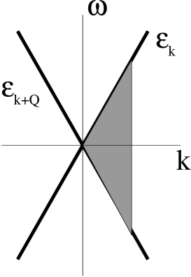
FIG. 4.: Available phase space for particle hole excitations with momentum $Q=2k_{F}$ and energy less or equal to $\omega$. One of the two branches of the electronic band has been displaced by $Q$.

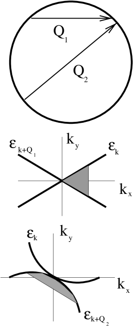
FIG. 5.: Circular Fermi surface (top) and the two possible behaviors of ${\rm Im}\chi({\bf Q},\omega)$ at low energies. Middle: Generic case of non parallel patches of the Fermi surface. Shaded area is the available phase space. Bottom: Wavevector $Q_{2}$ which connects two regions where the Fermi surface is parallel in the two patches.

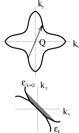
FIG. 6.: Top: Anisotropic Fermi surface with inflection points. Bottom: Available phase space when $Q$ connects two inflection points.

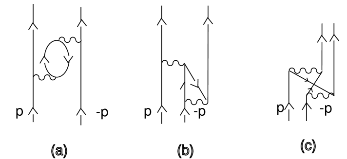
FIG. 7.: Diagrams building up the effective interaction in the BCS channel.

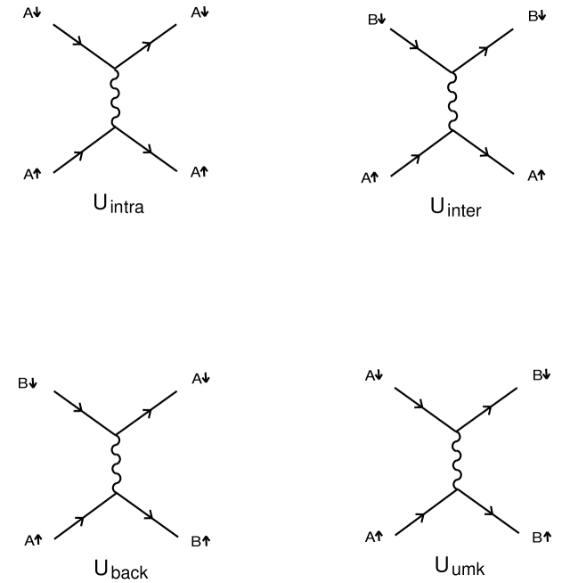
FIG. 8.: Different interaction terms arising from the flavor indices A and B .

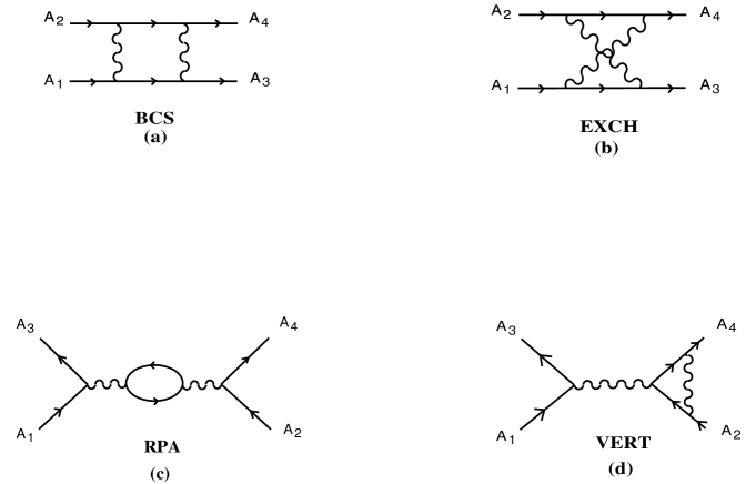
FIG. 9.: Diagrams contributing to the one-loop order correction to the interaction potential.

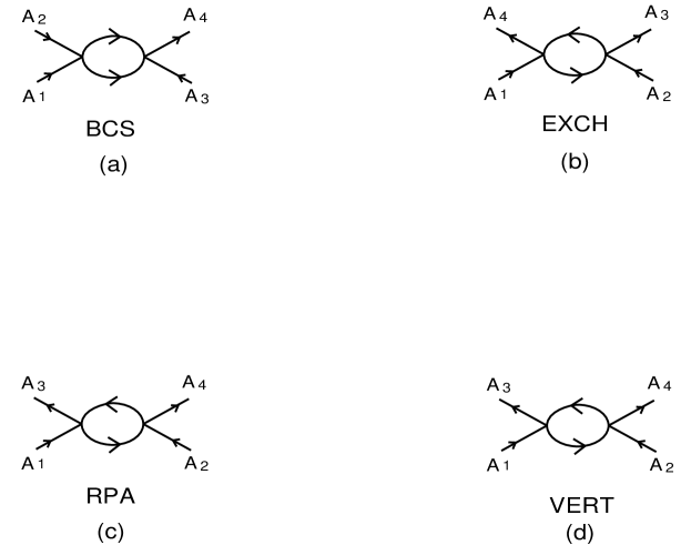
FIG. 10.: Diagrams of Fig. 9 with the interaction shrunk to a point.

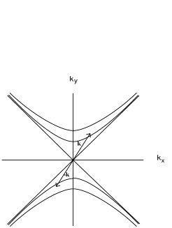
FIG. 11.: Two energy slices used in the computation of the BCS graph.

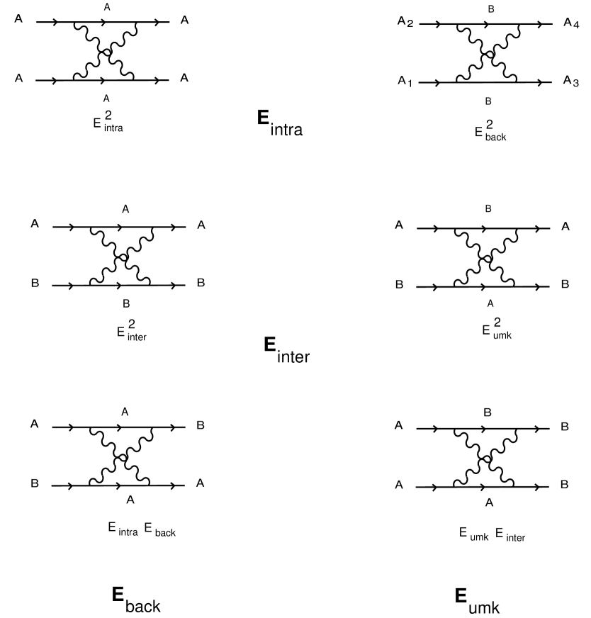
FIG. 12.: Renormalization of the different couplings described in the text.

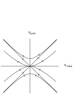
FIG. 13.: The flow of the V couplings described in the text.

REFERENCES

- [1] N. F. Mott, Proc. Phys. Soc. London A62, 416 (1949); Metal-Insulator Transitions, 2nd ed. (Taylor and Francis, London, 1990).
- [2] P. W. Anderson, Science 235, 1196 (1987).
- [3] Z.-X. Shen et al., Science 267, 343 (1995), and references therein.
- [4] B. O. Wells et al., Phys. Rev. Lett. 74, 964 (1995).
- [5] K. Gofron et al., Phys. Rev. Lett. 73, 3302 (1994).
- [6] R. Shankar, Rev. Mod. Phys. 66, 129 (1994).
- [7] W. Kohn and J. M. Luttinger, Phys. Rev. Lett. 15, 524 (1965).
- [8] A more recent account of the subject has been given by M. A. Baranov, A. V. Chubukov and M. Yu. Kagan, Int. J. Mod. Phys. B6, 2471 (1992).
- [9] An elaboration from the point of view of the renormalization group approach can be found in Ref. [6].
- [10] M. A. Baranov and M. Yu. Kagan, Sov. Phys.-JETP 72, 689 (1991).
- [11] A. V. Chubukov, Phys. Rev. B48, 1097 (1993).
- [12] M. A. Baranov and M. Yu. Kagan, Zeit. Phys. B 86, 237 (1992).
- [13] A. V. Chubukov and J. P. Lu, Phys. Rev. B46, 11163 (1992).
- [14] See also R. Hlubina, Phys. Rev. B59, 9600 (1999).
- [15] A. Nazarenko et al., Phys. Rev. B51, 8676 (1995).
- [16] J. González, F. Guinea and M. A. H. Vozmediano, Phys. Rev. Lett. 79, 3514 (1997).
- [17] J. González, F. Guinea and M. A. H. Vozmediano, Europhys. Lett. 34, 711 (1996); report cond-mat/9502095.
- [18] D. M. Newns et al., Phys. Rev. Lett. 69, 1264 (1992).
- [19] D. Z. Liu and K. Levin, Physica 275C, 81 (1997).
- [20] D. Zanchi and H. J. Schulz, Phys. Rev. B54, 9509 (1996).
- [21] R. S. Markiewicz and B. G. Giessen, Physica 160C, 497 (1989).
- [22] P. C. Pattnaik et. al., Phys. Rev. B45, 5714 (1992).
- [23] A complete review of the Van Hove scenario for high- superconductivity is R. S. Markiewicz, J. Phys. Chem. Sol. 58, 1179 (1997).
- [24] J. V. Alvarez, J. González, F. Guinea and M. A. H. Vozmediano, J. Phys. Soc. Jpn. 67, 1868 (1998).
- [25] J. Polchinski, in Proceedings of the 1992 TASI in Elementary Particle Physics, J. Harvey and J. Polchinski eds. (World Scientific, Singapore, 1992).
- [26] This is done, in general, through the characterization of the kind of Fermi liquid proposed by P.-A. Bares and X. G. Wen, Phys. Rev. B48, 8636 (1993).
- [27] We follow at this point the developments in Refs. [6] and [25].
- [28] W. Metzner, C. Castellani and C. Di Castro, Adv. Phys. 47, 3 (1998).
- [29] N. Furukawa, T. M. Rice and M. Salmhofer, Phys. Rev. Lett. 81, 3195 (1998).
- [30] H. J. Schulz, Europhys. Lett. 4, 609 (1987).
- [31] P. Lederer, G. Montambaux and D. Poilblanc, J. Phys. (Paris) 48, 1613 (1987).
- [32] J. E. Dzyaloshinskii, Pis’ma Zh. Eksp. Teor. Fiz. 46, 97 (1987) [JETP Lett. 46, 118 (1987)].
- [33] K. Ueda and T. M. Rice, Phys. Rev. B29, 1514 (1984).
- [34] C. Castellani, C. Di Castro and W. Metzner, Phys. Rev. Lett. 72, 316 (1994).
- [35] J. Labbé and J. Bok, Europhys. Lett. 3, 1225 (1987). J. Friedel, J. Phys. (Paris) 48, 1787 (1987); 49, 1435 (1988).
- [36] R. S. Markiewicz, J. Phys. Condens. Matter 2, 665 (1990).
- [37] C. C. Tsuei et al., Phys. Rev. Lett. 65, 2724 (1990).
- [38] L. B. Ioffe and A. J. Millis, Phys. Rev. B 54, 3645 (1996).
- [39] J. González, F. Guinea and M. A. H. Vozmediano, Nucl. Phys. B 485, 694 (1997).
- [40] J. Sólyom, Adv. Phys. 28, 201 (1979). V. J. Emery, in Highly Conducting One-Dimensional Solids, edited by J. T. Devreese, R. P. Evrard and V. E. Van Doren (Plenum, New York, 1979). H. J. Schulz, “Interacting fermions in one dimension”, report cond-mat/9302006 .
- [41] J. González, M. A. Martín-Delgado, G. Sierra and M. A. H. Vozmediano, Quantum Electron Liquids and High- Superconductivity (Springer-Verlag, Berlin, 1995).
- [42] S. Sorella, R. Hlubina and F. Guinea, Phys. Rev. Lett. 78, 1343 (1997).
- [43] J. V. Alvarez and J. González, Europhys. Lett. 44, 641 (1998).
- [44] J. Betouras and R. Joynt, Europhys. Lett. 31, 119 (1995). Q. P. Li, B. E. C. Koltenbah and R. Joynt, Phys. Rev. B48, 437 (1993). G. Kotliar, Phys. Rev. B37, 3664 (1988). A. E. Ruckenstein, P. J. Hirschfeld and J. Apel, Phys. Rev. B36, 857 (1987).
- [45] J. Ma et al., Science 267, 862 (1995). R. J. Kelley et al., Science 271, 1255 (1996).
- [46] Y. Zhu et al., Phys. Rev. B57, 8601 (1998); Y. N. Tsay et al., in Superconducting Superlattices II: Native and Artificial, I. Bozovic and D. Pavuna, editors, Proceedings of SPIE 3480, 21 (1998).
- [47] Y. D. Chuang et al., report cond-mat/9904050.
- [48] J. González, F. Guinea and M. A. H. Vozmediano, report cond-mat/9905166.
- [49] C. J. Halboth and W. Metzner, report cond-mat/9908471.
- [50] C. Honerkamp et al., report cond-mat/9912358.