Exact Potts Model Partition Functions on Ladder Graphs

Abstract

We present exact calculations of the partition function $Z$ of the $q$-state Potts model and its generalization to real $q$, the random cluster model, for arbitrary temperature on $n$-vertex ladder graphs with free, cyclic, and Möbius longitudinal boundary conditions. These partition functions are equivalent to Tutte/Whitney polynomials for these graphs. The free energy is calculated exactly for the infinite-length limit of these ladder graphs and the thermodynamics is discussed. By comparison with strip graphs of other widths, we analyze how the singularities at the zero-temperature critical point of the ferromagnet on infinite-length, finite-width strips depend on the width. We point out and study the following noncommutativity at certain special values $q_{s}$: $\lim_{n\to\infty}\lim_{q\to q_{s}}Z^{1/n}\neq\lim_{q\to q_{s}}\lim_{n\to\infty}Z^{1/n}$. It is shown that the Potts/random cluster antiferromagnet on both the infinite-length line and ladder graphs with cyclic or Möbius boundary conditions exhibits a phase transition at finite temperature if $0<q<2$, but with unphysical properties, including negative specific heat and non-existence, in the low-temperature phase, of an $n\to\infty$ limit for thermodynamic functions that is independent of boundary conditions. Considering the full generalization to arbitrary complex $q$ and temperature, we determine the singular locus ${\cal B}$ in the corresponding ${\mathbb{C}}^{2}$ space, arising as the accumulation set of partition function zeros as $n\to\infty$. In particular, we study the connection with the $T=0$ limit of the Potts antiferromagnet where ${\cal B}$ reduces to the accumulation set of chromatic zeros. Certain properties of the complex-temperature phase diagrams are shown to exhibit close connections with those of the model on the square lattice, showing that exact solutions on infinite-length strips provide a way of gaining insight into these complex-temperature phase diagrams.

I Introduction

The $q$-state Potts model has served as a valuable model for the study of phase transitions and critical phenomena [1, 2]. On a lattice, or, more generally, on a graph $G$, at temperature $T$, this model is defined by the partition function

$$Z(G,q,v)=\sum_{\{\sigma_{n}\}}e^{-\beta{\cal H}}$$ (1)

with the (zero-field) Hamiltonian

$${\cal H}=-J\sum_{\langle ij\rangle}\delta_{\sigma_{i}\sigma_{j}}$$ (2)

where $\sigma_{i}=1,...,q$ are the spin variables on each vertex $i\in G$; $\beta=(k_{B}T)^{-1}$; and $\langle ij\rangle$ denotes pairs of adjacent vertices. The graph $G=G(V,E)$ is defined by its vertex set $V$ and its edge set $E$; we denote the number of vertices of $G$ as $n=n(G)=|V|$ and the number of edges of $G$ as $e(G)=|E|$. We use the notation

$$K=\beta J$$ (3)

$$a=u^{-1}=e^{K}$$ (4)

and

$$v=a-1$$ (5)

so that the physical ranges are (i) $a\geq 1$, i.e., $v\geq 0$ corresponding to $\infty\geq T\geq 0$ for the Potts ferromagnet, and (ii) $0\leq a\leq 1$, i.e., $-1\leq v\leq 0$, corresponding to $0\leq T\leq\infty$ for the Potts antiferromagnet. An equivalent expression for $Z$ is

$$Z(G,q,v)=\sum_{\{\sigma_{i}\}}\prod_{\langle ij\rangle}(1+v\delta_{\sigma_{i},\sigma_{j}})\ .$$ (6)

One defines the (reduced) free energy per site $f=-\beta F$, where $F$ is the actual free energy, via

$$f(\{G\},q,v)=\lim_{n\to\infty}\ln[Z(G,q,v)^{1/n}]\ .$$ (7)

Let $G^{\prime}=(V,E^{\prime})$ be a spanning subgraph of $G$, i.e. a subgraph having the same vertex set $V$ and an edge set $E^{\prime}\subseteq E$. Then $Z(G,q,v)$ can be written as the sum [3]-[6]

$$Z(G,q,v)=\sum_{G^{\prime}\subseteq G}q^{k(G^{\prime})}v^{e(G^{\prime})}$$ (8)

where $k(G^{\prime})$ denotes the number of connected components of $G^{\prime}$. The formula (8) enables one to generalize $q$ from ${\mathbb{Z}}_{+}$ to ${\mathbb{R}}_{+}$ (keeping $v$ in its physical range). This generalization is the random cluster model [6]. The formula (8) shows that $Z(G,q,v)$ is a polynomial in $q$ and $v$ (equivalently, $a$) with maximum degrees $\max\{deg_{q}(Z(G,q,v))\}=n(G)$ and $\max\{deg_{v}(Z(G,q,v))\}=e(G)$. The minumum degrees are $\min\{deg_{q}(Z(G,q,v))\}=k(G)$, which is equal to 1 for the graphs of interest here (since they are connected), and $\min\{deg_{v}(Z(G,q,v))\}=0$, so

$$Z(G,q,v)=\sum_{r=k(G)}^{n(G)}\sum_{s=0}^{e(G)}z_{rs}q^{r}v^{s}$$ (9)

with $z_{rs}\geq 0$.

The Potts model partition function on a graph $G$ is essentially equivalent to the Tutte polynomial [7]-[11] and Whitney rank polynomial [4], [2], [12]-[14] for this graph, as discussed in the appendix. As a consequence, there are many interesting connections between properties of this partition function and various graph-theoretic quantities.

The Potts model has never been solved exactly for arbitrary temperature on lattices of dimensionality $d\geq 2$ except for special $d=2$, $q=2$ case in which it is equivalent to the solvable 2D Ising model [15] (with the redefinition $J_{Potts}=2J_{Ising}$). Knowledge about the Potts model includes exact calculations of the critical exponents and critical value of the free energy for the 2D ferromagnet for the range $q\leq 4$ where it has a second-order transition; conformal algebra properties for the same range of $q$; the latent heat at the transition point for $q\geq 5$; and certain formulas for the critical point [2, 16]. There is thus motivation for studies that can give further insight into the Potts model. Among these are exact results for the partition function and free energy that one can obtain for infinite-length, finite-width strips with various boundary conditions. We shall present such results in this paper.

One of the interesting features of the Potts model is that the antiferromagnet (AF) exhibits nonzero ground state entropy (without frustration) for sufficiently large $q$ on a given lattice or graph $G$, and serves as a valuable model for the study of this phenomenon. The phenomenon of nonzero ground state entropy, $S_{0}>0$, is an exception to the third law of thermodynamics [17, 18]. This is equivalent to a ground state degeneracy per site (vertex), $W>1$, since $S_{0}=k_{B}\ln W$. The zero-temperature partition function of the above-mentioned $q$-state Potts antiferromagnet (PAF) on $G$ satisfies

$$Z(G,q,T=0)_{PAF}\equiv Z(G,q,v=-1)=P(G,q)$$ (10)

where $P(G,q)$ is the chromatic polynomial (in $q$) expressing the number of ways of coloring the vertices of the graph $G$ with $q$ colors such that no two adjacent vertices have the same color [3, 19, 20]. The minimum (integral) number of colors necessary for this coloring is the chromatic number of $G$, denoted $\chi(G)$. Thus

$$W(\{G\},q)=\lim_{n\to\infty}P(G,q)^{1/n}$$ (11)

where we use the symbol $\{G\}$ to denote $\lim_{n\to\infty}G$ for a given family of graphs.

Since $Z(G,q,v)$ is a polynomial in $q$ and $v$, or equivalently, $a$, one can generalize $q$ from ${\mathbb{Z}}_{+}$ not just to ${\mathbb{R}}_{+}$ but to ${\mathbb{C}}$ and $a$ from its physical ferromagnetic and antiferromagnetic ranges $1\leq a\leq\infty$ and $0\leq a\leq 1$ to $a\in{\mathbb{C}}$. A subset of the zeros of $Z$ in the two-complex dimensional space ${\mathbb{C}}^{2}$ defined by the pair of variables $(q,a)$ can form an accumulation set in the $n\to\infty$ limit, denoted ${\cal B}$, which is the continuous locus of points where the free energy is nonanalytic. As will be discussed below, this locus is determined as the solution to a certain $\{G\}$-dependent equation. For a given value of $a$, one can consider this locus in the $q$ plane, and we denote it as ${\cal B}_{q}(\{G\},a)$. In the special case $a=0$ ($v=-1$) where the partition function is equal to the chromatic polynomial, the zeros in $q$ are the chromatic zeros, and ${\cal B}_{q}(\{G\},a=0)$ is their continuous accumulation set in the $n\to\infty$ limit [22]- [47]; we have determined these accumulation sets exactly for various families of graphs in a series of papers. Other properties of chromatic zeros such as zero-free regions for general graphs, are of mathematical interest (see, e.g., [5, 28, 48]), although we shall not focus on them here. For a given value of $q$, we shall study the continuous accumulation set of the zeros of $Z(G,q,v)$ in the $a$ plane; this will be denoted ${\cal B}_{a}(\{G\},q)$. It will often be convenient to consider the equivalent locus in the $u=1/a$ plane, namely ${\cal B}_{a}(\{G\},q)$. We shall sometimes write ${\cal B}_{q}(\{G\},a)$ simply as ${\cal B}_{q}$ when $\{G\}$ and $q$ are clear from the context, and similarly with ${\cal B}_{a}$ and ${\cal B}_{a}$. A subtlety in the definition of this locus will be discussed in the next section.

One gains a unified understanding of the separate loci ${\cal B}_{q}(\{G\})$ for fixed $a$ and ${\cal B}_{a}(\{G\})$ for fixed $q$ by relating these as different slices of the locus ${\cal B}$ in the ${\mathbb{C}}^{2}$ space defined by $(q,a)$. This is similar to the insight that one gained in studies of accumulation sets of zeros of the partition functions of the Ising model in the ${\mathbb{C}}^{2}$ space defined by $(a,\mu)$, where $\mu=e^{-2\beta H}$ with $H$ being the external field [49, 50], which generalized the Yang-Lee zeros (zeros in $\mu$ for fixed physical $a$) [51] and Fisher zeros (zeros in $a$ for fixed $H$, often $H=0$) [52].

In our earlier works on ${\cal B}_{q}(\{G\})$ for $a=0$, we had denoted the maximal region in the complex $q$ plane to which one can analytically continue the function $W(\{G\},q)$ from physical values where there is nonzero ground state entropy as $R_{1}$. The maximal value of $q$ where ${\cal B}$ intersects the (positive) real axis was labelled $q_{c}(\{G\})$. Thus, region $R_{1}$ includes the positive real axis for $q>q_{c}(\{G\})$. Correspondingly, in our works on complex-temperature properties of spin models, we had labelled the complex-temperature extension (CTE) of the physical paramagnetic phase as (CTE)PM, which will simply be denoted PM here, the extension being understood, and similarly with ferromagnetic (FM) and antiferromagnetic (AFM); other complex-temperature phases, having no overlap with any physical phase, were denoted $O_{j}$ (for “other”), with $j$ indexing the particular phase [54]. Here we shall continue to use this notation for the respective slices of ${\cal B}$ in the $q$ and $a$ or $u$ planes.

In this paper we shall present exact calculations of the Potts/random cluster partition function for strips of the square lattice with arbitrary length $L_{x}$ and width $L_{y}=2$, i.e ladder graphs, having free, periodic (= cyclic), and Möbius longitudinal ($x$-direction) boundary conditions. These families of graphs are denoted, respectively, as $S_{m}$ (for open strip), $L_{m}$ (for ladder), and $ML_{m}$ (for Möbius ladder), where $L_{x}=m+1$ for $S_{m}$ (following our labelling convention in [32]) and $L_{x}=m$ for $L_{m}$ and $ML_{m}$. One has $n(S_{m})=2(m+2)$ and $n(L_{m})=n(ML_{m})=2m$. It will also be instructive to use the well-known solutions for the partition function on the tree and circuit graphs to illustrate some points. We shall discuss several items and investigate several questions about the Potts/random cluster model:

1. We analyze the thermodynamic behavior of the Potts model (for $q\geq 2$) on the infinite-length, $L_{y}=2$ strip and compare it with the known behavior on the line. In particular, we study the zero-temperature critical point of the Potts ferromagnet and discuss how the critical singularities (which are essential singularities in temperature) depend on $q$ and the width of the strip. For reference, one may recall that as one part of his original paper, Onsager used his closed-form solution to the partition function of the Ising model to study it for $L_{y}\times\infty$ strips of the square lattice [15]. The difference, of course, is that for the Potts model with $q\neq 2$, one does not have a general closed-form solution for $Z$ on a $L_{y}\times L_{x}$ grid with arbitrary $L_{y}$ and $L_{x}$; indeed if one did, one would have solved the model on the square lattice.

2. We shall show that the Potts/random cluster model with $0<q<2$ on the $n\to\infty$ limit of the circuit, ladder, and Möbius ladder graphs exhibits a finite-temperature phase transition but with unphysical properties in the low-temperature phase, including negative specific heat, negative partition function, and non-existence of an $n\to\infty$ limit that is independent of boundary conditions.

3. We shall point out and illustrate a certain noncommutativity in the definition of the free energy for the Potts/random cluster model.

4. For a given family of graphs $G$ and its $n\to\infty$ limit, $\{G\}$, we shall explore the nature of the nonanalyticities of the free energy in $q$ and the temperature variable $u$. Some questions related to this are: what is the locus ${\cal B}_{q}$ for various values of $u$ and the locus ${\cal B}_{u}$ for various values of $q$ (and the loci $({\cal B}_{u})_{qn}$ and $({\cal B}_{u})_{nq)}$, for the special values $q=q_{s}$ where these differ)? The strip graphs that we consider here are useful for this study since they are wide enough to exhibit a number of important features but narrow enough so that the terms, denoted $\lambda_{j}$, whose powers contribute to the partition function for a given family of graphs (see eq. (29)) can be calculated as explicit algebraic functions. As our previous studies of asymptotic limits of chromatic polynomials on various infinite-length, finite-width strips have shown [32, 37, 41, 43], as the width of the strip increases, one encounters algebraic equations defining the $\lambda_{j}$’s that increase in degree so that these $\lambda_{j}$ can involve cube roots, fourth roots, and, for equations higher than fourth degree, one cannot obtain exact analytic expressions for them, making it more cumbersome to calculate the locus ${\cal B}$, which is the solution to the degeneracy in magnitude of different dominant $\lambda_{j}$’s.

5. Starting from our previous determination of ${\cal B}_{q}(\{G\})$ for the zero-temperature limit of the Potts antiferromagnet, we explore how this locus changes as on increases $T$ in the range $0<T\leq\infty$. In cases where this locus separates the $q$ plane into different regions for $T=0$, does it continue to do so? How does the point $q_{c}(\{G\})$ vary with temperature? Since we are now dealing with a singular locus in ${\mathbb{C}}^{2}$, we can investigate how the various features of the slice of ${\cal B}(\{G\})$ in the $q$ plane relate to features of the slice ${\cal B}(\{G\})$ in the plane of the temperature variable, $u$ (or the equivalent variable $a$).

6. We shall show that certain features of the complex-temperature phase diagrams of the infinite-length, finite-width strip graphs considered here can give insight into analogous features of the Potts model on the square lattice.

7. Just as was true for our earlier studies of chromatic polynomials and their asymptotic limits, it is of interest to explore the effects of different boundary conditions on the singular locus ${\cal B}(\{G\})$, and we do this.

8. For mathematically inclined readers, we shall give the Tutte polynomials that are equivalent to the Potts model partition functions that we have calculated for the cyclic and Möbius strip graphs and extract special values that are of specific graph-theoretic interest.

Conference reports on some of the material in this paper were given in [43, 44]. In collaboration with H. Kluepfel, we have also carried out calculations of Potts/random cluster partition functions for general $T$ and $q$ on finite patches of several 2D lattices [45] (see also [53]); our work here complements these calculations on finite patches in that we obtain exact results for strip graphs of arbitrarily great length, and the nonanalyticities in the limit $n\to\infty$.

II Some General Considerations

A Basic Properties of $Z$

For our later analysis, it will be useful to record some basic properties of the Potts model partition function. Assuming $q>0$, one observes that for the Potts ferromagnet, since $v>0$, each term in the sum (8) is positive, and consequently, $Z(G,q,v)$ does not have any zeros on the positive real $q$ axis for the physical temperature range. On higher-dimensional lattices where the ferromagnet has a finite-temperature phase transition, zeros will coalesce and pinch the real positive $q$ axis to form a region boundary, but this does not happen in the 1D case and the infinite-length, finite-width strips, which are quasi-1D systems.

One may ask what factors $Z$ has in general. From eq. (8) it follows that for an arbitrary graph $G$,

$$Z(G,q=0,v)=0$$ (12)

and since $Z(G,q,v)$ is a polynomial, this implies that $Z(G,q,v)$ always has an overall factor of $q$. For the families of graphs studied here, this is, in general, the only overall factor that $Z(G,q,v)$ has. For the special case $v=-1$, the resultant chromatic polynomial $Z(G,q,v=-1)=P(G,q)$ has the additional factors $\prod_{s=1}^{\chi(G)-1}(q-s)$. Another general result is that

$$Z(G,q=1,v)=\sum_{G^{\prime}\subseteq G}v^{e(G^{\prime})}=a^{e(G)}\ .$$ (13)

For temperature $T=\infty$, i.e., $v=0$, we have

$$Z(G,q,v=0)=q^{n(G)}\ .$$ (14)

For the Ising case $q=2$, if $G$ is bipartite,

$$Z(G_{bip.},q=2,a)=a^{2e(G_{b})}Z(G_{bip.},q=2,1/a)$$ (15)

where we have written $Z$ here as a function of $a$. This is the well-known equivalence of the Ising ferromagnet (F) and antiferromagnet (AF) on a bipartite lattice, when one makes the replacement $J\to-J$, and hence $K\to-K$, $a\to 1/a$. As a consequence, the zeros of $Z$ in $a$ for $q=2$ are invariant under the inversion mapping $a\to 1/a$. Among the families of graphs considered here, the following are bipartite (equivalently, have chromatic number $\chi=2$): tree graph $T_{m}$ for any $m$; circuit graph $C_{m}$ and cyclic ladder graph $L_{m}$ with $L_{y}=2$ for even $m$; and Möbius ladder graph $ML_{m}$ for odd $m$. In contrast, the cyclic ladder graph $L_{m}$ for odd $m$ and the Möbius ladder graph $ML_{m}$ for even $m$ have $\chi=3$.

For a strip of the square lattice with width $L_{y}$ and cyclic or Möbius longitudinal boundary conditions, the average coordination number (degree in the graph-theoretic terminology) $\Delta_{ave.}=2\lim_{n(G)\to\infty}e(G)/n(G)$ is

$$\Delta_{ave.}=4-\frac{2}{L_{y}}\ .$$ (16)

For the corresponding strip of width $L_{y}$ and free boundary conditions, this formula for $\Delta$ also holds in the $L_{x}\to\infty$ limit. Another consequence of the symmetry (15) is that for the Ising case the internal energy $U$ and specific heat $C$ satisfy the relations

$$U(G_{bip},q=2,J)_{F}=U(G_{bip.},q,J\to-J)_{AF}-\frac{\Delta_{ave.}J}{2}$$ (17)

and

$$C(G_{bip},q=2,J)_{F}=C(G_{bip.},q,J\to-J)_{AF}$$ (18)

(where we have taken the $n\to\infty$ limit, in which these results are independent of the boundary conditions for physical values of temperature).

Another basic property, evident from eq. (8), is that (i) the zeros of $Z(G,q,v)$ in $q$ for real $v$ and hence also the continuous accumulation set ${\cal B}_{q}$ are invariant under the complex conjugation $q\to q^{*}$; (ii) the zeros of $Z(G,q,v)$ in $v$ or equivalently $a$ for real $q$ and hence also the continuous accumulation set ${\cal B}_{a}$ are invariant under the complex conjugation $a\to a^{*}$.

B Noncommutativity in the Random Cluster Model

Just as we showed the importance of noncommutative limits in our earlier work on chromatic polynomials (eq. (1.9) in Ref. [21]), so also we encounter an analogous noncommutativity here for the general partition function (8) of the random cluster model: at certain special points $q_{s}$ (typically $q_{s}=0,1...,\chi(G)$) one has

$$\lim_{n\to\infty}\lim_{q\to q_{s}}Z(G,q,v)^{1/n}\neq\lim_{q\to q_{s}}\lim_{n\to\infty}Z(G,q,v)^{1/n}\ .$$ (19)

Clearly, no such issue of noncommutativity arises if one restricts to positive integer $q$ values and uses the Potts model definition (1), (2). However, for the general random cluster model, whenever $Z(G,q,v)$ has a factor $(q-q_{s})^{\mu_{s}}$ with finite multiplicity $\mu_{s}$ (where typically $\mu_{s}=1$ here), one encounters this noncommutativity. It can also occur when such a factor appears as a coefficient of one of the terms $(\lambda_{G,j})^{m}$ contributing to $Z(G,q,v)$ (see eq. (29) below). The reason for this noncommutativity is analogous to that which we discussed earlier in the special case ($a=0$) of the chromatic polynomial [21]; it is a consequence of the basic result

$$\lim_{n\to\infty}(q-q_{s})^{\mu_{s}/n}=\cases{1&if $q\neq q_{s}$\cr 0&if $q=q_{s}$\cr}\ .$$ (20)

We shall illustrate this with our exact results to be discussed below. Because of this noncommutativity, the formal definition (7) is, in general, insufficient to define the free energy $f$ at these special points $q_{s}$; it is necessary to specify the order of the limits that one uses in eq. (19). We denote the two definitions using different orders of limits as $f_{qn}$ and $f_{nq}$:

$$f_{nq}(\{G\},q,v)=\lim_{n\to\infty}\lim_{q\to q_{s}}n^{-1}\ln Z(G,q,v)$$ (21)

$$f_{qn}(\{G\},q,v)=\lim_{q\to q_{s}}\lim_{n\to\infty}n^{-1}\ln Z(G,q,v)\ .$$ (22)

For the zero-temperature Potts/random cluster antiferromagnet case $a=0$ ($v=-1$), the same ordering ambiguity affects the formal equation (11). In Ref. [21] and our subsequent works on chromatic polynomials and the above-mentioned zero-temperature antiferromagnetic limit, it was convenient to use the ordering $W(\{G\},q_{s})=\lim_{q\to q_{s}}\lim_{n\to\infty}P(G,q)^{1/n}$ since this avoids certain discontinuities in $W$ that would be present with the opposite order of limits. In the present work on the full temperature-dependent random cluster model partition function, we shall consider both orders of limits and comment on the differences where appropriate. Of course in discussions of the usual $q$-state Potts model (with positive integer $q$), one automatically uses the definition in eq. (1) with (2) and no issue of orders of limits arises, as it does in the random cluster model with real $q$.

As a consequence of the noncommutativity (19), it follows that for the special set of points $q=q_{s}$ one must distinguish between (i) $({\cal B}_{a}(\{G\},q_{s}))_{nq}$, the continuous accumulation set of the zeros of $Z(G,q,v)$ obtained by first setting $q=q_{s}$ and then taking $n\to\infty$, and (ii) $({\cal B}_{a}(\{G\},q_{s}))_{qn}$, the continuous accumulation set of the zeros of $Z(G,q,v)$ obtained by first taking $n\to\infty$, and then taking $q\to q_{s}$. For these special points,

$$({\cal B}_{a}(\{G\},q_{s}))_{nq}\neq({\cal B}_{a}(\{G\},q_{s}))_{qn}\ .$$ (23)

From eq. (12), it follows that for any $G$,

$$\exp(f_{nq})=0\quad{\rm for}\quad q=0$$ (24)

and thus

$$({\cal B}_{a})_{nq}=\emptyset\quad{\rm for}\quad q=0\ .$$ (25)

However, for many families of graphs, including the circuit graph $C_{n}$, and cyclic and Möbius strips $L_{m}$ and $ML_{m}$, if we take $n\to\infty$ first and then $q\to 0$, we find that $({\cal B}_{a})_{qn}$ is nontrivial. For these families of graphs, with this order of limits, although the free energy is nonanalytic at $q=0$, it is continuous, and we find that, in general, $\exp(f_{qn})\neq 0$ at $q=0$. Similarly, from (13) we have, for any $G$,

$$({\cal B}_{a})_{nq}=\emptyset\quad{\rm for}\quad q=1$$ (26)

since all of the zeros of $Z$ occur at the single discrete point $a=0$ (and in the case of a graph $G$ with no edges, $Z=1$ with no zeros). However, as the simple case of the circuit graph below will show, $({\cal B}_{a})_{qn}$ is, in general, nontrivial.

We shall also find that $({\cal B}_{a})_{nq}\neq({\cal B}_{a})_{qn}$ for $q=2$ for the infinite-length, $L_{y}=2$ width strip graphs $\{L\}$ and $\{ML\}$. As stated, this noncommutativity can, in general, occur at integer values of $q$ up to and including $q=\chi(G)$. However, although $\chi=3$ for $C_{m}$ and $L_{m}$ with odd $m$ and for $ML_{m}$ with even $m$, there is no noncommutativity at $q=3$ in these cases. This can be seen as a consequence of the fact that one can take the limit $m\to\infty$ on even values of $m$.

In the $q=2$ Ising case, as a consequence of the relation (15), the locus $({\cal B}_{a})_{nq}$ is invariant under the inversion map $a\to 1/a$ for the $n\to\infty$ limit of a sequence of bipartite graphs of type $G$:

$$({\cal B}_{a})_{nq}(\{G_{bip.}\})\quad{\rm is\ invariant\ under}\quad a\to\frac{1}{a}\quad{\rm if}\quad q=2$$ (27)

where $\{G_{bip.}\}$ means that for the family of graphs of type $G$, one can take the limit $n\to\infty$ with a sequence of bipartite members of the family $G$. (For example, for the circuit graphs $C_{n}$, one can do this by taking $n\to\infty$ on even values, and so forth for other families.) As our explicit results for the strips $\{L\}$ and $\{ML\}$ below will show, the locus obtained with the opposite order of limits, $({\cal B}_{a})_{nq}(\{G_{bip.}\})$, does not, in general, have this inversion symmetry, even if $q=2$.

Concerning the cases where the continuous locus ${\cal B}$ may be the nullset $\emptyset$, some examples from chromatic polynomials may be useful. For the complete graph on $n$ vertices $K_{n}$ (defined as the graph in which each point is connected to every other point with edges), if $a=0$, then $Z(K_{n},q,v=-1)=P(K_{n},q)=\prod_{s=0}^{n-1}(q-s)$, so that as $n\to\infty$, there is no continous accumulation set of the chromatic zeros, so ${\cal B}_{q}=\emptyset$ . Another example is provided by the strip $S_{m}$ (see eq. (91) below).

C Definition of Free Energy for Complex $q$ and $K$

Another matter concerns the definition of $f$ away from physical values of $q$ and $K$, where $Z(G,q,a)$ can be negative or complex. In these ranges of $q$ and $K$, there is no canonical choice of which $1/n$’th root, i.e., which value of $r$, to pick in eq. (21) or (22):

$$Z(G,q,a)^{1/n}=\{|Z(G,q,a)|^{1/n}e^{(\phi+2\pi ir)/n}\}\ ,\quad r=0,\ 1,...,n-1\ .$$ (28)

where $\phi=\arg(Z)$. Thus, we start by considering the free energy $f$ defined for sufficiently large (physical) $T$ and integer $q\geq 2$ and define the maximal region in the $q$ plane for fixed $a$ or in the $a$ plane for fixed $q$ that can be reached by analytic continuation of this function. As noted, this is labelled the region $R_{1}$ in the $q$ plane and the PM phase (and its complex-temperature extension) in the $u$ plane. In these regions, the canonical phase choice in (28) is clearly that given by $r=0$. This would also be true in physical low-temperature broken-symmetry phases such as ferromagnetic (FM) or antiferromagnetic (AFM) phases and their complex-temperature extensions, as discussed in [54]; however, such phases do not occur in the 1D and quasi-1D strip graphs considered here. However, in general, in complex-temperature O phases in the $u$ plane and $R_{j}$ regions with $j\neq 1$ in the $q$ plane, only the quantity $|e^{f}|=\lim_{n\to\infty}|Z(G,q,a)|^{1/n}$ can be determined unambiguously.

D General Form of $Z$ for Recursively Defined Graphs

We find that a general form for the Potts model partition function for the strip graphs considered here, or more generally, for recursively defined families of graphs comprised of $m$ repeated subunits (e.g. the columns of squares of height $L_{y}$ vertices that are repeated $L_{x}$ times to form an $L_{x}\times L_{y}$ strip of a regular lattice with some specified boundary conditions), is

$$Z(G,q,v)=\sum_{j=1}^{N_{\lambda}}c_{G,j}(\lambda_{G,j}(q,v))^{m}$$ (29)

where $N_{\lambda}$ depends on $G$. The formula (29) can be understood from the fact that for the cyclic case, for $q\in{\mathbb{Z}}_{+}$, $Z(G,q,v)$ can be expressed as the trace of a transfer matrix ${\cal T}$:

$$Z(G,q,v)=Tr({\cal T}^{m})\ .$$ (30)

Having obtained $Z(G,q,v)$ in this manner, one can then generalize $q$ from ${\mathbb{Z}}_{+}$ to ${\mathbb{R}}_{+}$. For a strip of a regular lattice, this transfer matrix has dimensions ${\cal N}\times{\cal N}$, where ${\cal N}$ denotes the number of possible spin configurations along a transverse slice of the strip; for example, for the square strips of interest here (or for triangular strips, written in the form of a square strip with additional diagonal edges), ${\cal N}=q^{L_{y}}$. Clearly, ${\cal T}$ is a symmetric matrix each of whose elements is either 1 or a (positive) power of $a=v+1$. For physical temperature, for which $a\geq 0$, ${\cal T}$ is real and hence can be diagonalized by an orthogonal transformation $O$, yielding ${\cal N}$ eigenvalues (some of which may coincide). Generically, the multiplicity of a given eigenvalue $\lambda_{G,j}$, which yields the coefficient $c_{j}$ for these cyclic graphs, depends on $q$ but is independent of $v$. The result (29) applies for both free and periodic transverse boundary conditions, given that one uses periodic (cyclic) longitudinal boundary conditions. Similar arguments based on the transfer matrix yield this result if one uses free transverse and Möbius longitudinal, and periodic transverse and Möbius longitudinal (i.e. Klein bottle) boundary conditions.

For strips with open longitudinal boundary conditions, $Z(G,q,v)$ is not a trace, but instead, is given by

$$Z(G,q,v)=\sum_{{\tilde{\sigma}}_{i},{\tilde{\sigma}}_{f}}\langle\tilde{\sigma}_{i}|{\cal T}^{L_{x}}|\tilde{\sigma}_{f}\rangle$$ (31)

where ${\tilde{\sigma}}_{i}$ and ${\tilde{\sigma}}_{f}$ denote the states of the $L_{y}$ spins on the initial (i) and final (f) transverse edges of the strip. As our explicit solution (given below) for the open ladder graph $S_{m}$ shows, here $c_{j}$ can depend on both $q$ and $v$.

For recursively defined families of graphs $G$, the result (29) is a generalization to the case of the Potts/random cluster model partition function $Z(G,q,v)$ of the Beraha-Kahane-Weiss result [25] that the chromatic polynomial $P(G,q)=Z(G,q,v=-1)$ can be written in the form

$$P(G,q)=\sum_{j=1}^{N_{\lambda,P}}c_{P,G,j}(\lambda_{P,G,j})^{m}\ .$$ (32)

Since $P(G,q)$ is a special case of $Z(G,q)$, it follows that

$$N_{\lambda,P}\leq N_{\lambda}\ .$$ (33)

For example, in two well-known cases, (i) tree graph: $N_{\lambda}=N_{\lambda,P}=1$, (ii) circuit graph: $N_{\lambda}=N_{\lambda,P}=2$. We find (iii) for the open $L_{y}=2$ ladder $S_{m}$, $N_{\lambda}=2$, while $N_{\lambda,P}=1;(iv)forthe$cyclic and Möbius strips, $N_{\lambda}=6$ while [22] $N_{\lambda,P}=4$. For the subset of the $\lambda_{G,j}$’s that remain for $P(G,q)$, the coefficient functions $c_{P,G,j}=c_{G,j}(v=-1)$; as remarked above, for the cyclic case and our Möbius strip, $c_{G,j}$ are independent of $v$.

As $m\to\infty$, for a given point $(q,v)$ in the ${\mathbb{C}}^{2}$ space of variables, one $\lambda_{j}$ will dominate this sum; we denote this as the “leading term” $\lambda_{\ell}$, where $\ell$ stands for leading. As one moves to another point $(q^{\prime},v^{\prime})$, it may happen that there is a change in the dominant $\lambda$, from $\lambda_{\ell}$ to, say, $\lambda_{\ell}^{\prime}$. Consequently, there is a nonanalytic change in the free energy $f$ as it switches from being determined by the first dominant $\lambda_{\ell}$ to being determined by $\lambda_{\ell}^{\prime}$. Thus, the equation for the continuous nonanalytic locus ${\cal B}$ across which $f$ is nonanalytic, is (with the $\{G\}$ dependence indicated explicitly)

$${\cal B}(\{G\}):\quad|\lambda_{G,\ell}|=|\lambda_{G,\ell}^{\prime}|\ .$$ (34)

Although $f$ is nonanalytic across ${\cal B}$, a consequence of eq. (34) is that $|e^{f}|$ is continuous across this locus. This is the generalization of the analogous phenomenon for the asymptotic limit of chromatic polynomials, or equivalently, the $T=0$ limit of the Potts antiferromagnet [25, 26, 28, 21], i.e. the property that $W(\{G\},q)$ is nonanalytic (although its magnitude is continuous) across ${\cal B}_{q}(\{G\})$. As noted above, the locus ${\cal B}$ forms as the continuous accumulation set of the zeros of $Z(G,q,v)$ in the 2-complex dimensional space $(q,v)$ as $n(G)\to\infty$. This again generalizes the earlier analysis for chromatic polynomials, where ${\cal B}_{q}$ formed as the continuous accumulation set of the zeros of the chromatic polynomial in the single complex variable $q$.

It is straightforward to generalize the transfer matrix formalism and hence eqs. (30) and (31) to the case of the Potts model in an external magnetic field $H$, where the Hamiltonian is ${\cal H}=-J\sum_{\langle ij\rangle}\delta_{\sigma_{i}\sigma_{j}}-H\sum_{i}\delta_{\sigma_{i},\sigma_{0}}$ (with $\sigma_{0}$ chosen, say, as 1). Hence, the full generalization for recursively defined families of graphs is, with $\eta=e^{\beta H}$,

$$Z(G,q,v,\eta)=\sum_{j=1}^{N_{\lambda}}c_{G,j}(\lambda_{G,j}(q,v,\eta))^{m}\ .$$ (35)

One could proceed to study the singular locus ${\cal B}$ in the ${\mathbb{C}}^{3}$ space of the variables $(q,v,\eta)$ which forms as the continuous accumulation set of the zeros of $Z$, and the various slices in the $q$, $a$, and $\eta$ planes. Here we restrict ourselves to the zero-field case, $\eta=1$.

Typically, for a given point $a\in{\mathbb{C}}$, there will be an infinite set of points in the $q$ plane lying on ${\cal B}$, and for a given point $q\in{\mathbb{C}}$, there will be an infinite set of points in the $a$ plane lying on ${\cal B}$. Again, usually (we have commented on some exceptions above, where accumulation sets of zeros are discrete), we find that ${\cal B}_{q}$ and ${\cal B}_{a}$ form curves (and possible line segments) in the respective $q$ and $x=a$ or $u$ planes. This follows from the property that ${\cal B}$ is the solution of an algebraic equation expressing the degeneracy of the leading $\lambda$’s contributing to $Z$. (For higher dimensional lattices the equations defining ${\cal B}$ can be transcendental instead of algebraic.) The loci ${\cal B}_{q}$ and ${\cal B}_{x}$, $x=a$ or $u$, may be connected, or may consist of several disconnected components; our results illustrate both types of behavior.

The Potts ferromagnet has a zero-temperature phase transition in the $L_{x}\to\infty$ limit of the strip graphs considered here, and this has the consequence that for cyclic and Möbius boundary conditions, ${\cal B}$ passes through the $T=0$ point $u=0$. It follows that ${\cal B}$ is noncompact in the $a$ plane. Hence, it is usually more convenient to study the slice of ${\cal B}$ in the $u=1/a$ plane rather than the $a$ plane. In the Ising case $q=2$, ${\cal B}_{a}={\cal B}_{u}$ and so both are noncompact. For the ferromagnet, since $a\to\infty$ as $T\to 0$ and $Z$ diverges like $a^{e(G)}$ in this limit, we shall use the reduced partition function $Z_{r}$ defined by

$$Z_{r}(G,q,v)=a^{-e(G)}Z(G,q,v)=u^{e(G)}Z(G,q,v)$$ (36)

which has the finite limit $Z_{r}\to 1$ as $T\to 0$. For a general strip graph $(G_{s})_{m}$ of type $G_{s}$ and length $L_{x}=m$, we can write

$$Z_{r}((G_{s})_{m},q,a) = u^{e((G_{s})_{m})}\sum_{j=1}^{N_{\lambda}}c_{G_{s},j}(\lambda_{G_{s},j})^{m}\equiv\sum_{j=1}^{N_{\lambda}}c_{G_{s},j}(\lambda_{G_{s},j,u})^{m}$$ (37)

with

$$\lambda_{G_{s},j,u}=u^{e((G_{s})_{m})/m}\lambda_{G_{s},j}\ .$$ (38)

For example, for the strips of the square lattice with periodic longitudinal boundary conditions and free transverse boundary conditions, and of width $L_{y}$ vertices, we have $e(sq(L_{y})_{m})=(2L_{y}-1)m$, so the prefactor in (38) is $u^{2L_{y}-1}$.

III 1D Case with Free Boundary Conditions

We first briefly discuss two cases that illustrate some important features in their simplest contexts. We begin with Potts/random cluster model on a line of $n$ vertices, or, more generally, a tree graph, $T_{n}$. One has the well-known result

$$Z(T_{n},q,v)=q(q+v)^{n-1}.$$ (39)

This case illustrates the general feature that the antiferromagnetic random cluster model for real positive non-integral $q$ fails to satisfy the usual statistical mechanical requirement that the partition function is positive, and hence does not, in general admit a Gibbs measure [56]. Specifically, here we have

$$Z(T_{n},q,v)<0\quad{\rm for}\ \ n\ \ {\rm even}\ \ {\rm and}\ \ q+v<0\ .$$ (40)

These negative values of $Z(T_{n},q,v)$ occur at physical finite temperature if $0<q<1$ and $n$ is even, since the condition $q+a-1<0$ is equivalent to $T<T_{un}$, where

$$T_{un}=\frac{J}{k_{B}\ln(1-q)}=\frac{|J|}{k_{B}\ln\Bigl{(}\frac{1}{1-q}\Bigr{)}}\ ,\quad 0<q<1\ ,\quad J<0.$$ (41)

Although in this case one could restore positivity by requiring that $n$ be odd, we shall show that there are further pathologies associated with this temperature.

The continuous locus ${\cal B}=\emptyset$ since the accumulation set of the zeros of $Z$ in $q$ is the discrete point $q=-v$. For $q\neq 0$, the limits in the definitions (22) and (21) commute, and the free energy is (with $v=a-1$)

$$f_{qn}=f_{nq}\equiv f=\ln(q+a-1)\ .$$ (42)

The physical thermodynamic behavior for this case will be compared below with that for the width $L_{y}=2$ strips. For this purpose, we record the internal energy,

$$U=-\frac{Ja}{q+a-1}$$ (43)

and the specific heat,

$$C=\frac{k_{B}K^{2}(q-1)a}{(q+a-1)^{2}}\ .$$ (44)

Note that the specific heat (44) is positive if $q>1$ but is negative and hence unphysical for all temperatures if $q<1$, in both the ferromagnetic and antiferromagnetic cases. Thus the pathological nature of the range $0<q<1$ is manifested in the negative specific heat even for temperatures above the value $T_{un}$ in eq. (40) below which $Z$ can be negative. Also, note that in the antiferromagnetic case there are unphysical divergences of $U$ and $C$ at $T=T_{un}$.

For $q=0$, the noncommutativity (19) occurs, and one has $\exp(f_{nq})=0$ but $\exp(f_{qn})=(a-1)$. This simple case demonstrates that the noncommutativity at a special point $q_{s}$ can occur even when this point is not the the singular locus $({\cal B})_{qn}$ or $({\cal B})_{nq}$. In passing we note that a study of the $q$-state Potts model on the Bethe lattice (tree graph in which the interior vertices all have the same coordination number) has been carried out in [57].

IV 1D Case with Periodic Boundary Conditions

A General

The Potts/random cluster model on the circuit graph $C_{n}$, or equivalently, the 1D line with periodic boundary conditions, is probably the simplest case with a nontrivial locus ${\cal B}$. The Tutte polynomial for this graph is well known [12], and the corresponding Potts model partition function is

$$Z(C_{n},q,a)=(q+v)^{n}+(q-1)v^{n}\ .$$ (45)

As noted above, the Potts ferromagnet has a zero-temperature critical point, and this is also true of the antiferromagnet in the $q=2$ case where these are equivalent. In the antiferromagnetic case, there is nonzero ground state entropy, $S=k_{B}\ln(q-1)$ if $q>2$.

For comparison with the $L_{y}=2$ results to be given below, we recall some of the thermodynamic properties of the 1D Potts model. Here we take $q\geq 2$ where there is no pathological behavior (see below) and restrict to physical values of $J$ and $T$; the resulting thermodynamic functions are then independent of whether one uses periodic or free boundary conditions and were given above for $f$, $U$, and $C$ in eqs. (42)-(44). The internal energy and specific heat have the high-temperature expansions

$$U=-\frac{J}{q}\biggl{[}1+\frac{(q-1)}{q}K+O(K^{2})\biggr{]}$$ (46)

$$C=\frac{k_{B}(q-1)K^{2}}{q^{2}}\biggl{[}1+\frac{(q-2)}{q}K+O(K^{2})\biggr{]}$$ (47)

Recall that the $T\to 0$ limit corresponds to $K\to\infty$, i.e. $u\to 0$, for the ferromagnet ($J>0$) and to $K\to-\infty$, i.e., $a\to 0$, for the antiferromagnet ($J<0$). The low-temperature expansions for these two cases are different:

$$U=-J\biggl{[}1-(q-1)e^{-K}+O(e^{-2K})\biggr{]}\quad{\rm as}\quad K\to\infty$$ (48)

$$U=\frac{(-J)e^{K}}{(q-1)}\biggl{[}1-\frac{1}{q-1}e^{K}+O(e^{2K})\biggr{]}\quad{\rm as}\quad K\to-\infty$$ (49)

$$C=k_{B}(q-1)K^{2}e^{-K}\biggl{[}1-2(q-1)e^{-K}+O(e^{-2K})\biggr{]}\quad{\rm as}\quad K\to\infty$$ (50)

$$C=\frac{k_{B}K^{2}e^{K}}{(q-1)}\biggl{[}1-\frac{2}{q-1}e^{K}+O(e^{2K})\biggr{]}\quad{\rm as}\quad K\to-\infty\ .$$ (51)

Note that in the Ising case $q=2$, these expansions satisfy the symmetry relations (17) and (18).

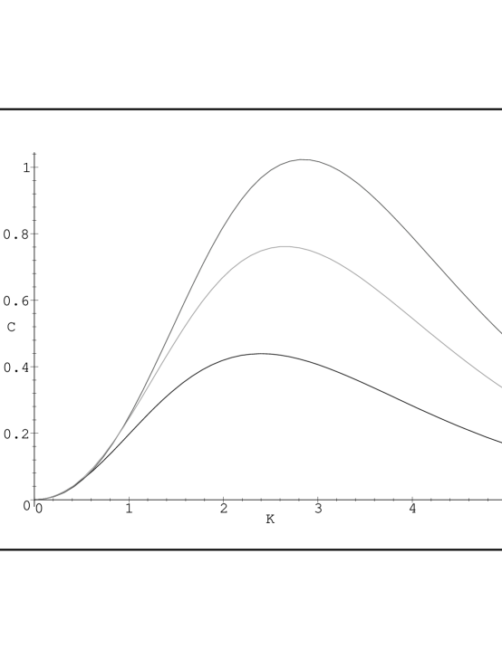
FIG. 1.: Specific heat for the 1D Potts ferromagnet as a function of $K=J/(k_{B}T)$. Going from bottom to top in order of the heights of the maxima, the curves are for $q=2,3,4$.

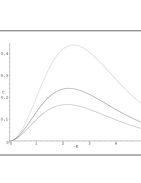
FIG. 2.: Specific heat for the 1D Potts antiferromagnet as a function of $-K=-J/(k_{B}T)$. Going from top to bottom, the curves are for $q=2,3,4$.

In Figs. 1 and 2 we plot $C$ for the ($n\to\infty$ limit of the) ferromagnetic (F) and antiferromagnetic (AF) cases (with $k_{B}=1$). In the antiferromagnetic case, $C$ is a decreasing function of $q$ for all $0<T<\infty$. In the ferromagnetic case, $C$ increases (decreases) with $q$ at low (high) temperatures and the curves for two different values $q=q_{1}$ and $q=q_{2}$ are equal at the temperature $T_{cr}=J/(k_{B}K_{cr})$, where

$$K_{cr}=\frac{1}{2}\ln\Bigl{[}(q_{1}-1)(q_{2}-1)\Bigr{]}\ .$$ (52)

Thus, $K_{cr}\simeq 0.35,\ 0.55,\ 0.90$ for $q=2,3,4$. The specific heat has a maximum at a temperature $K_{cmax}$ given by the solution of the equation $(q-1)(K+2)+(2-K)e^{K}=0$. Some illustrative values for Figs. 1 and 2 are (i) $K_{cmax}\simeq\pm 2.4$ (F,AF) for $q=2$; (ii) $K_{cmax}\simeq 2.7$ (F), $K_{cmax}\simeq-2.2$ (AF) for $q=3$; (iii) $K_{cmax}\simeq 2.85$ (F), $K_{cmax}\simeq-2.15$ (AF) for $q=4$. For $q\geq 3$, the value of $C$ at this maximum increases (decreases) with $q$ for the ferromagnet (antiferromagnet).

B ${\cal B}_{q}(\{C\})$ for fixed $a$

Returning to the study of ${\cal B}_{q}$ in the complex $q$ plane as a function of $a$, we note that the solution of the degeneracy equation $|q+a-1|=|a-1|$ determines the locus ${\cal B}_{q}(\{C\})$ to be the circle centered at $q=1-a$ of radius $|1-a|$:

$$q=(1-a)(1+e^{i\theta})\ ,0\leq\theta<2\pi\ .$$ (53)

For $a<1$ and $a>1$, this circle has support in the right-hand and left-hand half planes $Re(q)\geq 0$ and $Re(q)\leq 0$, respectively; for any $a$, it always passes through the origin. The locus ${\cal B}_{q}$ intersects the real $q$ axis at $q=0$ and at $q=q_{c}(\{C\})$, where

$$q_{c}(\{C\})=2(1-a)\ .$$ (54)

In general, for finite $n$, the zeros of $Z$ do not lie exactly on ${\cal B}$. We have shown, however, that in the $T=0$ limit of the Potts antiferromagnet, i.e., for $a=0$, the zeros of $Z(C_{n},q,a=0)=P(C_{n},q)$ do lie exactly on the locus ${\cal B}$, which, for this case is the circle $|q-1|=1$ [21, 30]. As $T$ increases from 0 to infinity for the Potts antiferromagnet, i.e. as $a$ increases from 0 to 1, the radius and center of the circle both decrease from 1 to 0 so that it contracts to the origin at $a=1$. As $a$ increases above 1 through real values, i.e. as $T$ decreases from $\infty$ to 0 for the ferromagnetic case, the circle is located in the $Re(q)\leq 0$ half-plane, with its center moving leftward and its radius increasing as a function of $a$. In this ferromagnetic case, the crossing point given by $q_{c}(\{C\})$ occurs on the negative real $q$ axis; ${\cal B}_{q}$ does not cross the positive real $q$ axis.

C ${\cal B}_{u}(\{C\})$ for fixed $q$

We first consider values of $q\neq 0,1$, so that no noncommutativity occurs, and $({\cal B}_{u})_{nq}=({\cal B}_{u})_{qn}\equiv{\cal B}_{u}$. As discussed above, it is convenient to use the $u$ plane since ${\cal B}_{u}$ is compact in this plane, except for the case $q=2$, whereas ${\cal B}_{a}$ is noncompact because of the ferromagnetic zero-temperature critical point at $u=1/a=0$. For $q\neq 0,1,2$, ${\cal B}_{u}$ is the circle [58]

$${\cal B}_{u}:\ \ u=\frac{1}{(q-2)}(-1+e^{i\omega})\ ,\quad 0\leq\omega<2\pi\ .$$ (55)

The exterior of this circle is the (complex-temperature extension of the) PM phase, and its interior is an O phase.

For the ferromagnet, the fact that the singular locus ${\cal B}_{u}$ passes through the $T=0$ point $u=0$ for the 1D Potts model with periodic boundary conditions, while for the same model with free boundary conditions, ${\cal B}_{u}$ does not pass through $u=0$, means that the use of periodic boundary conditions yields a singular locus that manifestly incorporates the zero-temperature critical point, while this is not manifest in ${\cal B}_{u}$ when calculated using free boundary conditions. As we shall show, this continues to be true concerning the longitudinal boundary conditions when one considers the Potts ferromagnet on the $L_{y}=2$ strip graphs. This leads us to one of the important conclusions of this work, namely that although calculations of the free energy of the Potts model on infinite-length, finite-width strips with periodic boundary conditions in the longitudinal direction (the direction in which the strip length goes to infinity) are more difficult than with free longitudinal boundary conditions, the extra work is worth it since the resulting locus ${\cal B}$ incorporates this feature of passing through $u=0$, corresponding to the zero-temperature critical point of the ferromagnet, if one uses periodic longitudinal boundary conditions. From our studies in the different, although related, context of chromatic polynomials [36, 37, 41, 42, 43], we reached the analogous conclusion that although the calculation of $P(G,q)$ for strip graphs of a regular lattice is more complicated when one uses periodic longitudinal boundary conditions, the resultant singular locus ${\cal B}_{q}$ has the advantage of incorporating more of the features expected of the infinite-width limit, i.e. the full two-dimensional lattice. One such expectation, based on calculations of chromatic polynomials and the resultant $W$ functions of eq. (11) for infinite-length, finite-width strips as the width increased, was that ${\cal B}_{q}$ passes through $q=0$ and that this nonanalytic locus separates the region including the interval $0<q<q_{c}(\{G\})$ on the real axis from the outlying region for sufficiently large $|q|$ [32, 33]; this is also in agreement with the calculation in [27] for the triangular lattice. However, for finite width strips, ${\cal B}_{q}$ consists of arcs [32] (and possible closed regions, as in Fig. 4 of [33]) which do not pass through $q=0$ and do not have this enclosure property.

The circle (55) crosses the real axis at $u=0$ and at

$$u_{c}(\{C\})=\frac{1}{a_{c}(\{C\})}=-\frac{2}{q-2}$$ (56)

(cf. eq. (54)). The point $u_{c}(\{C\})$ occurs at complex temperature for $q>2$ and physical temperature for $q<2$. We shall comment further below on the case $0<q<2$. In the $a$ plane, ${\cal B}_{a}$ is the vertical line

$${\cal B}_{a}:\ \ Re(a)=a_{c}=1-\frac{q}{2},\quad-\infty\leq Im(a)\leq\infty\ .$$ (57)

The phase with $Re(a)>a_{c}$, to the right of this line, is the (complex-temperature extension of the) PM phase, while the phase to the left of the line is the O phase. As $q\to 2$, the radius of the circle (55) goes to infinity, and at $q=2$, ${\cal B}_{u}$ is identical to ${\cal B}_{a}$ by the symmetry relation (27), forming the full imaginary $u$ axis.

We next consider the special values $q=0$ and 1 for which noncommutativity occurs. For $q=0$, $e^{f_{nq}}=0$ as in (24) while in the PM phase with $Re(a)>1$, $e^{f_{qn}}=a-1$ and in the O phase with $Re(a)<1$, $|e^{f_{qn}}|=|a-1|$; the locus $({\cal B}_{a})_{nq}=\emptyset$, while $({\cal B}_{a})_{qn}$ is given by (57) as the vertical line $Re(a)=1$. For $q=1$, the coefficient multiplying the second term in $Z(C_{n},q,v)$ vanishes, and $Z(G,q=1,v)=a^{n}$, a special case of (13). Here $e^{f_{nq}}=a$ while in the PM phase defined by $Re(a)>a_{c}=1/2$, we have $e^{f_{qn}}=a$ and in the O phase defined by $Re(a)<1/2$, we have $|e^{f_{qn}}|=|a-1|$; $({\cal B}_{a})_{nq}=\emptyset$ since all of the zeros of $Z$ occur at the discrete point $a=0$, while $({\cal B}_{a})_{qn}$ is given by eq. (57) as the vertical line $Re(a)=1/2$.

D Phase Transition for Antiferromagnetic Case with $0<q<2$

For the range $0<q<2$, and the antiferromagnetic case $J<0$, the nonanalyticity in the free energy at $a=a_{c}=(2-q)/2$ in (56) occurs at the physical temperature

$$T_{p}=\frac{|J|}{k_{B}\ln\Big{(}\frac{2}{2-q}\Bigr{)}}\ ,\quad 0<q<2\ .$$ (58)

Therefore, the generalization of the Potts antiferromagnet to real positive $q$ defined by the random cluster representation (8) has a finite-temperature phase transition in the $n\to\infty$ limit of the circuit graph, i.e. in 1D with periodic boundary conditions. (For the special value $q=q_{s}=1$, it is understood that one takes $n\to\infty$ first and then $q\to 1$, i.e., one uses $f_{qn}$; with the other order, $q\to 1$ and then $n\to\infty$, $f_{nq}$ is analytic and there is no phase transition.) The phase transition at $T=T_{p}$ is not a counterexample to the usual theorem that a one-dimensional spin model with short-ranged interactions does not have any phase transition at finite temperature, because the existence of this transition is inextricably connected with the failure of positivity for $Z$ and hence the absence of a Gibbs measure, which are implicit requirements for the applicability of the above-mentioned theorem. As $q$ decreases from 2 to 0, the phase transition temperature $T_{p}$ increases from 0 to infinity.

In the high-temperature paramagnetic phase $T>T_{p}$, the free energy, internal energy, and specific heat are given by the same expressions as for the $n\to\infty$ limit of the Potts/random cluster model on the tree graph, eqs. (42), (43), and (44), respectively. Hence, even in the high-temperature phase, one has an unphysical negative specific heat if $q<1$. In the low-temperature O phase, strictly speaking, only $|Z|$ can be determined: $|\exp(f_{qn})|=|a-1|$, but with an appropriate choice of multiplicative phase, we can choose

$$f=\ln(1-a)\ ,\quad T<T_{p}$$ (59)

and hence

$$U=\frac{Ja}{1-a}\ ,\quad T<T_{p}$$ (60)

$$C=-\frac{k_{B}K^{2}a}{(1-a)^{2}}\ ,\quad T<T_{p}\ .$$ (61)

Thus, for all $q$ in the range $0<q<2$ where there is a finite-temperature phase transition, the low-temperature phase has pathological property that the specific heat is negative. The phase transition itself is first-order, with latent heat

$$\lim_{T\to T_{p}^{+}}U-\lim_{T\to T_{p}^{-}}U=\frac{2|J|(2-q)}{q}\ .$$ (62)

A basic pathology of the low-temperature phase of this antiferromagnet, i.e., the phase where $|v|>|q+v|$, is that $Z$ can be negative. For sufficiently large $n$, this occurs for $1<q<2$ if $n$ is odd and for $0<q<1$ if $n$ is even.

Thus, if one restricts to $q>1$, this 1D antiferromagnetic random cluster model satisfies, at least in the high-temperature phase, the requirement that the specific heat is positive and, for the interval $1<q<2$, has a (first-order) finite-temperature phase transition; however, even if one restricts the approach to the $n\to\infty$ limit to even values of $n$, the low-temperature phase is unphysical because of the negative specific heat. One also observes that the results for the free energy and associated thermodynamic functions are the same for the $n\to\infty$ limit of the tree graph and the circuit graph, i.e. are independent of whether one uses free or periodic boundary conditions, if $T>T_{p}$, but differ for $T<T_{p}$, so that the existence of the low-temperature phase in the case of periodic boundary conditions also means that the $n\to\infty$ limit does not exist owing to different results obtained with different boundary conditions. The non-existence of a well-defined $n\to\infty$ limit for the random cluster model with non-integral $q$ has been noted previously in [56]. For positive integer $q$, the (zero-field) $q$-state Potts model is invariant under the operations of the permutation group $S_{q}$; however, this symmetry group is not defined for non-integral $q$. In any case, the usual Peierls argument shows that even if one could define some notion of a symmetry of $Z$ for non-integral $q$, this symmetry could not be broken spontaneously in the phase transition for this 1D system or, indeed, for the random cluster model on an infinite-length, finite-width strip, to be discussed below.

A further generalization of this 1D random cluster model is to keep $q$ real but let it be negative; in this case the model with the ferromagnetic sign of the coupling, $J>0$, formally has a nonanalyticity in the free energy at a positive finite value of the parameter $T$ given by $k_{B}T=J/\ln[(2-q)/2]$. However, since this model does not, in general, have a positive $Z$, one cannot really refer to this parameter as a physical temperature and we shall not discuss this case further.

E Other slices of ${\cal B}(\{C\})$

So far we have considered the “orthogonal” slices of ${\cal B}$ obtained by holding either $q$ or $q$ constant. A different type of slice is obtained if one has $q$ and $a$ satisfy some functional relation. As an illustration of this, we consider perhaps the simplest case, namely the linear relation $a+q=c$, where $c\in{\mathbb{C}}$ is a constant. If one treats the $a$ and $q$ variables as the “horizontal” and “vertical” axes (actually planes, in terms of real variables), then the condition $a+q=c$ is an affine translation of a diagonal slice of the complex locus ${\cal B}$. The resultant ${\cal B}_{a}$ is the solution of the equation $|c-1|=|a-1|$, which is a circle centered at $a=1$ with radius $|c-1|$. The corresponding ${\cal B}_{q}$ is a circle centered at $q=c-1$ with radius $|c-1|$. These circles in the $a$ and $q$ planes pass through $a=0$ and $q=0$, respectively.

V Square Strip with Free Longitudinal Boundary Conditions

In this section we present the Potts model partition function $Z(S_{m},q,v)$ for the $L_{y}=2$ strip of the square lattice $S_{m}$ with arbitrary length $L_{x}=m+1$ (i.e., containing $m+1$ squares) and free transverse and longitudinal boundary conditions. One convenient way to express the results is in terms of a generating function:

$$\Gamma(S,q,v,z)=\sum_{m=0}^{\infty}Z(S_{m},q,v)z^{m}\ .$$ (63)

We have calculated this generating function using the deletion-contraction theorem for the corresponding Tutte polynomial $T(S_{m},x,y)$ and then expressing the result in terms of the variables $q$ and $v$. We find

$$\Gamma(S,q,v,z)=\frac{{\cal N}(S,q,v,z)}{{\cal D}(S,q,v,z)}$$ (64)

where

$${\cal N}(S,q,v,z)=A_{S,0}+A_{S,1}z$$ (65)

with

$$A_{S,0}=q(v^{4}+4v^{3}+6qv^{2}+4q^{2}v+q^{3})$$ (66)

$$A_{S,1}=-q(v+1)(v+q)^{3}v^{2}$$ (67)

and

$${\cal D}(S,q,v,z)=1-(v^{3}+4v^{2}+3qv+q^{2})z+(v+1)(v+q)^{2}v^{2}z^{2}\ .$$ (68)

(The generating function for the Tutte polynomial $T(S_{m},x,y)$ is given in the appendix.) Writing

$${\cal D}(S,q,v,z)=\prod_{j=1}^{2}(1-\lambda_{S,j}z)$$ (69)

we have

$$\lambda_{S,(1,2)}=\frac{1}{2}(T_{S12}\pm\sqrt{R_{S12}}\ )$$ (70)

where

$$T_{S12}=v^{3}+4v^{2}+3qv+q^{2}$$ (71)

and

$$R_{S12}=v^{6}+4v^{5}-2qv^{4}-2q^{2}v^{3}+12v^{4}+16qv^{3}+13q^{2}v^{2}+6q^{3}v+q^{4}\ .$$ (72)

In [34] we presented a formula to obtain the chromatic polynomial for a recursive family of graphs in the form (32) starting from the generating function. It will be useful to give here the generalization of this formula for the full Potts partition function. For a strip (recursive) graph with the labelling conventions used here, the generating function can be written as

$$\Gamma(G,q,v,z)=\frac{{\cal N}(G,q,v,z)}{{\cal D}(G,q,v,z)}$$ (73)

with

$${\cal N}(G,q,v,z)=\sum_{j=0}^{d_{\cal N}}A_{G,j}z^{j}$$ (74)

and

$${\cal D}(G,q,v,z) = 1+\sum_{j=1}^{d_{\cal D}}b_{G,j}z^{j}$$ (75)

$$= \prod_{j=1}^{d_{\cal D}}(1-\lambda_{G,j}z)$$ (77)

where

$$d_{\cal N}(G)=deg_{z}({\cal N}(G))$$ (78)

$$d_{\cal D}(G)=deg_{z}({\cal D}(G))$$ (79)

Then the formula is

$$Z(G_{m},q,v)=\sum_{j=1}^{d_{\cal D}}\Biggl{[}\sum_{s=0}^{d_{\cal N}}A_{G,j}\lambda_{j}^{d_{\cal D}-s-1}\Biggr{]}\Biggl{[}\prod_{1\leq i\leq d_{\cal D};i\neq j}\frac{1}{(\lambda_{G,j}-\lambda_{G,i})}\Biggr{]}\lambda_{G,j}^{m}$$ (80)

For our present open strip $S_{m}$, we have

$$Z(S_{m},q,v)=\frac{(A_{S,0}\lambda_{S,1}+A_{S,1})}{(\lambda_{S,1}-\lambda_{S,2})}\lambda_{S,1}^{m}+\frac{(A_{S,0}\lambda_{S,2}+A_{S,1})}{(\lambda_{S,2}-\lambda_{S,1})}\lambda_{S,2}^{m}$$ (81)

(which is symmetric under $\lambda_{S,1}\leftrightarrow\lambda_{S,2}$). This shows that the $c_{G,j}$ can depend on both $q$ and $v$ for open strip graphs. Although both the $\lambda_{S,j}$’s and the coefficient functions involve the square root $\sqrt{R_{S12}}$ and are not polynomials in $q$ and $v$, the theorem on symmetric functions of the roots of an algebraic equation [61] guarantees that $Z(S_{m},q,v)$ is a polynomial in $q$ and $v$ (as it must be by (8) since the coefficients of the powers of $z$ in the equation (77) defining these $\lambda_{S,j}$’s are polynomials in these variables $q$ and $v$. This is a generalization of our discussion in [41] from the special case of chromatic polynomials to the general case of the Potts/random cluster partition function.

As will be shown below, the singular locus ${\cal B}_{u}$ consists of arcs that do not separate the $u$ plane into different regions, so that the PM phase and its complex-temperature extension occupy all of this plane, except for these arcs. For physical temperature and positive integer $q$, the (reduced) free energy of the Potts model in the limit $n\to\infty$ is given by

$$f=\frac{1}{2}\ln\lambda_{S,1}\ .$$ (82)

This is analytic for all finite temperature, for both the ferromagnetic and antiferromagnetic sign of the spin-spin coupling $J$. The internal energy and specific heat can be calculated in a straightforward manner from the free energy (82); since the resultant expressions are somewhat cumbersome, we do not list them here. We find that for $q<2$, in both the ferromagnetic and antiferromagnetic case, for sufficiently low temperature, the specific heat is negative, and hence the random cluster model is unphysical for $q<2$ on this family of graphs.

Let us define

$$D_{k}(q)=\frac{P(C_{k},q)}{q(q-1)}=\sum_{s=0}^{k-2}(-1)^{s}{{k-1}\choose{s}}q^{k-2-s}$$ (83)

and $P(C_{k},q)$ is the chromatic polynomial for the circuit (cyclic) graph $C_{k}$ with $k$ vertices,

$$P(C_{k},q)=(q-1)^{k}+(q-1)(-1)^{k}$$ (84)

so that $D_{2}=1$, $D_{3}=q-2$,

$$D_{4}=q^{2}-3q+3$$ (85)

and so forth for other $D_{k}$’s. In the $T=0$ Potts antiferromagnet limit $v=-1$, $\lambda_{S,1}=D_{4}$ and $\lambda_{S,2}=0$, so that eq. (64) reduces to the generating function for the chromatic polynomial for this open square strip (cf. eq. (2.16) in [32])

$$\Gamma(S,q,v=-1;z)=\frac{q(q-1)D_{4}}{1-D_{4}z}$$ (86)

where Equivalently, the chromatic polynomial is

$$P(S_{m},q)=q(q-1)(D_{4})^{m+1}\ .$$ (87)

For the ferromagnetic case with general $q$, in the low-temperature limit $v\to\infty$,

$$\lambda_{S,1}=v^{3}+3v^{2}+(q+2)v+O(1)\ ,\quad\lambda_{S,2}=v^{2}+2(q-1)v+O(1)\quad{\rm as}\quad v\to\infty$$ (88)

so that $|\lambda_{S,1}|$ is never equal to $|\lambda_{S,2}|$ in this limit, and hence ${\cal B}_{u}$ does not pass through the origin of the $u$ plane for the $n\to\infty$ limit of the open square strip:

$$u=0\not\in{\cal B}_{u}(\{S\}).$$ (89)

In contrast, as will be shown below, ${\cal B}_{u}$ does pass through $u=0$ for this strip with cyclic or Möbius boundary conditions. For our later discussion, we record here the expressions for the $\lambda_{S,j}$’s for the Ising case, $q=2$:

$$\lambda_{S,(1,2)}=\frac{1}{2}(v+2)\Bigl{[}v^{2}+2v+2\pm(v^{4}+4v^{2}+8v+4)^{1/2}\Bigr{]}\ .$$ (90)

A ${\cal B}_{q}(\{S\})$ for fixed $a$

We discuss here the continuous locus ${\cal B}_{q}(\{S\})$ in the $q$ plane for various values of $a$. For the chromatic polynomial case $a=0$ ($v=-1$), ${\cal B}=\emptyset$, since $W(\{S\},q)=(D_{4})^{1/2}$ has only the discrete branch point singularities (zeros) at

$$q_{bp},\ q_{bp}^{*}=1+e^{\pm i\pi/3}\ .$$ (91)

However, for $a\neq 0$, the situation is qualitatively different; ${\cal B}_{q}$ is nontrivial. As $a$ increases above 0, the locus ${\cal B}_{q}$ forms two complex-conjugate (c.c.) arcs, as shown, for $a=0.1$, in Fig. 3. For small $a$, these arcs lie near to the circle $|q-1|=1$; as $a$ decreases, they shorten and as $a\to 0$, they degenerate to the c.c. points $q_{bp},q_{bp}^{*}$ in eq. (91). The endpoints of the arcs are the (finite) branch point singularities of $\lambda_{S,j}$, $j=1,2$, arising from the zeros of the square root in (70); for example, for $a=0.1$, these endpoints occur at $q\simeq 1.0654+0.9293i$ and $q\simeq 1.6346+0.59275i$, together with their complex conjugates. From Fig. 3, one can see that the density of chromatic zeros is greatest at the endpoints and minimal at the centers of the arcs. As $a$ increases, these arcs extend downward toward the positive real $q$ axis. As $a$ reaches the value $a=9/16$, the arcs touch the real axis at $q=63/64=0.984375$, thereby joining to form a single self-conjugate arc with endpoints at $q,q^{*}=(21\pm 14\sqrt{6}i)/64\simeq 0.3281\pm 0.5358i$. As $a$ increases above the value 9/16, ${\cal B}_{q}$ consists of the self-conjugate arc and a line segment on the real axis, which spreads out from the point $q=63/64$. This corresponds to the fact that for $a\geq 9/16$, the expression in the square root in eq. (70) has real as well as complex zeros. An illustration is given for $a=0.9$ in Fig. 4. As $a\to 1$, the locus ${\cal B}_{q}$ shrinks in toward the origin. For the ferromagnetic range $a>1$, ${\cal B}_{q}$ is located in the $Re(q)\leq 0$ half-plane and forms c.c. arcs together with a line segment on the negative real axis, as illustrated for $a=2$ in Fig. 5.

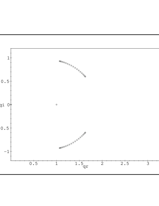
FIG. 3.: Zeros of $Z(S_{m},q,a)$ in the $q$ plane for $a=0.1$. For this and the other figures on zeros of $Z(S_{m},q,a)$, we use $m=19$, i.e., $n=42$. The axis labels are $qr\equiv Re(q)$ and $qi\equiv Im(q)$ here and in other $q$-plane plots.

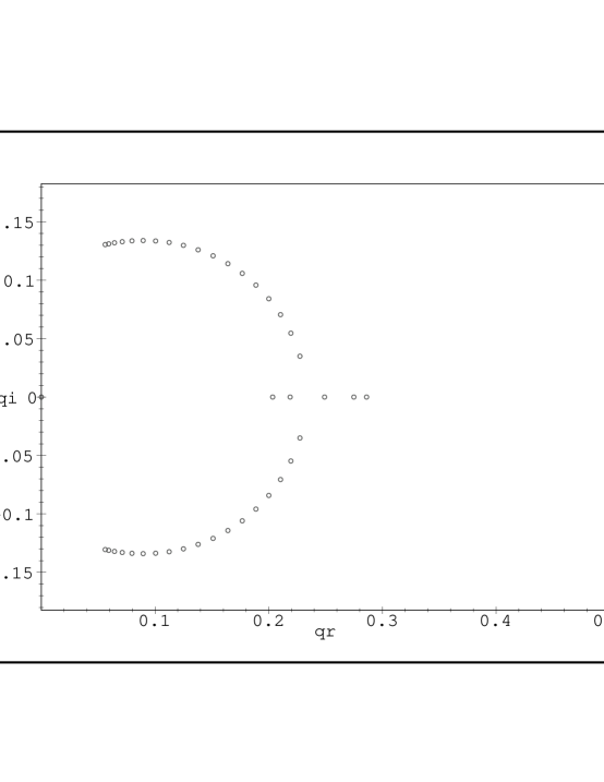
FIG. 4.: Same as Fig. 3 for $a=0.9$.

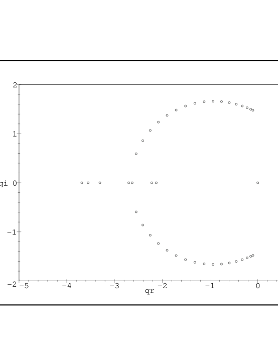
FIG. 5.: Same as Fig. 3 for $a=2$.

One can also consider negative real values of $a$, which correspond to complex temperature. As $a$ decreases from 0 through real values, ${\cal B}_{q}$ forms arcs, as was the case when $a$ increased from 0; these arcs have endpoints at the branch point singularities of $\lambda_{S,j}$ and elongate as $a$ moves downward in the range $-1<a<0$. As $a$ reaches $-1$, these arcs touch the positive real $q$ axis at the point $q=2$ and join to form a single self-conjugate arc (with endpoints at $4\pm 4i$), but as $a$ decreases below $-1$, the arcs retract from the real axis to form two c.c. parts again. It is straightforward to consider complex values of $a$ also, but we shall restrict ourselves to real $a$ here.

B ${\cal B}_{u}(\{S\})$ for fixed $q$

For our analysis of ${\cal B}_{u}(\{S\})$ we start with large $q$. Here ${\cal B}_{u}$ consists of a self-conjugate arc that crosses the real $u$ axis, together with a complex-conjugate pair of arcs that are concave toward the real $u$ axis. As $q\to\infty$, these arcs all shrink and move in toward the origin of the $u$ plane. This limit thus commutes with the result of taking $q\to\infty$ first before taking $n\to\infty$; in this case,

$$\lambda_{S,1}=q^{2}+3vq+O(1)\ ,\quad\lambda_{S,2}=v^{2}(1+v)+O\Bigl{(}\frac{1}{q}\Bigr{)}\quad{\rm as}\quad q\to\infty$$ (92)

so that the degeneracy equation $|\lambda_{S,1}|=|\lambda_{S,2}|$ has no solution for $q\to\infty$. In Fig. 6 we show the complex-temperature zeros of $Z$ for a typical value, $q=10$, calculated for $L_{x}=m+1=20$, i.e., $n=42$. With this large a value of $n$, these zeros occur close to the asymptotic locus ${\cal B}_{u}$ and give an adequate indication of its location. The self-conjugate arc crosses the real $u$ axis at $u\simeq-0.3954$ where the quantity $T_{S12}$ in eq. (71) vanishes, so that $|\lambda_{S,1}|=|\lambda_{S,2}|$. The endpoints of this arc occur at two of the zeros of the square root in eq. (70), viz., $u\simeq-0.2937\pm 0.3870i$. The two c.c. arcs have their endpoints at the four other zeros of this square root, at $u\simeq-0.1361\pm 0.14245i$ and $u\simeq 0.1178\pm 0.8130i$.

As $q$ decreases, the endpoints of the self-conjugate arc retract toward the real axis, it curls over to be more concave to the right, and the point at which it crosses the real axis moves to the left. For example, for $q=4$, the self-conjugate arc crosses the real axis at $u=-1$ and has its endpoints at $q\simeq-0.4341\pm 1.3178i$, and the c.c arcs extend between endpoints at $q\simeq-0.3697\pm 0.2394i$ and $q\simeq 0.1711\pm 0.1593i$. For $q=3$ (see Fig. 7), the self-conjugate arc crosses the real axis at $u\simeq-1.2767$ and has endpoints at $q\simeq-0.5498\pm 0.2489i$, and the c.c. arcs extend between $q\simeq-0.0839\pm 2.0177i$ and $0.1892\pm 0.1974i$, passing through the points $u,u^{*}=e^{\pm 2\pi i/3}$. These results for $q=3$ and 4 have interesting implications that we shall discuss further below. The changes in ${\cal B}_{u}$ as $q$ decreases further toward $q=2$ are illustrated in Fig. 8 where we show the $q=2.5$ case. The self-conjugate arc crosses the real axis at $u\simeq-1.323$ and has endpoints at $u\simeq-0.7249\pm 0.2083i$ while the c.c pairs of arcs have endpoints at $q\simeq 0.2006\pm 0.2272i$ and $q\simeq 0.56505\pm 2.4351i$.

For $q=2$ (Fig. 9), the quartic polynomial in the square root of eq. (70) factorizes into a quadratic polynomial times $(v+2)^{2}$, yielding the result (90). Correspondingly, the self-conjugate arc disappears, and the locus ${\cal B}$ consists of two complex-conjugate arcs located in the half-plane $Re(q)\geq 0$, and touching the imaginary axis at $u=\pm i$. This locus is invariant under the inversion map $u\to 1/u$. The upper arc extends from the left endpoint at $u_{e1}\simeq 0.2138+0.2720i$ through $u=i$ to a right endpoint at $u_{e2}=1/u_{e1}^{*}\simeq 1.78615-2.2720i$, and so forth for the c.c. arc. As we have discussed before in the context of ${\cal B}_{q}$ [32] (see also [59, 60]), these endpoints are the zeros of the square root in (90) where there are finite branch point singularities in $\lambda_{S,1}$. There is also a discrete zero of $Z$ at the point $u=-1$ with multiplicity scaling proportional to the lattice size. As we proved in a previous theorem (Theorem 6 of Ref. [55]), this zero arises for the Ising model on a lattice with odd coordination number; in the present case, all of the vertices of the strip $S$ except those on the four end-corners have $\Delta=3$.

Because of the unphysical nature of the Potts/random cluster model for $q<2$, we shall not discuss this range except to mention another example of the noncommutativity (19) at $q=0$. If one first sets $q=0$ and calculates $Z$, then, since $Z=0$ identically, the set of zeros of $Z$ is vacuous. However, if one takes the limit $n\to\infty$, calculates the accumulation set ${\cal B}_{u}$, and then takes the limit $q\to 0$, one finds that $\lim_{q\to 1}{\cal B}_{u}$ is not the empty set. This is clear from the fact that in the limit $q\to 0$

$$\lambda_{S,(1,2);q=0}=\frac{v^{2}}{2}\Bigl{[}v+4\pm(v^{2}+4v+12)^{1/2}\Bigr{]}$$ (93)

so that the degeneracy equation $|\lambda_{S,1;q=0}|=|\lambda_{S,2;q=0}|$ has a nontrivial solution, namely the section of the the circular arc in the $Re(u)<0$ half-plane

$${\cal B}_{u}:\quad u=\frac{1}{3}e^{i(\pi\pm\theta)}\ ,\quad 0\leq\theta\leq arctan(2\sqrt{2})$$ (94)

which crosses the real axis at $u=-1/3$ (i.e., $v=-4$) and has endpoints at $u=(-1\pm 2\sqrt{2}i)/9$.

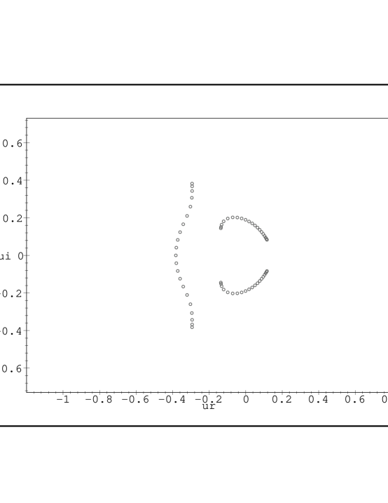
FIG. 6.: Zeros of $Z(S_{m},q,a)$ in the $u$ plane for $q=10$ and $m=19$ ($n=42$). The axis labels are $ur\equiv Re(u)$ and $ui\equiv Im(u)$ here and in other $u$-plane plots.

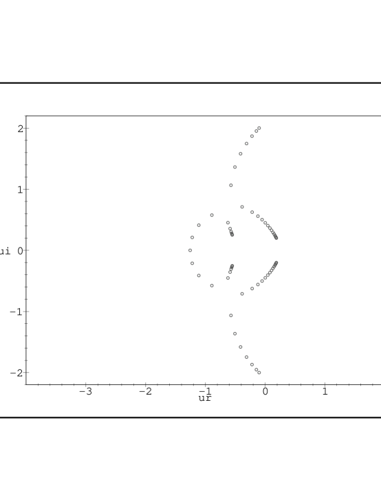
FIG. 7.: Same as Fig. 6 for $q=3$.

FIG. 8.: Same as Fig. 6 for $q=2.5$.

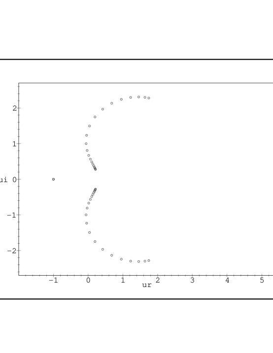
FIG. 9.: Same as Fig. 6 for $q=2$.

VI Cyclic and Möbius Ladder Graphs

A Results for $Z$

By either using an iterative application of the deletion-contraction theorem for Tutte polynomials and converting the result to $Z$, or by using a transfer matrix method (in which one starts with a $q^{2}\times q^{2}$ transfer matrix and generalizes to arbitrary $q$), one can calculate the partition function for the cyclic and Möbius ladder graphs of arbitrary length, $Z(G,q,v)$, $G=L_{m},\ ML_{m}$. We have used both methods as checks on the calculation. Our results have the general form (29) with $N_{\lambda}=6$ and are

$$Z(L_{m},q,v)=\sum_{j=1}^{6}c_{L,j}(\lambda_{L,j})^{m}$$ (95)

and

$$Z(ML_{m},q,v)=\sum_{j=1}^{6}c_{ML,j}(\lambda_{ML,j})^{m}$$ (96)

where

$$\lambda_{ML,j}=\lambda_{L,j}\ ,\quad j=1,...,6$$ (97)

$$\lambda_{L,1}=v^{2}$$ (98)

$$\lambda_{L,2}=v(v+q)$$ (99)

$$\lambda_{L,(3,4)}=\frac{v}{2}\Bigl{[}q+v(v+4)\pm(v^{4}+4v^{3}+12v^{2}-2qv^{2}+4qv+q^{2})^{1/2}\Bigr{]}$$ (100)

and

$$\lambda_{L,5}=\lambda_{S,1}\ ,\quad\lambda_{L,6}=\lambda_{S,2}$$ (101)

where $\lambda_{S,j}$, $j=1,2$ for the open ladder were given above in eq. (70). We note that $\lambda_{L,3}\lambda_{L,4}=(1+v)(q+v)v^{3}$ and $\lambda_{L,5}\lambda_{L,6}=(1+v)(q+v)^{2}v^{2}$. Chromatic and Tutte polynomials for recursive families of graphs obey certain recursion relations [22, 34]. In terms of the equivalent Tutte polynomial, given in the appendix, the results (95) and (96) agree with a recursion relation given in Ref. [22] (see also [23]).

The coefficient functions for the cyclic and Möbius ladders are

$$c_{L,1}=q^{2}-3q+1$$ (102)

$$c_{L,2}=c_{L,3}=c_{L,4}=c_{ML,3}=c_{ML,4}=q-1$$ (103)

$$c_{L,5}=c_{L,6}=c_{ML,5}=c_{ML,6}=1$$ (104)

$$c_{ML,1}=-1$$ (105)

$$c_{ML,2}=1-q\ .$$ (106)

Because of the equalities $c_{G,3}=c_{G,4}$ and $c_{G,5}=c_{G,6}$ for $G=L$ and for $G=ML$, we can again apply the theorem on symmetric polynomial functions of roots of algebraic equations [61] to confirm that, although the $\lambda_{G,j}$’s for nonpolynomial algebraic functions of $q$ and $v$ for $j=3,4,5,6$, $Z(G_{m},q,v)$ is a polynomial function of these variables $q$ and $v$, as it must be by (8).

B Special values and expansions of $\lambda$’s

We discuss some special cases. First, for the zero-temperature Potts antiferromagnet, i.e. the case $a=0$ ($v=-1$), the partition functions $Z(L_{m},q,v)$ and $Z(ML_{m},q,v)$ reduce, in accordance with the general result (10), to the respective chromatic polynomials $P(L_{m},q)$ and $P(ML_{m},q)$ calculated in [22]. In this special case, we have $\lambda_{L,1}=1$, $\lambda_{L,2}=1-q$, and (for an appropriate choice of sign of terms of the form $\sqrt{(q-3)^{2}}$ and $\sqrt{(D_{4})^{2}}$  ) $\lambda_{L,3}=3-q$, $\lambda_{L,4}=0$, $\lambda_{L,5}=D_{4}=q^{2}-3q+3$, and $\lambda_{L,6}=0$. For the infinite-temperature value $a=1$, we have $\lambda_{L,j}=0$ for $j=1,2,3,4,6$, while $\lambda_{L,5}=q^{2}$, so that $Z(G,q,a=1)=q^{2m}=q^{n}$ for $G=L_{m},\ ML_{m}$, in accord with the general result (14).

At $q=0$, besides the $q$-independent $\lambda_{L,1}$, we find

$$\lambda_{L,2}=(a-1)^{2}$$ (107)

$$\lambda_{L,3}=\lambda_{L,5}=\frac{1}{2}(a-1)^{2}\biggl{[}a+3+(a^{2}+2a+9)^{1/2}\biggr{]}$$ (108)

$$\lambda_{L,4}=\lambda_{L,6}=\frac{1}{2}(a-1)^{2}\biggl{[}a+3-(a^{2}+2a+9)^{1/2}\biggr{]}\ .$$ (109)

Since $\lambda_{L,3}$ and $\lambda_{L,5}$ are leading and are degenerate at this point, it follows that

$$q=0\quad{\rm is\ on}\quad{\cal B}_{q}(\{L\})\quad\forall\ a\ .$$ (110)

At $q=1$, $c_{L,j}=0$ for $j=2,3,4$ so that the corresponding $\lambda_{L,j}$, $j=2,3,4$, do not contribute to $Z$. Further, $c_{L,1}=-1=-c_{L,j}$, $j=5,6$ and $\lambda_{L,1}=\lambda_{L,6}=(a-1)^{2}$ so that the contributions of these terms cancel in $Z$, leaving only the contribution of $\lambda_{L,5}$: $Z(L_{m},q=1,a)=(\lambda_{L,5})^{m}=a^{3m}$, in agreement with the general formula (13).

In order to study the zero-temperature critical point in the ferromagnetic case and also the properties of the complex-temperature phase diagram, we calculate the $\lambda_{G,j,u}$’s corresponding to the $\lambda_{G,j}$’s, using eq. (38). This gives $\lambda_{L,1,u}=u(1-u)^{2}$, $\lambda_{L,2,u}=u(1-u)[1+(q-1)u)]$, and so forth for the others. In the vicinity of the point $u=0$ one has

$$\lambda_{L,1,u}=u-2u^{2}+u^{3}$$ (111)

$$\lambda_{L,2,u}=u+(q-2)u^{2}+(1-q)u^{3}$$ (112)

and the Taylor series expansions

$$\lambda_{L,3,u}=1-u^{2}+2(q-2)u^{3}+O(u^{4})$$ (113)

$$\lambda_{L,4,u}=u+(q-4)u^{2}+(7-3q)u^{3}+O(u^{4})$$ (114)

$$\lambda_{L,5,u}=1+(q-1)u^{2}\Bigl{[}1+4u+O(u^{2})\Bigr{]}$$ (115)

$$\lambda_{L,6,u}=u+2(q-2)u^{2}+(q^{2}-7q+7)u^{3}+O(u^{4})\ .$$ (116)

Hence, at $u=0$, $\lambda_{L,3,u}$ and $\lambda_{L,5,u}$ are dominant and $|\lambda_{L,3,u}|=|\lambda_{L,5,u}|$, so that the point $u=0$ is on ${\cal B}_{u}$ for any $q\neq 0,1$, where the noncommutativity (19) occurs. For $q>0$, $\lambda_{L,5,u}$ is dominant on the real $u$ axis in the vicinity of $u=0$ and hence in the PM and O phases that can be reached by analytic continuation therefrom, while the term $\lambda_{L,3,r}$ is dominant on the imaginary $u$ axis in the neighborhood of the origin, and hence in the O phases that can be reached by analytic continuation from this neighborhood.

To determine the angles at which the branches of ${\cal B}_{u}$ cross each other at $u=0$, we write $u$ in polar coordinates as $u=re^{i\theta}$, expand the degeneracy equation $|\lambda_{L,3,u}|=|\lambda_{L,5,u}|$, for small $r$, and obtain $qr^{2}\cos(2\theta)=0$, which implies that (for $q\neq 0,1$) in the limit as $r=|u|\to 0$,

$$\theta=\frac{(2j+1)\pi}{4}\ ,\quad j=0,1,2,3$$ (117)

or equivalently, $\theta=\pm\pi/4$ and $\theta=\pm 3\pi/4$. Hence there are four branches of ${\cal B}_{u}$ intersecting at $u=0$ and these branches cross at right angles. The point $u=0$ is thus a multiple point on the algebraic curve ${\cal B}_{u}$, in the technical terminology of algebraic geometry (i.e., a point where several branches of an algebraic curve cross [62]).

In order to investigate how these crossings depend on $L_{y}$, we have calculated $Z$ for the cyclic strip graph of the square lattice with the next larger width, $L_{y}=3$. Since the $T=0$ critical point for the Potts ferromagnet is present for each $q\neq 0,1$, it suffices to do this calculation for the simple $q=2$ Ising case (bearing in mind the noncommutativity that applies at special values $q_{s}$ as discussed above). We find that there are two $\lambda_{j}$’s that are dominant near $u=0$, and the small–$u$ expansion of the degeneracy equation yields the condition $r^{3}\cos(3\theta)=0$, so that there are six curves on ${\cal B}_{u}$ crossing $u=0$, at the angles $\theta=(2j+1)\pi/6$, $j=0,1,...,5$. This leads to the generalization that for the cyclic strip graph of the square lattice with width $L_{y}$, there are $2L_{y}$ curves on ${\cal B}_{u}$ that cross each other at $u=0$, at the angles $\theta=(2j+1)\pi/(2L_{y})$, $j=0,1,...,2L_{y}-1$. This inference implies, in turn, that in the limit $L_{y}\to\infty$, an infinite number of curves on ${\cal B}_{u}$ intersect at $u=0$, and the complex-temperature (Fisher) zeros become dense in the neighborhood of this point. Since the origin of this phenomenon is not dependent in detail on the lattice type, one would also infer that it occurs for infinite-length width $L_{y}$ cyclic strips of other lattices.

For $q=0,1$ the (23) occurs, with $({\cal B}_{u})_{nq}=\emptyset$ by eqs. (25) and (26), but $({\cal B}_{u})_{qn}\neq\emptyset$. While ${\cal B}_{u}$ is compact for $q\neq 2$, it is noncompact for $q=2$, where the symmetry (27) holds.

Our exact calculations yield the following general result

$${\cal B}(\{L\})={\cal B}(\{ML\})\ .$$ (118)

This is in accord with the conclusion that the singular locus is the same for an infinite-length finite-width strip graph for given transverse boundary conditions, independent of the longitudinal boundary condition. This generalizes our previous finding that ${\cal B}_{q}$ was independent of the longitudinal boundary conditions for the case $a=0$ [37, 41, 43]. In the present case, the result (118) follows immediately because $Z(L_{m},q,v)$ and $Z(ML_{m},q,v)$ involve the same $\lambda_{j}$’s. We note that this is a sufficient, but not necessary condition for the loci to be the same for a given family of graphs when one changes the longitudinal boundary conditions; it may be recalled that for the $T=0$ Potts antiferromagnet on the width $L_{y}=3$ strip of the square [42] with periodic transverse boundary conditions, when one changed from periodic to twisted periodic longitudinal boundary conditions, i.e. toroidal to Klein bottle topology, three of the $N_{\lambda}=8$ terms were absent. However, since none of these was a dominant term anywhere, the locus ${\cal B}_{q}$ was the same for either toroidal or Klein bottle boundary conditions. From our calculation of the chromatic polynomial for the width $L_{y}=3$ strip of the triangular lattice with both free and periodic transverse boundary conditions and periodic and twisted periodic longitudinal boundary conditions [46] we found that a similar situation occured for the toroidal versus Klein bottle boundary conditions: six of the $N_{\lambda}=11$ terms in the toroidal case were absent in the Klein bottle case, but again none of these was dominant anywhere. Owing to the equality (118), we shall henceforth, for brevity of notation, refer to both ${\cal B}(\{L\})$ and ${\cal B}(\{ML\})$ as ${\cal B}(\{L\})$ and similarly for specific points on ${\cal B}$, such as $q_{c}(\{L\})=q_{c}(\{ML\})$, etc.

C ${\cal B}_{q}(\{L\})$ for fixed $a$

We find that ${\cal B}_{q}(\{L\})$ crosses the real $q$ axis at

$$q_{c}(\{L\})=(1-a)(a+2)\ .$$ (119)

This is the solution to the degeneracy equation of leading terms $|\lambda_{L,5}|=|\lambda_{L,3}|=|\lambda_{L,2}|$. As $a$ increases from 0 to 1, $q_{c}(\{L\})$ decreases monotonically from 2 to 0. From eq. (119) it follows that there are, in general, two values of $a$ that correspond to this value of $q$ on ${\cal B}(\{L\})$, viz.,

$$a_{c,\pm}(\{L\})=\frac{1}{2}[-1\pm\sqrt{9-4q}\ ]\ ,\quad i.e,\quad u_{c,\pm}(\{L\})=\frac{-1\pm\sqrt{9-4q}\ }{2(q-2)}\ .$$ (120)

D Antiferromagnetic Case, $T=0$

We start with the $T=0$ antiferromagnet, i.e. the case $a=0$. After initial studies in Refs. [22, 26, 28], the locus ${\cal B}$ was determined in Ref. [21]. As is shown in Fig. 3 of Ref. [21], ${\cal B}_{q}$ separates the $q$ plane into four regions, and $q_{c}(\{L\})=2.$ The outermost region is $R_{1}$, and includes the segments $2\leq q$ and $q<0$ on the real $q$ axis; in this region $\lambda_{L,5}$ is dominant. The innermost region, denoted $R_{3}$, includes the segment $0\leq q\leq 2$ on the real axis; in this region, the term $\lambda_{L,3}$ is dominant. In addition, there are two other complex-conjugate regions, $R_{2}$ and $R_{2}^{*}$, which touch the real axis at $q=q_{c}(\{L\})=2$ and stretch outward to triple points at

$$q_{L,trip.},\ q_{L,trip.}^{*}=2\pm\sqrt{2}\ i\ .$$ (121)

The part of ${\cal B}$ separating region $R_{3}$ from regions $R_{2}$, $R_{2}^{*}$ is the line segment $Re(q)=2$, $-\sqrt{2}\leq Im(q)\leq\sqrt{2}$. In regions $R_{2}$, $R_{2}^{*}$, $\lambda_{2}$ is dominant. At $q=2$ all four terms are degenerate (recall that for $a=0$, $\lambda_{L,4}=\lambda_{L,6}=0$). At the triple points $q_{L,trip.}$, there are three degenerate leading terms, with $|\lambda_{L,5}|=|\lambda_{L,3}|=|\lambda_{L,2}|$. All four regions are contiguous at $q_{c}(\{L\})$.

E Antiferromagnet Case for $T>0$

We proceed to consider the regions in the $q$ plane for the Potts antiferromagnet at arbitrary nonzero temperature, i.e. the range $0<a\leq 1$. The zeros of $Z$ in the $q$ plane are shown for several values of $a$ in the figures. In this range $0<a<1$ we find a number of general features. As was true at $T=0$, ${\cal B}_{q}$ continues to separate the $q$ plane into different regions and, as indicated in eq. (110) and (119), this locus crosses the real axis at $q=0$ and $q_{c}(\{L\})$. ${\cal B}_{q}$ consists of a single connected component made up of several curves. Commenting on the regions in the $q$ plane, starting for $a$ near 0, we note that again the region $R_{1}$ is the outermost, and includes the semi-infinite line segment on the real axis $q>q_{c}(\{L\})$ and $q<0$; region $R_{3}$ is the innermost region, and includes the line segment $0\leq q\leq q_{c}(\{L\})$. The complex-conjugate regions $R_{2}$ and $R_{2}^{*}$ extend upward and downward from $q_{c}(\{L\})$ to triple points. As $a$ increases, the complex-conjugate regions $R_{2}$ and $R_{2}^{*}$ are reduced in size. As is evident in the figures, as $a$ increases from 0 to 1, the locus ${\cal B}_{q}$ contracts toward the origin, $q=0$ and in the limit as $a\to 1$, it degenerates to a point at $q=0$. This also describes the general behavior of the partition function zeros themselves. That is, for finite graphs, there are no isolated partition function zeros whose moduli remains large as $a\to 1$. This is clear from continuity arguments in this limit, given eq. (14).

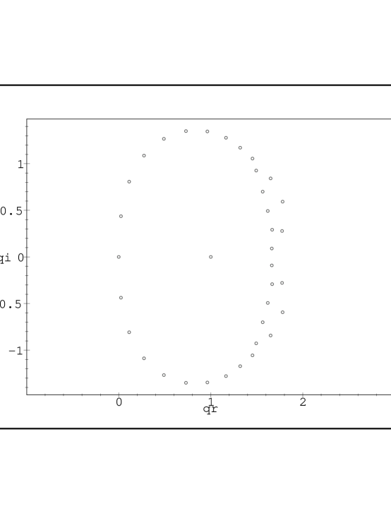
FIG. 10.: Zeros of $Z(L_{m},q,a)$ in the $q$ plane for $a=0.25$ and $m=18$ ($n=36$).

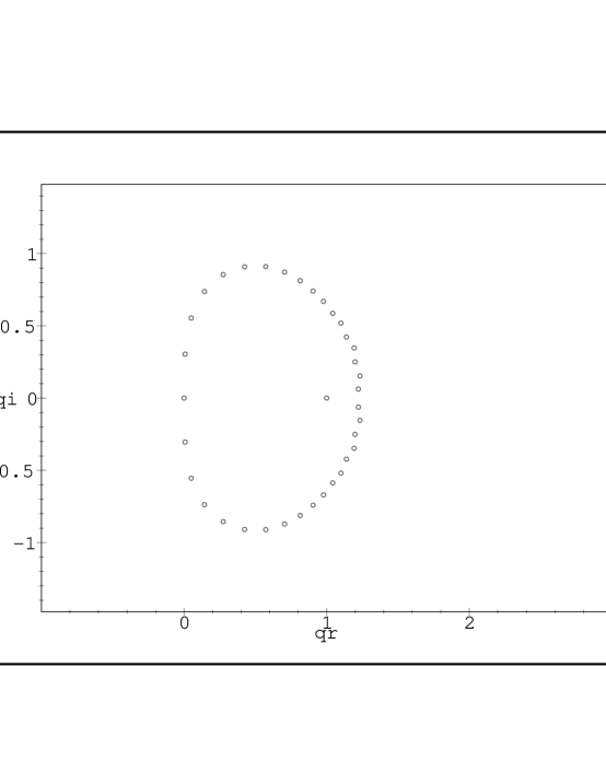
FIG. 11.: Same as Fig. 10 for $a=0.5$.

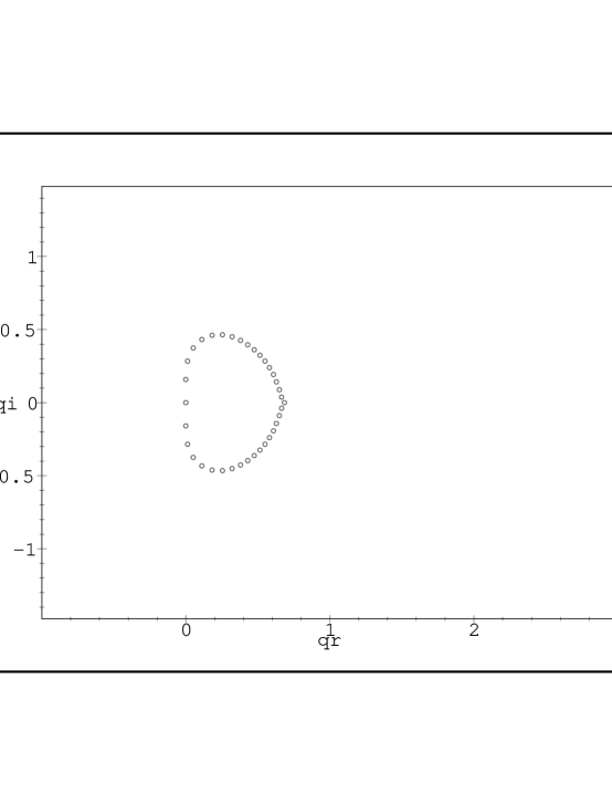
FIG. 12.: Same as Fig. 10 for $a=0.75$.

F Ferromagnetic Case

In Fig. 13 we show the zeros of $Z$ for a typical ferromagnetic values, $a=2$. We find the following general features of ${\cal B}_{q}$ for the ferromagnetic Potts model for the full range of temperature. The locus ${\cal B}_{q}$ contains a heart-shaped figure and a finite line segment on the negative real $q$ axis. The line segment occurs because the expression in the square roots in $\lambda_{L,5}$ and $\lambda_{L,6}$, given as $R_{S12}$ in eq. (72), is negative in an interval of the negative real axis, yielding a pure imaginary square root so that, given that $T_{S12}$ is real, $|\lambda_{L,5}|=|\lambda_{L,6}|$. For example, for the case shown in Fig. 13, $R_{S12}<0$ for $-3.73<q<-2.10$; within this interval, $|\lambda_{L,5}|=|\lambda_{L,6}|$ are leading for $-3.73<q<3.35$, thereby producing the line segment. (For the remaining part of the interval, $-3.35<q<-2.10$, these eigenvalues have smaller magnitudes than $|\lambda_{L,3}|$ and hence do not determine the locus ${\cal B}_{q}$.) The size of the heart-shaped boundary increases as $a$ increases. Since $q_{c}(\{L\})$, given in eq. (119), is negative, ${\cal B}_{q}$ does not intersect the positive real $q$ axis. As was true for the Potts AF, in the region exterior to ${\cal B}_{q}$ in the $q$ plane, the dominant $\lambda_{j}$ is $\lambda_{L,5}$, so that the (reduced) free energy is

$$f=\frac{1}{2}\ln\lambda_{L,5}=\frac{1}{2}\ln\lambda_{S,1}$$ (122)

where $\lambda_{S,1}$ was given in eq. (70). For the range $q>2$ where this system has acceptable physical behavior, the above expression for the free energy holds for all (physical) temperatures. We shall discuss the thermodynamics further below. In the region interior to ${\cal B}_{q}$, $\lambda_{L,3}$ is dominant, so $|e^{f}|=|\lambda_{L,3}|^{1/2}$.

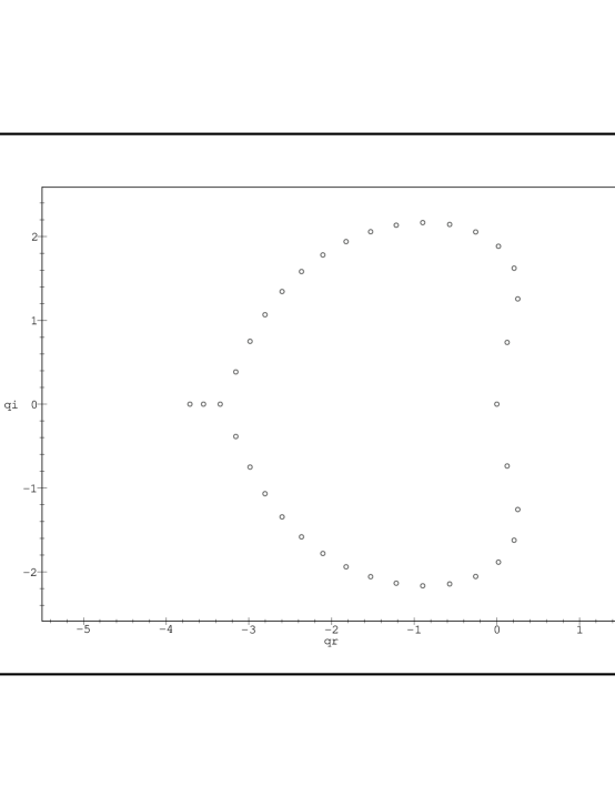
FIG. 13.: Zeros of $Z(L_{m},q,a)$ in $q$ for $a=2$ and $m=18$ ($n=36$).

G ${\cal B}_{q}$ for $a<0$

We briefly comment on ${\cal B}_{q}$ for negative real values of $a$, which correspond to complex temperature (as well as complex values of $a$ not considered here). For the interval

$$-\frac{1}{2}<a<0$$ (123)

the regions $R_{2}$ and $R_{2}^{*}$, which were separate, although contiguous at $q=q_{c}(\{L\})$, for $a$ in the interval $0\leq a<1$, now merge to form one region, which we shall call $R_{22*}$ to indicate this merger. In this region, $\lambda_{L,2}$ is dominant. The $R_{22*}-R_{1}$ boundary is determined by the degeneracy equation $|\lambda_{L,2}|=|\lambda_{L,5}|$ and crosses the real axis at $q_{c}(\{L\})$. The point at which the $R_{3}-R_{22*}$ boundary crosses the real axis is determined by the relevant root of the threefold degeneracy equation $|\lambda_{L,3}|=|\lambda_{L,2}|=|\lambda_{L,5}|$, and is

$$q_{b\ell}=2(1-a)\quad{\rm for}-\frac{1}{2}<a<0\ .$$ (124)

The width of the merged $R_{22^{*}}$ region on the real axis is thus $(-a)(1-a)$ for this range of $a$. As $a$ decreases in the interval (123), $q_{b\ell}$ and $q_{c}$ both increase above 2. When $a$ decreases through the value $a=-1/2$, at which point $q_{b\ell}=9/4$, the square root in $\lambda_{L,3}$ becomes complex. Viewed the other way, solving eq. (124) for $a$ gives

$$a_{b\pm}=\frac{1}{2}\Bigl{[}-1\pm\sqrt{9-4q}\ \Bigr{]}\ .$$ (125)

We are interested in the larger solution, $a_{b+}$. When $q$ increases through 9/4, corresponding to $a_{b+}=-1/2$, the square root becomes complex, and there is no longer a real solution for $a_{b\pm}$. The region diagram changes qualitatively for $a<-1/2$. The illustrative case $a=-1$ is shown in Fig. 14. Note that $Z(L_{m},q,a=-1)$ has an overall factor $q(q-2)$. Here ${\cal B}_{q}$ crosses the real $q$ axis at $q=2$ and $q=q_{c}=4$ as well as at $q=0$. The crossing at $q=4$ is a multiple point on the algebraic curve. Other interesting changes occur for larger negative values of $a$, but we shall forgo discussing them to proceed to the physical range of real $a\geq 1$.

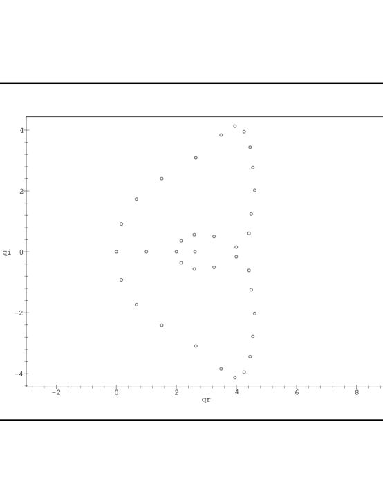
FIG. 14.: Zeros of $Z(L_{m},q,a)$ in $q$ for $a=-1$ and $m=18$.

H Thermodynamics of the Potts Model on the $L_{y}=2$ Strip

1 $q\geq 2$

In this section we first restrict to the range $q\geq 2$ where the Potts/random cluster model has physical behavior for both the ferromagnetic and antiferromagnetic cases, and then consider the behavior for $0<q<2$. For $q\geq 2$, the free energy is given for all temperatures by (122). It is straightforward to obtain the internal energy $U$ and specific heat $C$ from this free energy; since the expressions are somewhat complicated we do not list them here but instead concentrate on their high- and low-temperature expansions and general features, as compared with those for the $L_{y}=1$ case. The high-temperature expansion of $U$ is

$$U=-\frac{3J}{2q}\biggl{[}1+\frac{(q-1)}{q}K+O(K^{2})\biggr{]}\ .$$ (126)

The expression in brackets is the same as that for the $L_{y}=1$ strip up to and including the $K^{2}$ term. For the specific heat we have

$$C=\frac{3k_{B}(q-1)K^{2}}{2q^{2}}\biggl{[}1+\frac{(q-2)}{q}K+O(K^{2})\biggr{]}$$ (127)

(here the order $K^{2}$ term differs from that for $L_{y}=1$.) The low-temperature expansions for the ferromagnet ($K\to\infty$) and antiferromagnet ($K\to-\infty$) are

$$U=J\Biggl{[}-\frac{3}{2}+(q-1)e^{-2K}\biggl{[}1+6e^{-K}+7(q-1)e^{-2K}+O(e^{-3K})\biggr{]}\Biggr{]}\quad{\rm as}\quad K\to\infty$$ (128)

and

$$U=\frac{(-J)e^{K}}{2(D_{4})^{2}}\biggl{[}t_{1}+t_{2}e^{K}+O(e^{2K})\biggr{]}\quad{\rm as}\quad K\to-\infty$$ (129)

where $D_{4}=q^{2}-3q+3$ was given in (85) and

$$t_{1}=(q-2)(3q^{2}-9q+8)$$ (130)

$$t_{2}=-\frac{(3q^{6}-42q^{5}+211q^{4}-532q^{3}+734q^{2}-534q+162)}{(D_{4})^{2}}$$ (131)

$$C=2k_{B}K^{2}(q-1)e^{-2K}\biggl{[}1+9e^{-K}+14(q-1)e^{-2K}+O(e^{-3K})\biggr{]}\quad{\rm as}\quad K\to\infty$$ (132)

and

$$C=\frac{k_{B}K^{2}e^{K}}{2(D_{4})^{2}}\biggl{[}t_{1}+2t_{2}e^{K}+O(e^{2K})\biggr{]}\ .\quad{\rm as}\quad K\to-\infty$$ (133)

Again, we observe that for the Ising case $q=2$, these expansions satisfy the symmetry relations (17) and (18). (In passing, we mention the generalization of the first term in eq. (128) to arbitrary $L_{y}$: in the $T=0$ limit of the Potts ferromagnet,

$$U=-\frac{\Delta_{ave}J}{2}=-2\Bigl{[}1-\frac{1}{2L_{y}}\Bigr{]}J\ .$$ (134)

We show plots of $C$ (with $k_{B}=1$) for the ferromagnetic and antiferromagnetic Potts model on the $L_{y}=2$ strip (in the $L_{x}\to\infty$ limit) in Figs. 15 and 16. As was true for $L_{y}=1$, in the antiferromagnetic case, $C$ is a decreasing function of $q$ for all finite temperature, while in the ferromagnetic case, $C$ increases (decreases) with $q$ at low (high) temperatures and has a maximum that increases with $q$. For a fixed $q$, by comparing the previous plots of the specific heat on the line ($L_{y}=1$ case) with the corresponding plots for the $L_{y}=2$ strip, for the ferromagnet, and for the antiferromagnet, one can see quantitatively how the behavior of this function changes as $L_{y}$ increases.

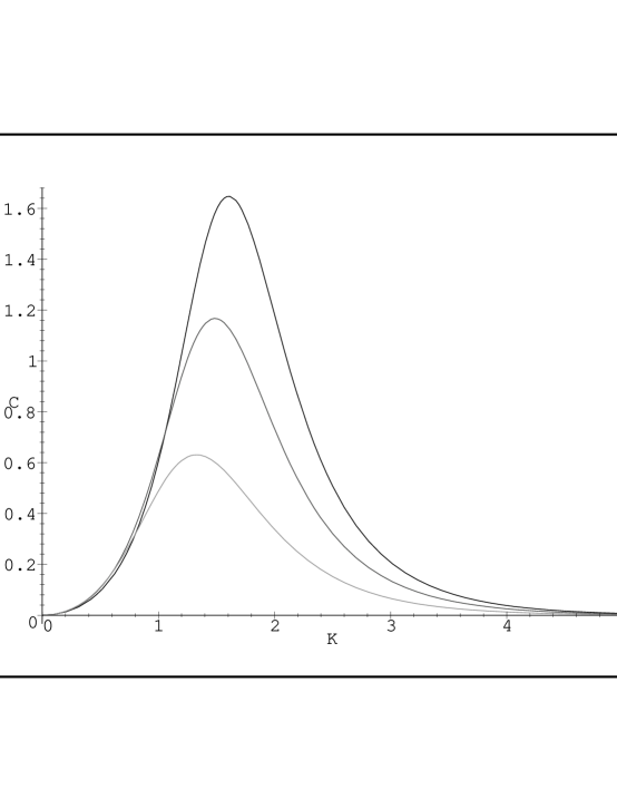
FIG. 15.: Specific heat for the Potts ferromagnet on the infinite-length, width $L_{y}=2$ strip (ladder) as a function of $K=J/(k_{B}T)$. Going from bottom to top in order of the heights of the maxima, the curves are for $q=2,3,4$.

FIG. 16.: Specific heat for the Potts antiferromagnet on the infinite-length, width $L_{y}=2$ strip (ladder) as a function of $-K=-J/(k_{B}T)$. Going downward in order of the heights of the maxima, the curves are for $q=2,3,4$.

For both the $L_{y}=1$ and $L_{y}=2$ strips, we observe that the exponential zero in the specific heat as $T\to 0$ for both the ferromagnetic and antiferromagnetic cases is $C\sim(q-1)K^{2}e^{-L_{y}|K|}$. For comparative purposes we have also calculated the partition function, free energy, and these thermodynamic functions for the Ising model on the strip with the next larger width, $L_{y}=3$. We find that the above dependence on $L_{y}$ is again exhibited, namely $C\sim K^{2}e^{-3|K|}$.

In view of the fact that the Potts ferromagnet has a zero-temperature critical point for the infinite-length, finite-width strip graphs of the square lattice (as does the Potts antiferromagnet in the $q=2$ case where it is equivalent to the ferromagnet on these graphs), it is of interest to investigate the dependence of the singularities in thermodynamic functions on the strip width $L_{y}$. As is typical for systems at their lower critical dimensionality, these are essential singularities. We have done this comparative study above for the specific heat. We next consider the (divergent) exponential singularities in the correlation length and the (uniform, zero-field) susceptibility (again, in the $q=2$ case, under the replacement $J\to-J$ and uniform $\to$ staggered, this subsumes the antiferromagnetic case). Define the ratio of the subleading eigenvalue divided by the leading eigenvalue of the transfer matrix for the strip graphs with periodic longitudinal boundary conditions considered here as $\rho_{L_{y}}$. Thus

$$\rho_{1}=\frac{\lambda_{C,2}}{\lambda_{C,1}}=\frac{v}{q+v}$$ (135)

and

$$\rho_{2}=\frac{\lambda_{L,3}}{\lambda_{L,5}}\ .$$ (136)

We have also calculated $\rho_{3}$ for the Ising case, but since it is a rather messy expression involving cube roots, we do not display it here. These ratios $\rho_{L_{y}}$ control the asymptotic decay of the spin-spin correlation function. For example, in the $n\to\infty$ limit, the spin-spin correlation function in the 1D case is given by $\langle\sigma_{r}\sigma_{r^{\prime}}\rangle\propto(\rho_{1})^{|r-r^{\prime}|}$. The correlation length can be written as

$$\xi=-\frac{1}{\ln\rho_{L_{y}}}\ .$$ (137)

For the 1D case, one knows that the correlation length has an exponential divergence as $T\to 0$: $\xi\sim q^{-1}e^{K}+O(1)$. For the $L_{y}=2$ strips we find

$$\xi\sim q^{-1}e^{2K}+O(e^{K})\ ,\quad{\rm as}\quad T\to 0\quad{\rm for}\quad\{G\}=\{L\}\ .$$ (138)

and for the Ising model on the width $L_{y}=3$ strip, we obtain $\xi\sim(1/2)e^{3K}+O(e^{2K})$. These results show that the exponential divergence in the correlation length is more rapid for larger width $L_{y}$ and are consistent with an inference that $\xi\sim q^{-1}e^{L_{y}K}+O(e^{(L_{y}-1)K})$ as $T\to 0$. The fact that the correlation length diverges more rapidly as $L_{y}$ increases is easily explained since this is due to the spin-spin interactions and the average effect of these interactions, as determined by the average coordination number, $\Delta_{ave}$ in eq. (16), increases as $L_{y}$ increases.

The zero-field susceptibility (per site) is well known for the 1D case: $\chi=\beta(1+\rho_{1})/(1-\rho_{1})$, which diverges as a function of $K$ like $\chi\sim Ke^{K}$ as $K\to\infty$. Our results for $L_{y}=2,3$ support the inference that $\chi\sim Ke^{L_{y}K}$ as $K\to\infty$. The more rapid divergence in $\chi$ as $L_{y}$ increases can be explained in the same way as was done for the correlation length.

The inferred $L_{y}$ dependence of the divergences in the correlation length $\xi$ and susceptibility $\chi$ at the zero-temperature critical point of the Potts ferromagnet dramatically illustrate the fact that the thermodynamic behavior of the model on this sequence of infinite-length, width $L_{y}$ strips of the square lattice is quite different, even in the limit $L_{y}\to\infty$, from the behavior of the model on the square lattice. In the latter case, the thermodynamic limit is $L_{x}\to\infty$, $L_{y}\to\infty$, with $\lim_{L_{x}\to\infty}L_{y}/L_{x}$ equal to a finite nonzero constant. For the strips, for any $L_{y}$ no matter how large, the ferromagnet is critical only at $T=0$, and as $T\to 0$ and $\xi\to\infty$, the strip acts as a one-dimensional system, since $lim_{L_{x}\to\infty}L_{y}/L_{x}=0$. In contrast, for the Potts model on the square lattice, the phase transition occurs at finite temperature, at the known value $K_{c}=\ln(1+\sqrt{q}\ )$. These studies of the thermodynamic behavior of the Potts model for general $q$ on $L_{y}\times\infty$ strips thus complement studies such as those on the approach to the thermodynamic limit of the Ising model on $L_{x}\times L_{y}$ rectangular regions, in which $L_{x}$ and $L_{y}$ both get large with a fixed finite ratio $L_{y}/L_{x}$ [63], and finite-size scaling analyses [64]. These differences are also evident in the behavior of ${\cal B}_{u}$; we have inferred above that as $L_{y}\to\infty$, there are an infinite number of curves on ${\cal B}_{u}$ that cross each other at the ferromagnetic zero-temperature critical point, $u=0$, so that the Fisher zeros become dense in the neighborhood of this point. This is quite different from the accumulation set of the Fisher zeros for the square lattice; although this is known exactly only for the Ising case, the existence of low-temperature expansions with a finite radius of convergence for the $q$-state Potts model is equivalent to the statement that the singular locus ${\cal B}_{u}$ does not pass through $u=0$.

In the case of the antiferromagnet, as we have shown [31], for $q$ values that are only moderately above the value of $q=3$ where the Potts antiferromagnet is critical on the square lattice, the ground state entropy of infinite-length, finite-width strips rapidly approaches its value for the square lattice. For the ($L_{x}\to\infty$ limit of the) $L_{y}=2$ strip, this is given by $S_{0}=(1/2)k_{B}\ln(q^{2}-3q+3)$, which is nonzero for $q>2$. The analytic expressions for the $L_{y}=3,4$ cases are given in [31]. This can be understood because the ground state entropy is a disorder quantity and, for $q>3$ is not associated with any large correlation length.

2 $0<q<2$: Phase Transition for Antiferromagnet

For the range $0<q<2$, our result for $a_{c,+}$ in eq. (120) shows that ${\cal B}$ crosses the positive real $a$ axis in the interval $0<a<1$, so that the Potts/random cluster antiferromagnet has a finite-temperature phase transition, at the temperature

$$T_{L,p}=\frac{J}{k_{B}\ln\Bigl{[}\frac{1}{2}\{-1+\sqrt{9-4q}\ \}\Bigr{]}}\ ,\quad 0<q<2$$ (139)

(where both $J$ and the log are negative, yielding a positive $T_{L,p}$). For $q=1$, it is understood that one takes $n\to\infty$ first and then $q\to 1$, i.e., that one uses the free energy $f_{qn}$. As $q$ decreases from 2 to 0, the phase transition temperature $T_{L,p}$ increases from 0 to infinity. In the high- and low-temperature phases, the free energy is given by eq. (122) and by $f=(1/2)\ln\lambda_{L,3}$, respectively. These results may be compared with the temperature $T_{p}$ in eq. (58) for the circuit graph. The same comments that we made in that case apply here; this result does not contradict the usual theorem that 1D (and quasi-1D) spin systems with short-range interactions do not have any finite-temperature phase transition because the phase transition here is intrinsically connected with unphysical behavior of the model in the low-temperature phase, including negative specific heat, negative partition function, and non-existence of an $n\to\infty$ limit for thermodynamic functions that is independent of boundary conditions. Indeed, the last pathology is obvious from the fact that for the $n\to\infty$ limit of the ladder graph with open longitudinal boundary conditions, the free energy is given by eq. (82) for all temperatures, the singular locus ${\cal B}$ does not cross the positive $a$ axis, and there is no such phase transition at finite temperature.

Evidently, the temperature value at which the phase transition takes place in the Potts/random cluster antiferromagnet on the infinite-length limits of both the circuit graph and the cyclic and Möbius $L_{y}=2$ strip graphs is determined by the respective formulas relating $q_{c}$ to $a$, eqs. (54) and (119). From the point of view of ${\cal B}_{q}$ in the $q$ plane, as we have discussed, we find, as a general feature, that in the antiferromagnetic case, as one increases $T$ from 0 to infinity, the value of $q_{c}(\{G\})$ for a given family $\{G\}$ decreases from its $T=0$ value to the origin, $q=0$. Correspondingly, for the $n\to\infty$ limit of a given family $\{G\}$ with periodic (or twisted periodic) longitudinal boundary conditions, the antiferromagnet will exhibit a finite-temperature phase transition at a temperature $T_{\{G\},p}$ for the range $0<q<q_{c}(\{G\})$:

$$\exists\ T_{\{G\},p}>0\quad{\rm for}\quad 0<q<q_{c}(\{G\})\ .$$ (140)

Thus, for example, for the $L_{y}=3$ square strip of the square lattice with cyclic or Möbius boundary conditions, for which we determined ${\cal B}_{q}$ for the $T=0$ antiferromagnet [37] and, in particular, $q_{c}(sq,L_{y}=3,cyc.)\simeq 2.33654$, it follows that the random cluster antiferromagnet has a finite-temperature phase transition for $0<q<q_{c}(sq,L_{y}=3,cyc.)$. Just as we have discussed above, at special integer values $q_{s}$ in the range $0<q<q_{c}(\{G\})$, it is understood that one takes the limit $n\to\infty$ first, and then $q\to q_{s}$ in calculating $f=f_{qn}$ and ${\cal B}_{u}=({\cal B}_{u})_{qn}$. Similarly, on the $L_{y}=2$ cyclic and Möbius triangular lattice strips, where we found that $q_{c}(tri,L_{y},cyc.)=3$ for $L_{y}=2$ [37] and $L_{y}=3$ [46], it follows that the Potts/random cluster antiferromagnet has a finite-temperature phase transition for $0<q<3$. In all cases, however, this transition involves unphysical aspects, among which is the non-existence of a unique $n\to\infty$ limit that is independent of boundary conditions.

I ${\cal B}_{u}(\{L\})$ for $q>4$

We next proceed to the slices of ${\cal B}$ in the plane defined by the temperature Boltzmann variable $u$, for given values of $q$, starting with large $q$. In the limit $q\to\infty$, the locus ${\cal B}_{u}$ is reduced to $\emptyset$. This follows because for large $q$, there is only a single dominant $\lambda_{j}$, namely

$$\lambda_{L,5}\sim q^{2}+3qv+O(1)\quad{\rm as}\quad q\to\infty\ .$$ (141)

Note that in this case, one gets the same result whether one takes $q\to\infty$ first and then $n=2m\to\infty$, or $n\to\infty$ and then $q\to\infty$, so that these limits commute as regards the determination of ${\cal B}_{u}$.

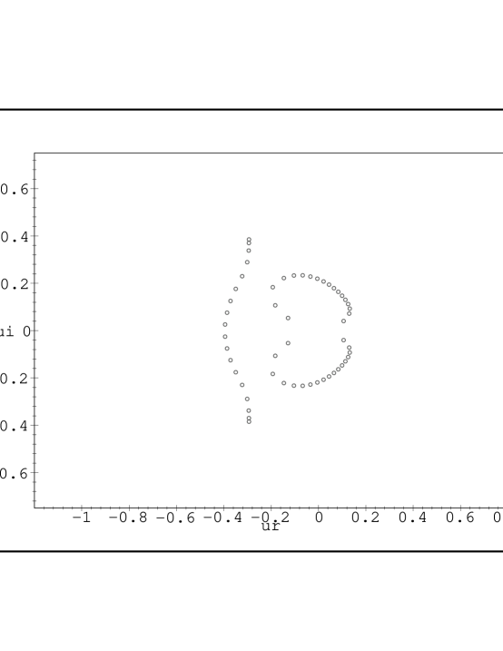
FIG. 17.: Zeros of $Z(L_{m},q,a)$ in the $u=1/a$ plane for $q=10$ and $m=18$ ($n=36$).

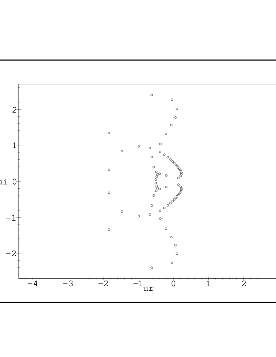
FIG. 18.: Zeros of $Z(L_{m},q,a)$ in the $u=1/a$ plane for $q=3$ and $m=24$ ($n=48$).

In the large–$q$ region we find that the locus ${\cal B}_{u}$ consists of two complex-conjugate curves that pass through $u=0$ at the angles (117), hence intersecting at right angles and forming a distorted figure-8, together with a separate self-conjugate arc. Thus, ${\cal B}_{u}$ is comprised of two disconnected parts. For real $q$, the degeneracies in magnitude among leading terms are $|\lambda_{L,3,u}|=|\lambda_{L,5,u}|$ at $u=0$ and $|\lambda_{L,5,u}|=|\lambda_{L,6,u}|$ at the point on the negative real axis where $T_{S12}=0$. As a typical illustration of ${\cal B}_{u}$ for the large-$q$ region, we show the complex-temperature zeros for $q=10$ calculated for $m=18$, i.e., $n=2m=36$, in Fig. 17. It is instructive to compare this plot with the analogous plot for the open strip with $q=10$ given above in Fig. 6. The self-conjugate arc is the same in the two plots, crossing the real $u$ axis at $u\simeq-0.3954$, where $T_{S12}=0$ and having endpoints at two of the zeros of the expression in the square root in $\lambda_{L,j}$, $j=5,6$, which are identical to $\lambda_{S,j}$, $j=1,2$ in eq. (70). A notable difference between the locus ${\cal B}_{u}$ for the cyclic or Möbius ladder and the analogous locus for the open square strip is that while the latter does not separate the $u$ plane into different regions, the former does. Specifically, there are three regions: the physical PM phase occupying the interval $0\leq u\leq\infty$ and its maximal analytic continuation, together with an $O_{1}$ phase in the interior of the upper curve and its complex-conjugate phase $O_{1}^{*}$. As is evident in the figure, the density of zeros on the curves decreases strongly as $u$ approaches the multiple point at $u=0$. In the PM phase $\lambda_{L,5,u}$ is dominant, and so the reduced free energy is given by

$$f=\frac{1}{2}\ln\lambda_{L,5}\quad{\rm for}\quad u\in PM\ .$$ (142)

In the other phases only the magnitude $|e^{f}|$ can be determined unambiguously, and, with appropriate choices of branch cuts, we have

$$|e^{f}|=|\lambda_{L,3}|^{1/2}\quad{\rm for}\quad u\in O_{1},\ O_{1}^{*}\ .$$ (143)

As $q$ increases, ${\cal B}_{u}$ contracts toward $u=0$, just as was true for the open strip. As $q$ decreases, the point at which the self-conjugate arc crosses the negative real $u$ axis (i.e. where $T_{S12}=0$) moves toward the left, and the elongate toward the left.

J ${\cal B}_{u}$ for $3$

We next discuss the complex-temperature phase diagram for the case $q=3$. An important conclusion that we shall draw from our studies of ${\cal B}_{u}$ for $q=3$ and $q=4$ (as well as the $q=2$ case), building on our earlier comparative studies of complex-temperature phase diagrams for the 1D and 2D Ising model with both spin 1/2 and higher spin $s$ [58, 65], is that although 1D and quasi-1D systems with short-range spin-spin interactions (infinite-length circuit or cyclic or Möbius strips) have qualitatively different physical thermodynamic properties than the same systems in higher dimensions, the complex-temperature phase diagrams of these 1D and quasi-1D systems can give insight into the corresponding phase diagrams of the model on lattices of dimensionality $d=2$. Since no exact solution has been obtained for the Potts model in $d\geq 2$ (except for the $d=2$, $q=2$ case), whereas we have exact solutions on infinite-length, finite-width strips, this means that one can use these as a tool to suggest properties of the complex-temperature properties of the Potts model in 2D (and perhaps in $d>2$).

The complex-temperature zeros of $Z$ in the variable $u$ are shown for $q=3$ in Fig. 18. In addition to the (CTE)PM phase, which includes the intervals $u\geq 0$ and $u\leq-2$ on the real $u$ axis and the intervals $0.52\leq|Im(u)|\leq 1.7$ and $|Im(u)|\geq 2.2$ on the imaginary axis, and extends outward to the circle at infinity, one also has several O phases. Among these are an $O_{1}$ phase that contains the interval $0\leq Im(u)\leq 0.52$ and an $O_{2}$ phase which includes the interval $1.7\leq Im(u)\leq 2.2$, together with the complex conjugates of these phases, which are denoted $O_{1}^{*}$ and $O_{2}^{*}$. The dominant terms in these phases are: $\lambda_{L,5}$ in PM; $\lambda_{L,3}$ in $O_{1},\ O_{1}^{*}$; and $\lambda_{L,2}$ in $O_{2},\ O_{2}^{*}$. Two phases that are self-conjugate and include intervals of the real axis are the $O_{3}$ phase, containing the real interval $-1/2\leq u\leq 0$, in which $\lambda_{L,5}$ is dominant; and the $O_{4}$ phase, containing the real interval $-2\leq u\leq-1/2$, in which $\lambda_{L,1}$ is dominant. The point $u=-2$ here is the same as the point $u_{c}(q)$ in eq. (56) for the infinite-length limit of the circuit graph. There are also phases that have no support on the real axis. The locus ${\cal B}_{u}$ has several multiple points (in the technical terminology of algebraic geometry, meaning points where several branches of an algebraic curve intersect). Anticipating our results for other values of $q$, we find that the point on the negative real $u$ axis where the PM phase, on the left, is contiguous with the $O_{4}$ phase, on the right, is given by the same $u_{c}$ as for the circuit graph, i.e.,

$$u_{PM-O_{4}}(\{L\})=u_{c}(\{C\})=-\frac{2}{q-2}\ .$$ (144)

In a similar manner, we label the point on the negative real $u$ axis where the $O_{4}$ phase, on the left, is contiguous with the $O_{3}$ phase, on the right, as $u_{O_{4}-O_{3}}$; as indicated, this has the value $-1/2$ for $q=3$. The degeneracies in magnitude between leading terms $\lambda_{L,j,u}$ at these multiple points are as follows (with appropriate conventions for branch cuts in square roots):

$$|\lambda_{L,3,u}|=|\lambda_{L,5,u}|\quad{\rm at}\quad u=0$$ (145)

$$|\lambda_{L,1,u}|=|\lambda_{L,5,u}|\quad{\rm at}\quad u=u_{O_{4}-O_{3}}$$ (146)

$$|\lambda_{L,1,u}|=|\lambda_{L,2,u}|=|\lambda_{L,5,u}|\quad{\rm at}\quad u=u_{PM-O_{4}}$$ (147)

$$|\lambda_{L,1,u}|=|\lambda_{L,3,u}|=|\lambda_{L,5,u}|\quad{\rm at}\quad u\simeq-0.44\pm 0.22i$$ (148)

$$|\lambda_{L,j,u}|\quad{\rm all\ equal}\quad{\rm at}\quad u=e^{\pm 2i\pi/3}\ .$$ (149)

Note that these points $u_{e}$ are the same as for the open square strip discussed above.

Motivated by our previous work [58, 65], we next explore relations between the exactly determined complex-temperature phase diagram for the Potts model on these strip graphs and on the square lattice. For $q=3$ and higher integers, where the 2D $q$-state Potts model is not exactly solved, the complex-temperature phase diagram and associated Fisher zeros for various lattices have been studied in a number of works (e.g. [66]-[74], [56]). One exact result concerning the complex-temperature phase boundary ${\cal B}_{a}$ for the $q=3$ Potts model on the square lattice is that, as a result of the duality property (172) and the fact that the square lattice is self-dual, ${\cal B}_{a}$ maps to itself when one replaces $a$ with $a_{d}$ given by (174); hence the fact that the $q=3$ Potts antiferromagnet on the square lattice has a zero-temperature critical point [17], so that $a=0$ is on ${\cal B}_{a}$, means that the dual of this point, namely $a=-2$, is also on ${\cal B}_{a}$, or equivalently, $u=-1/2$ is on ${\cal B}_{u}$ [71]. Our exact results for the 1D case with periodic boundary conditions, eq. (55) and for the infinite-length cyclic or Möbius ladder have the same feature, viz., that ${\cal B}_{u}$ contains the point $u=-1/2$:

$${\cal B}_{u}\ni u=-1/2\quad{\rm for}\quad\{C\},\ \{L\}\quad{\rm and}\quad\Lambda_{sq}\quad{\rm with}\quad q=3$$ (150)

where $\Lambda_{sq}$ denotes the square lattice.

This interesting similarity of a feature of the complex-temperature phase boundary ${\cal B}_{u}$ leads us to investigate whether there are also other such connections. Our results suggest that the point $u=-2$ where for $q=3$ the general formula (144) shows that ${\cal B}_{u}(\{G\})$ crosses the negative real axis for $\{G\}=\{C\}$ and $\{L\}$, and the points $u=e^{\pm 2i\pi/3}$ in eq. (149) where degeneracies in $|\lambda_{j}|$’s and associated multiple points on ${\cal B}(\{L\})$ occur, have analogues for ${\cal B}_{u}$ in the $q=3$ Potts model on the square lattice. These conjectures could, in principle, be tested by calculations of Fisher zeros for $q=3$ on finite square lattices, and these have been done; however, the considerable scatter of the zeros in the $Re(a)<0$ region [66, 67, 68, 69, 71] renders it difficult to test the conjectures at present. One could also calculate the Potts model free energy and the boundary ${\cal B}_{u}$ on infinite-length strips of greater width, $L_{y}\geq 3$ and check to see if for $q=3$, the points $u=-2$ and $u=e^{\pm 2i\pi/3}$ are on the resultant locus ${\cal B}_{u}$. For the analogous multiple points at $u=\pm i$ on ${\cal B}_{u}$ for the $q=2$ Ising model we have done this (see below) and have found that these points are on this locus not only for $L_{y}=1$ and 2 but also for $L_{y}=3$, just as they are for the full 2D square lattice.

Let us comment further on the correspondences of special complex-temperature points for the present strip and for the square lattice. There are close relations with the proposed formulas $(a-1)^{2}=q$ for $q\geq 2$ and $(a+1)^{2}=4-q$ for $2\leq q\leq 3$ [75] for the Potts ferromagnet and antiferromagnet, respectively. The second formula, $(a+1)^{2}=4-q$ (generalized to consider complex as well as physical temperatures) has the solutions $a=-1\pm\sqrt{4-q}$ (which are duals of each other under the map $a\to a_{d}=1+q/(a-1)$. For $q=3$, these are 0 and $-2$. For $q=4$, the two solutions coincide at $a=u=-1$. Both of these complex-temperature points, $u=a^{-1}=-2$ for $q=3$ and $u=-1$ for $q=4$, agree with eq. (144) for the infinite cyclic or Möbius square strip.

One of the earliest conjectures for the complex-temperature phase boundary ${\cal B}_{a}$ of the $q=3$ Potts model on the square lattice was that it consisted of the square-lattice Potts model consists of the two circles $|a-1|=\sqrt{q}$ and $|a+1|=\sqrt{4-q}$ [66]. From later studies of Fisher zeros, it was concluded that the ${\cal B}_{a}$ was not this simple [67, 68, 69, 71]. This was further established combining the calculations of Fisher zeros with the analysis of low-temperature series expansions [71, 73], which showed the existence of complex-temperature singularities not on this locus, which were associated with prongs or cusps formed by the zeros. Nevertheless, if, indeed, the points $a,a^{*}=e^{\pm 2\pi i/3}$ are on ${\cal B}_{a}$, (equivalently, ${\cal B}_{u}$ since the set of these points is the same under inversion) for the $q=3$ square-lattice Potts model, as might be inferred from our exact results on the strips considered here, then this makes a very interesting connection with the old conjecture of Ref. [66], since the two circles are $|a-1|=\sqrt{3}$ and $|a+1|=1$ for $q=3$, and these intersect precisely in the two points $a,a^{*}=e^{\pm 2\pi i/3}$. We recall that if one uses self-dual boundary conditions, then one finds that the Fisher zeros lie nicely on the circle $|\zeta|=1$, where $\zeta=(a-1)/\sqrt{q}$, at least for $Re(\zeta)>0$ [69] and, moreover, in the $q\to\infty$ limit, the complex-temperature phase boundary is $|\zeta|=1$, where $\zeta=(a-1)/\sqrt{q}$ [70].

K ${\cal B}_{u}$ for $3<q\leq 4$

As $q$ increases in the real interval $3\leq q\leq 4$, the $O_{4}$ phase contracts, as can be seen from the fact that the point $u_{PM-O_{4}}$ moves to the right, from $-2$ to $-1$, while the right-hand boundary at the point $u_{O_{4}-O_{3}}$ moves to the left, from $-1/2$ to $-1$; thus, at $q=4$, these coincide:

$$u_{PM-O_{4}}=u_{O_{4}-O_{3}}=-1\quad{\rm for}\quad q=4\ .$$ (151)

In this interval $3\leq q<4$, the degeneracies in magnitude of leading terms $|\lambda_{L,j}|$ at $u_{PM-O_{4}}$ in eq. (147) and at $u_{O_{4}-O_{3}}$ in eq. (146) continue to hold. For $q=4$, all $|\lambda_{L,j}|$ are equal at $u=-1$. The confluence of $u_{PM-O_{4}}$ and $u_{O_{4}-O_{3}}$ at $-1$ and the equality of all $|\lambda_{L,j}|$’s at this point reflect a special role for the value $q=4$ for the complex-temperature phase diagram. (However, for the physical thermodynamics of these 1D and quasi-1D systems, there is no qualitative change in the nature of the singularity at the zero-temperature critical point of the Potts ferromagnet at this value $q=4$.) It may be recalled that the value $q=4$ is also special, albeit in a different way, for the 2D Potts model in that for physical values of $q$ below 4 the Potts ferromagnet has a second-order phase transition while for $q\geq 5$ this transition is first order.

L ${\cal B}_{u}$ for $2<q<3$

We next discuss the complex-temperature phase diagram as $q$ decreases through real values from 3 to 2. From the point of view of this phase diagram, the limit $q\to 2$ is singular, since ${\cal B}_{u}$ is compact if $q\neq 2$ but is noncompact for $q=2$, passing through $1/u=0$. As $q$ decreases through this range, the point $u_{PM-O_{4}}$ moves leftward, approaching $-\infty$ as $q\to 2^{+}$. The point $u_{O_{4}-O_{3}}$ at which ${\cal B}_{u}$ crosses the negative real $u$ axis separating the $O_{4}$ phase on the left from the $O_{3}$ phase on the right moves toward the right, from $-1/2$ to $-0.453398..$ (a root of the cubic equation $u^{3}+2u+1=0$) as $q$ decreases from 3 to 2. In Fig. 20 we show a plot of complex-temperature zeros for $q=2.5$. One can observe how the intersection points which occurred at $u=e^{\pm 2i\pi/3}$ at $q=3$ have shifted outward from the real axis and toward the right. When $q$ decreases all the way to 2, these intersection points reach $\pm i$ (see below). For $q=2.5$, the point $u_{PM-O_{4}}=-4$, while the crossing at $u=u_{O_{4}-O_{3}}$ is clearly visible, near to its $q=2$ limiting location at $u\simeq-0.4534$.

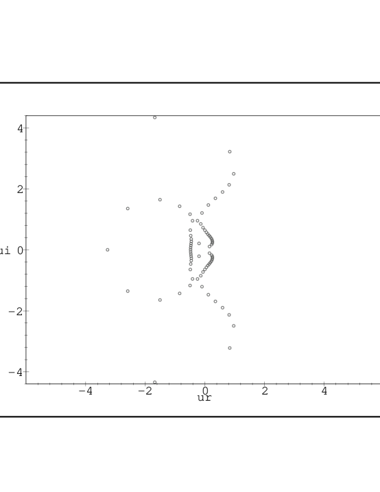
FIG. 19.: Zeros of $Z(L_{m},q,a)$ in the $u=1/a$ plane for $q=2.5$ and $m=24$ (i.e., $n=48$).

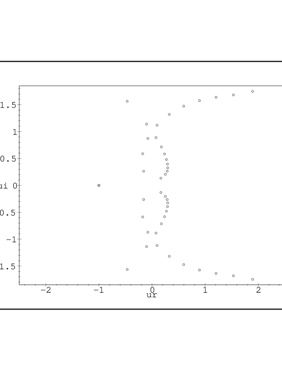
FIG. 20.: Same as Fig. 19 for $q=2$.

M ${\cal B}_{u}$ for $q=2$

Here we again encounter noncommutativity in the definition of the free energy and the locus ${\cal B}_{u}$. We first discuss $f_{nq}$ and $({\cal B}_{u})_{nq}$, obtained by setting $q=2$ and then taking $n\to\infty$. For $q=2$, besides the $q$-independent $\lambda_{L,1}=(a-1)^{2}$, we have

$$\lambda_{L,2}=(a-1)(a+1)$$ (152)

$$\lambda_{L,3}=a(a-1)(a+1)$$ (153)

$$\lambda_{L,4}=(a-1)^{2}$$ (154)

$$\lambda_{L,(5,6)}=\frac{1}{2}(a+1)\biggl{[}a^{2}+1\pm\Bigl{(}a^{4}-4a^{3}+10a^{2}-4a+1\Bigr{)}^{1/2}\ \biggr{]}$$ (155)

so that for this value of $q$, $\lambda_{L,1}=\lambda_{L,4}$. Further, $c_{L,1}=-c_{L,4}=-1$ so that the $(\lambda_{L,1})^{m}$ and $(\lambda_{L,4})^{m}$ terms cancel each other in $Z$, which reduces to

$$Z(L_{m},q=2,a)=\sum_{j=2,3,5,6}(\lambda_{L,j})^{m}\ .$$ (156)

Since each of the $\lambda_{j}$’s contributing to $Z(L_{m},q=2,a)$ has an $(a+1)$ factor, it follows that

$$Z(L_{m},q=2,a)=2(a+1)^{m}\times polyn.$$ (157)

The result (157) implies that $Z(L,q=2,a=-1,m)=0$, which is implied more generally by our earlier Theorem 6 of Ref. [55]. This theorem states that for lattices with odd coordination number, the (zero-field) partition function of the Ising model vanishes at $a=-1$. This point may or may not be on $({\cal B}_{u})_{nq}$; for example, for the honeycomb lattice, it is, while for the Archimedean 3-12 lattice it is not [55]. In the present case we will find that it is not on $({\cal B}_{u})_{nq}$.

In Fig. 20 we show a plot of Fisher zeros for the $q=2$ case. Because of the general fact that $({\cal B}_{u})_{nq}$ passes through $u=0$ and the special inversion symmetry (15), (27) that holds for $q=2$, it follows that $({\cal B}_{u})_{nq}$ passes through $a=0$ also. The complex-temperature phase diagram consists of six phases, bounded by the locus ${\cal B}_{u}$ which is the continuous accumulation set of the Fisher zeros. The phase diagram in the $u$ plane consists of (i) the complex-temperature extension of the ${\mathbb{Z}}_{2}$-symmetric, paramagnetic phase, PM, including the real axis $u>0$, together with five O phases: (ii) $O_{1}$, including the interval on the imaginary $u$ axis from $u=0$ to $u=i$, and its complex-conjugate, (iii) $O_{1}^{*}$; (iv) $O_{2}$, including the interval on the imaginary axis from $u=i$ to $u=i\infty$, and (v) its complex conjugate, $O_{2}^{*}$; and (vi) $O_{3}$, including the negative real axis, $u\leq 0$. The PM and $O_{3}$ phases map to themselves under the inversion $u\to 1/u=a$, while $O_{1}\leftrightarrow O_{2}^{*}$ and $O_{2}\leftrightarrow O_{1}^{*}$ under this inversion. As in our previous work [54, 55] we shall henceforth suppress the qualifier (CTE) and refer to the PM phase simply as the PM phase. In this phase, $\lambda_{L,5}$ is the dominant term in (95) so that reduced free energy is given by $f=(1/2)\ln\lambda_{L,5}$ in the PM phase, as in (142). In other regions that are not analytically connected with the PM region, only $|e^{f}|$ can be determined unambiguously:

$$|e^{f}|=|\lambda_{L,5}|^{1/2}\quad{\rm for}\quad u\in O_{3},O_{3}^{*}$$ (158)

$$|e^{f}|=|\lambda_{L,3}|^{1/2}\quad{\rm for}\quad u\in O_{1},O_{1}^{*}$$ (159)

and

$$|e^{f}|=|\lambda_{L,2}|^{1/2}\quad{\rm for}\quad u\in O_{2},O_{2}^{*}\ .$$ (160)

where here $f=f_{nq}$. The locus ${\cal B}_{u}$ has multiple points (in the algebraic geometry sense) at $u=0$ and $u=\pm i$ and at complex infinity, i.e., at $a=1/u=0$ corresponding to the zero-temperature ferromagnetic and antiferromagnetic Ising critical points. We have also calculated $Z(G,q,v)$ exactly for the Ising model on the cyclic $L_{y}=3$ strip and have found that ${\cal B}_{u}$ again has multiple points at $u=\pm i$ (as well as at $u=0$ and $1/u=0$). A possible inference would be that this is true for cyclic or Möbius strips of the square graph for all finite values of $L_{y}\geq 2$. Given our exact results for $L_{y}=2,3$, we see once again a very interesting connection with the complex-temperature phase diagram of the same model – in this case, the Ising model – on the two-dimensional square lattice, for which ${\cal B}_{a}$ consists of the Fisher circles $|u\pm 1|=\sqrt{2}$, which intersect precisely in the points $u=\pm i$.

If one takes $n\to\infty$ first and then $q\to 2$, the resulting locus $({\cal B}_{u})_{qn}$ differs from $({\cal B}_{u})_{nq}$ in several respects. First, $({\cal B}_{u})_{qn}$ does not satisfy the inversion symmetry (27). Second, while $\lambda_{L,5,u}$ is dominant on the negative $u$ axis in the vicinity of the origin $u=0$, $\lambda_{L,1,u}$ (equal, in the $q\to 2$ limit, to $\lambda_{L,4,u}$) becomes dominant for $u<-0.454$ and similarly for radial paths emanating outward from the origin in the upper and lower $Re(u)<0$ half-plane. This gives rise to another region boundary. (Recall that the contributions of these $\lambda$’s cancelled if one took $q=2$ first, so that they did not affect $Z$ or the locus $({\cal B})_{nq}$ in the $n\to\infty$ limit.) The absence of the inversion symmetry in $({\cal B}_{u})_{qn}$ is clear since a region boundary on this locus passes through $u\simeq-0.454$ but not the inverse of this point. This is, then, an example of the noncommutativity $({\cal B}_{u})_{qn}\neq({\cal B}_{u})_{nq}$ for a case where both of these loci are nontrivial. Finally, one can also discuss ${\cal B}_{u}$ for negative real $q$ and for complex $q$, but we shall forgo this.

VII Summary and Conclusions

In summary, we have calculated exact closed-form expressions for the Potts model/random cluster partition function for general $q$ and temperature $T$, or equivalently, the Whitney/Tutte polynomial for the open, cyclic, and Möbius square strips (ladder graphs) of width $L_{y}=2$ and arbitrary length $L_{x}$. Taking the limit $L_{x}\to\infty$, we have determined the free energy $f$ (and $|e^{f}|$ in unphysical phases) and the continuous locus ${\cal B}$ where the free energy is singular, which arises as the continuous accumulation set of the partition function zeros in the ${\mathbb{C}}^{2}$ space of the variables $q$ and $u$. The divergences in the correlation length and susceptibility of the Potts ferromagnet at its zero-temperature critical point were shown to be more rapidly approached as the strip width increases, and the physical reason for this was given. Our comparison of different strip widths suggests the inference that for infinite-length, width $L_{y}$ cyclic (or Möbius) strip graphs, as $L_{y}\to\infty$, an infinite number of curves on ${\cal B}_{u}$ pass through the point $u=0$ and the Fisher zeros become dense in the neighborhood of this point. It was shown that the Potts/random cluster antiferromagnet on both the infinite-length circuit graph and ladder graph with cyclic or Möbius boundary conditions exhibits a phase transition at finite temperature if $0<q<2$, but with unphysical properties. We discussed a subtlety in the definition of the free energy of the random cluster model due to the noncommutativity at certain special values $q_{s}$: $\lim_{n\to\infty}\lim_{q\to q_{s}}Z^{1/n}\neq\lim_{q\to q_{s}}\lim_{n\to\infty}Z^{1/n}$. Several generalizations of results for the $T=0$ limit of the Potts antiferromagnet (chromatic polynomials) were presented. Among these is the general form (29) for the partition function of recursive strip graphs (and its further generalization to the case of nonzero external field, (35)). The analysis of [25] for the singular locus ${\cal B}_{q}$ in the case of chromatic polynomials was generalized to the present case of the full temperature-dependent Potts partition function. The dependence of the locus ${\cal B}$ as a function of the longitudinal boundary conditions was studied, and it was shown that this locus is the same for the strips considered here with cyclic and twisted cyclic (Möbius) longitudinal boundary conditions. For the Potts antiferromagnet, it was found that as the temperature increases from 0 to infinity, the singular locus ${\cal B}_{q}$ contracts in to the origin, $q=0$. For the Potts ferromagnet, this locus was found not to cross the positive $q$ axis, in contrast to the antiferromagnetic case, where, for the cyclic strip, it does. In both the antiferromagnet and ferromagnet cases, for the strips studied here, ${\cal B}_{q}$ passes (does not pass) through $q=0$ if one uses periodic (free) longitudinal boundary conditions. Generalizing our previous result for chromatic polynomials, we found that for the strips with periodic longitudinal boundary conditions, ${\cal B}_{q}$ encloses regions in the $q$ plane for values of $a$ where it is nontrivial (i.e., $a\neq 1$). Several advantages of periodic, as opposed to free, longitudinal boundary conditions were noted, including the fact that with such periodic longitudinal boundary conditions, the locus ${\cal B}_{u}$ passes through $u=0$, in 1-1 correspondence with the zero-temperature critical point of the Potts ferromagnet. Finally, certain properties of the complex-temperature phase diagrams and loci ${\cal B}_{u}$ for these infinite-length, finite-width strips were shown to be the same as known properties of the model on the square lattice, including the multiple points at $u=\pm i$ for $q=2$, which also occur in the exactly solved square-lattice Ising model and the point $u=-1/2$ for $q=3$, which is known to lie on ${\cal B}_{u}$ for the square lattice since it is dual to the zero-temperature critical point at $a=0$. This shows that exact solutions on infinite-length strips could provide a way of generating plausible conjectures for complex-temperature properties of the Potts model on two-dimensional lattices and some conjectures were made.

I would like to thank Prof. N. L. Biggs for kindly sending me a copy of [23] and Prof. F. Y. Wu for discussions, particularly on spanning trees, and for hospitality during a visit to the National Center for Theoretical Science (NCTS) and Academia Sinica, Taiwan, when some of this research was performed. I have also benefited from recent collaborations with H. Kluepfel and S.-C. Chang [45, 46] and thank A. Sokal and J. Salas for informing me about their work. The present research was supported in part at Stony Brook by the NSF grant PHY-97-22101 and at Brookhaven by the U.S. DOE contract DE-AC02-98CH10886.

VIII Appendix

A Connection Between Potts Model Partition Function and Tutte Polynomial

The Potts model partition function $Z(G,q,v)$ is related to the Tutte polynomial $T(G,x,y)$ as follows. The graph $G$ has vertex set $V$ and edge set $E$, denoted $G=(V,E)$. A spanning subgraph $G^{\prime}$ is defined as a subgraph that has the same vertex set and a subset of the edge set: $G^{\prime}=(V,E^{\prime})$ with $E^{\prime}\subseteq E$. The Tutte polynomial of $G$, $T(G,x,y)$, is then given by [7]-[9]

$$T(G,x,y)=\sum_{G^{\prime}\subseteq G}(x-1)^{k(G^{\prime})-k(G)}(y-1)^{c(G^{\prime})}$$ (161)

where $k(G^{\prime})$, $e(G^{\prime})$, and $n(G^{\prime})=n(G)$ denote the number of components, edges, and vertices of $G^{\prime}$, and

$$c(G^{\prime})=e(G^{\prime})+k(G^{\prime})-n(G^{\prime})$$ (162)

is the number of independent circuits in $G^{\prime}$ (sometimes called the co-rank of $G^{\prime}$). Note that the first factor can also be written as $(x-1)^{r(G)-r(G^{\prime})}$, where

$$r(G)=n(G)-k(G)$$ (163)

is called the rank of $G$. The graphs $G$ that we consider here are connected, so that $k(G)=1$. Now let

$$x=1+\frac{q}{v}$$ (164)

and

$$y=a=v+1$$ (165)

so that $q=(x-1)(y-1)=(x-1)v$. Then

$$Z(G,q,v)=(x-1)^{k(G)}(y-1)^{n(G)}T(G,x,y)\ .$$ (166)

There is also a connection with the Whitney rank polynomial, $R(G,\xi,\eta)$, defined as [4, 12]

$$R(G,\xi,\eta)=\sum_{G^{\prime}\subseteq G}\xi^{r(G^{\prime})}\eta^{c(G^{\prime})}$$ (167)

where the sum is again over spanning subgraphs $G^{\prime}$ of $G$. Then

$$T(G,x,y)=(x-1)^{r(G)}R(G,\xi=(x-1)^{-1},\eta=y-1)$$ (168)

and

$$Z(G,q,v)=q^{n(G)}R(G,\xi=\frac{v}{q},\eta=v)\ .$$ (169)

Note that the chromatic polynomial is a special case of the Tutte polynomial:

$$P(G,q)=q^{k(G)}(-1)^{k(G)+n(G)}T(G,x=1-q,y=0)$$ (170)

(recall eq. (10)).

From the representation (166) and the duality property of the Tutte polynomial

$$T(G,x,y)=T(G^{*},y,x)$$ (171)

where $G^{*}$ is the dual graph corresponding to $G$, it follows that

$$Z(G,q,v)=v^{e(G)}q^{-c(G)}Z(G^{*},q,v_{d})$$ (172)

where $G^{*}$ denotes the graph that is dual to $G$ and $v_{d}$ is the dual image of $v$:

$$v_{d}=\frac{q}{v}$$ (173)

or equivalently, in terms of the variable $a$,

$$a_{d}=\frac{a-1+q}{a-1}\ .$$ (174)

Corresponding to the form (29) we find that the Tutte polynomial for recursively defined graphs comprised of $m$ repetitions of some subgraph has the form

$$T(G_{m},x,y)=\sum_{j=1}^{N_{\lambda}}c_{T,G,j}(\lambda_{T,G,j})^{m}$$ (175)

B Square Strip with Free Longitudinal Boundary Conditions

The generating function representation for the Tutte polynomial for the open square strip $S_{m}$ is

$$\Gamma_{T}(S_{m},x,y;z)=\sum_{m=0}^{\infty}T(S_{m},x,y)z^{m}\ .$$ (176)

We have

$$\Gamma_{T}(S,x,y;z)=\frac{{\cal N}_{T}(S,x,y;z)}{{\cal D}_{T}(S,x,y;z)}$$ (177)

where

$${\cal N}_{T}(S,x,y;z)=A_{T,S,0}+A_{T,S,1}z=(y+x+x^{2}+x^{3})-yx^{3}z$$ (178)

and

$${\cal D}_{T}(S,x,y,z) = 1-(y+1+x+x^{2})z+yx^{2}z^{2}$$ (179)

$$= \prod_{j=1}^{2}(1-\lambda_{T,S,j}z)$$ (181)

with

$$\lambda_{T,S,(1,2)}=\frac{1}{2}\biggl{[}(1+y+x+x^{2})\pm\Bigl{(}y^{2}+2y(1+x-x^{2})+(x^{2}+x+1)^{2}\Bigr{)}^{1/2}\biggr{]}\ .$$ (182)

The corresponding closed-form expression is given by the general formula from [34], as applied to Tutte, rather than chromatic, polynomials, namely

$$T(S_{m},x,y)=\biggl{[}\frac{A_{T,S,0}\lambda_{T,S,1}+A_{T,S,1}}{\lambda_{T,S,1}-\lambda_{T,S,2}}\biggr{]}(\lambda_{T,S,1})^{m}+\biggl{[}\frac{A_{T,S,0}\lambda_{T,S,2}+A_{T,S,1}}{\lambda_{T,S,2}-\lambda_{T,S,1}}\biggr{]}(\lambda_{T,S,2})^{m}\ .$$ (183)

An alternative expression for $T$ that explicitly shows that it is a symmetric function of the $\lambda_{S,j}$, $j=1,2$, is

$$T(S_{m},x,y)=\frac{1}{2}(y+x+x^{2}+x^{3})\Bigl{[}(\lambda_{T,S,1})^{m}+(\lambda_{T,S,2})^{m}\Bigr{]}+$$ (184)

(185)

$$\frac{1}{2}\Bigl{[}y^{2}+y+2yx+2yx^{2}+x+2x^{2}+3x^{3}+2x^{4}-yx^{3}+x^{5}\Bigr{]}\Biggl{[}\frac{(\lambda_{T,S,1})^{m}-(\lambda_{T,S,2})^{m}}{\lambda_{T,S,1}-\lambda_{T,S,2}}\Biggr{]}\ .$$ (186)

C Cyclic and Möbius Square Strips

We write the Tutte polynomials for the cyclic and Möbius square strips $L_{m}$ and $ML_{m}$ as

$$T(L_{m},x,y)=\sum_{j=1}^{6}c_{T,L,j}(\lambda_{T,L,j})^{m}$$ (187)

and

$$T(ML_{m},x,y)=\sum_{j=1}^{6}c_{T,ML,j}(\lambda_{T,ML,j})^{m}$$ (188)

where it is convenient to extract a common factor from the coefficients:

$$c_{T,G,j}\equiv\frac{\bar{c}_{T,G,j}}{x-1}\ ,\quad G=L,ML\ .$$ (189)

Of course, although the individual terms contributing to the Tutte polynomial are thus rational functions of $x$ rather than polynomials in $x$, the full Tutte polynomial is a polynomial in both $x$ and $y$. We have

$$\lambda_{T,ML,j}=\lambda_{T,L,j}\ ,\quad j=1,...,6$$ (190)

$$\lambda_{T,L,1}=1$$ (191)

$$\lambda_{T,L,2}=x$$ (192)

$$\lambda_{T,L,(3,4)}=\frac{1}{2}\biggl{[}x+y+2\pm\Bigl{(}(x-y)^{2}+4(x+y+1)\Bigr{)}^{1/2}\ \biggr{]}$$ (193)

and

$$\lambda_{T,L,5}=\lambda_{T,S,1}\ ,\quad\lambda_{T,L,6}=\lambda_{T,S,2}\ .$$ (194)

Our result for $T(G,x,y)$, $G=L,ML$ agrees with a recursion relation given in [22] (see also [23]).

$$\bar{c}_{T,L,1}=[(x-1)(y-1)]^{2}-3(x-1)(y-1)+1$$ (195)

$$\bar{c}_{T,L,2}=\bar{c}_{T,L,3}=\bar{c}_{T,L,4}=xy-x-y$$ (196)

$$\bar{c}_{T,L,5}=\bar{c}_{T,L,6}=1$$ (197)

$$\bar{c}_{T,ML,1}=-1$$ (198)

$$\bar{c}_{T,ML,2}=-xy+x+y$$ (199)

$$\bar{c}_{T,ML,3}=\bar{c}_{ML,4}=xy-x-y$$ (200)

$$\bar{c}_{T,ML,5}=\bar{c}_{T,ML,6}=1\ .$$ (201)

We note that $\lambda_{T,L,3}\lambda_{T,L,4}=xy$ and $\lambda_{T,L,5}\lambda_{T,L,6}=x^{2}y$.

D Special Values of Tutte Polynomials for Square Strips

For a given graph $G=(V,E)$, at certain special values of the arguments $x$ and $y$, the Tutte polynomial $T(G,x,y)$ yields quantities of basic graph-theoretic interest [11]-[14], citewu77-[79]. We recall some definitions: a spanning subgraph $G^{\prime}=(V,E^{\prime})$ of $G$ is a graph with the same vertex set $V$ and a subset of the edge set, $E^{\prime}\subseteq E$. Furthermore, a tree is a graph with no cycles, and a forest is a graph containing one or more trees. Then the number of spanning trees of $G$, $N_{ST}(G)$, is

$$N_{ST}(G)=T(G,1,1)\ ,$$ (202)

the number of spanning forests of $G$, $N_{SF}(G)$, is

$$N_{SF}(G)=T(G,2,1)\ ,$$ (203)

the number of connected spanning subgraphs of $G$, $N_{CSSG}(G)$, is

$$N_{CSSG}(G)=T(G,1,2)\ ,$$ (204)

and the number of spanning subgraphs of $G$, $N_{SSG}(G)$, is

$$N_{SSG}(G)=T(G,2,2)\ .$$ (205)

Clearly, $N_{SSG}(G)-N_{CSSG}(G)$ is the number of disconnected spanning subgraphs of $G$ and $N_{CSSG}(G)-N_{ST}(G)$ is the number of connected spanning subgraphs of $G$ that contain one or more cycles. One thus has the inequality

$$N_{SSG}(G)\geq N_{CSSG}(G)\geq N_{ST}(G)\quad i.e.,\quad T(G,2,2)\geq T(G,1,2)\geq T(G,1,1)\ .$$ (206)

Also, clearly

$$N_{SSG}(G)\geq N_{SF}(G)\quad i.e.,\quad T(G,2,2)\geq T(G,2,1)$$ (207)

and

$$N_{SF}(G)\geq N_{ST}(G)\quad i.e.,\quad T(G,2,1)\geq T(G,1,1)\ .$$ (208)

The set of spanning forests differs from the set of connected spanning subgraphs by the removal of the condition that the subgraph is connected but the imposition of the condition that the subgraph have no cycles, and hence there is no general inequality between $N_{SF}(G)$ and $N_{CSSG}(G)$.

We recall the results for tree graphs $T_{n}$ and circuit graphs $C_{n}$: $T(T_{n},1,1)=T(T_{n},1,2)=1$, $T(T_{n},2,1)=T(T_{n},2,2)=2^{n-1}$, $T(C_{n},1,1)=n$, $T(C_{n},2,1)=2^{n}-1$, $T(C_{n},1,2)=n+1$, and $T(C_{n},2,2)=2^{n}$.

For the open square strip $S_{m}$ we find

$$N_{ST}(S_{m})=2\Bigl{[}(2+\sqrt{3}\ )^{m}+(2-\sqrt{3}\ )^{m}\Bigr{]}+\frac{7}{2\sqrt{3}}\Bigl{[}(2+\sqrt{3}\ )^{m}-(2-\sqrt{3}\ )^{m}\Bigr{]}$$ (209)

$$N_{SF}(S_{m})=\frac{15}{2}\biggl{[}(2(2+\sqrt{3}))^{m}+(2(2-\sqrt{3}))^{m}\biggr{]}+\frac{13}{\sqrt{3}}\biggl{[}(2(2+\sqrt{3}))^{m}-(2(2-\sqrt{3}))^{m}\biggr{]}$$ (210)

$$N_{CSSG}(S_{m})=\frac{5}{2}\biggl{[}\biggl{(}\frac{5+\sqrt{17}}{2}\ \biggr{)}^{m}+\biggl{(}\frac{5-\sqrt{17}}{2}\ \biggr{)}^{m}\biggr{]}+\frac{21}{2\sqrt{17}}\biggl{[}\biggl{(}\frac{5+\sqrt{17}}{2}\ \biggr{)}^{m}-\biggl{(}\frac{5-\sqrt{17}}{2}\ \biggr{)}^{m}\biggr{]}$$ (211)

and

$$N_{SSG}(S_{m})=2^{3m+4}\ .$$ (212)

That eqs. (209)-(211) yield integers follows from the theorem on symmetric polynomial functions of roots of an algebraic equation, as discussed in [41].

With the definition

$$\eta_{G}=\cases{+1&if $G=L$\cr-1&if $G=ML$\cr}$$ (213)

our calculations of the Tutte polynomials for the cyclic strip $L_{m}$ and the Möbius strip $ML_{m}$ yield

$$N_{ST}(G_{m})=m\biggl{\{}-\eta_{G}+\frac{1}{2}\biggl{[}(2+\sqrt{3})^{m}+(2-\sqrt{3})^{m}\biggr{]}\biggr{\}}\ ,\quad G_{m}=L_{m},\ ML_{m}$$ (214)

$$N_{SF}(G_{m}) = \eta_{G}(1-2^{m})-\biggl{[}\biggl{(}\frac{5+\sqrt{17}}{2}\ \biggr{)}^{m}+\biggl{(}\frac{5-\sqrt{17}}{2}\ \biggr{)}^{m}\biggr{]}$$ (215)

$$+ \Bigl{(}2(2+\sqrt{3})\Bigr{)}^{m}+\Bigl{(}2(2-\sqrt{3})\Bigr{)}^{m}\ ,\quad G_{m}=L_{m},\ ML_{m}$$ (217)

$$N_{CSSG}(L_{m}) = N_{CSSG}(ML_{m})-2m-1=-(m+2)+\frac{(m+2)}{2}\biggl{[}\biggl{(}\frac{5+\sqrt{17}}{2}\ \biggr{)}^{m}+\biggl{(}\frac{5-\sqrt{17}}{2}\ \biggr{)}^{m}\biggr{]}$$ (220)

$$-\frac{m}{2\sqrt{17}}\biggl{[}\biggl{(}\frac{5+\sqrt{17}}{2}\ \biggr{)}^{m}-\biggl{(}\frac{5-\sqrt{17}}{2}\ \biggr{)}^{m}\biggr{]}$$

and

$$N_{SSG}(L_{m})=N_{SSG}(ML_{m})=2^{3m}\ .$$ (221)

The results for the spanning trees for the cyclic and Möbius strips are known [76] (for higher-dimensions, see [79]); we are not aware of the other quantities having been published.

Several comments are in order. Since $T(G_{m},x,y)$ grows exponentially as $m\to\infty$ for the families $G_{m}=S_{m}$, $L_{m}$, and $ML_{m}$ for $(x,y)=(1,1)$, (2,1), (1,2), and (2,2) (as well as for $G_{m}=C_{m}$ and $T_{m}$ for $(x,y)=(2,1)$ and (2,2)), it is natural to define corresponding constants

$$z_{set}(\{G\})=\lim_{n(g)\to\infty}n(G)^{-1}\ln N_{x}(G)\ ,\quad set=ST,\ SF,\ CSSG,\ SSG$$ (222)

where, as above, the symbol $\{G\}$ denotes the limit of the graph family $G$ as $n(G)\to\infty$ (and the $z$ here should not be confused with the auxiliary expansion variable in the generating function (176) or the Potts partition function $Z(G,q,v)$.) The general inequalities (206), (207), and (208) imply that, for a given $\{G\}$,

$$z_{SSG}\geq z_{CSSG}\geq z_{ST}$$ (223)

$$z_{SSG}\geq z_{SF}$$ (224)

and

$$z_{SF}\geq z_{ST}\ .$$ (225)

We find that for both the line $(L_{y}=1$) and the $L_{y}=2$ square strip, the quantity $z_{set}(\{G\})$ is independent of whether the longitudinal boundary conditions are free, periodic, or Möbius:

$$z_{ST}(\{G\})=\frac{1}{2}\ln(2+\sqrt{3})\simeq 0.658479\quad{\rm for}\quad G=S,L,ML$$ (226)

$$z_{SF}(\{G\})=\frac{1}{2}\ln[2(2+\sqrt{3}\ )]\simeq 1.00505\quad{\rm for}\quad G=S,L,ML$$ (227)

$$z_{CSSG}(\{G\})=\frac{1}{2}\ln\Biggl{(}\frac{5+\sqrt{17}}{2}\Biggr{)}\simeq 0.758832\quad{\rm for}\quad G=S,L,ML$$ (228)

and

$$z_{SSG}(\{G\})=\frac{3}{2}\ln 2\simeq 1.03972\quad{\rm for}\quad G=S,L,ML$$ (229)

(where the result for $z_{ST}$ can be extracted from [76]).

E Tutte Polynomials for Dual Graphs

Since the Tutte polynomial satisfies the duality relation (171), our calculations of the Tutte polynomials $T(G_{m},x,y)$ for the open, cyclic, and Möbius square strips, $G_{m}=S_{m}$, $L_{m}$, and $ML_{m}$, also yield the corresponding results for the duals of these graphs. The dual of the square $L_{y}=2$ strip with $m+1$ squares, i.e., length $L_{x}=m+1$ edges, $(S_{m})^{*}$, can be described as follows: for $m\geq 1$, consider a line of $m+1$ vertices, with successive vertices $v_{i}$ and $v_{i+1}$ connected to each other by an edge $e_{i}$; the vertices on this line are connected to a single external vertex by double edges, except for the first and last vertices on the line, each of which is connected to the external vertex via three edges. This is $(S_{m})^{*}$ for $m\geq 1$. Note that this is a multigraph, since a (proper) graph is normally defined not to have loops or multiple edges. For the case $m=0$, i.e., a single square, the dual is $(S_{1})^{*}=TL_{4}$, where in the mathematical literature, $TL_{\ell}$, denoted “thick link”, is the multigraph consisting of two vertices connected by $\ell$ edges. Our results for $T(S_{m},x,y)$ in eq. (183) thus give the Tutte polynomial for this dual graph as $T((S_{m})^{*},x,y)=T(S_{m},y,x)$.

For the dual of the cyclic strip graph, $(L_{m})^{*}$, we recall a definition from graph theory: given two graphs $G$ and $H$, the “join” $G+H$ is the graph obtained by connected each vertex of $G$ to each vertex of $H$ with edges. We also recall the notation $\bar{K}_{p}$ for the complement of $K_{p}$, i.e. the graph consisting of $p$ vertices with no edges. Then for $m\geq 3$,

$$(L_{m})^{*}=\bar{K}_{2}\ +\ C_{m}$$ (230)

where $C_{m}$ is the circuit graph with $m$ vertices. Hence our results for $T(L_{m},x,y)$ in eqs. (95) with (98)-(104) also determine $T((L_{m})^{*},x,y)=T(L_{m},y,x)$.

REFERENCES

- [1] R. B. Potts, Proc. Camb. Phil. Soc. 48 106 (1952).
- [2] F. Y. Wu, Rev. Mod. Phys. 54 (1982) 235.
- [3] G. D. Birkhoff, Ann. of Math. 14 (1912) 42.
- [4] H. Whitney, Ann. of Math. 33 (1932) 688.
- [5] G. D. Birkhoff and D. Lewis, Trans. Amer. Math. Soc. 60 (1946) 355.
- [6] P. W. Kasteleyn and C. M. Fortuin, J. Phys. Soc. Jpn. 26 (1969) (Suppl.) 11; C. M. Fortuin and P. W. Kasteleyn, Physica 57 (1972) 536.
- [7] W. T. Tutte, Proc. Cam. Phil. Soc. 43 (1947) 26.
- [8] W. T. Tutte, Can. J. Math. 6 (1954) 80.
- [9] W. T. Tutte, J. Combin. Theory 2 (1967) 301.
- [10] W. T. Tutte, “Chromials”, in Lecture Notes in Math. v. 411 (1974) 243.
- [11] W. T. Tutte, Graph Theory, vol. 21 of Encyclopedia of Mathematics and Applications (Addison-Wesley, Menlo Park, 1984).
- [12] N. L. Biggs, Algebraic Graph Theory (2nd ed., Cambridge Univ. Press, Cambridge, 1993).
- [13] D. J. A. Welsh, Complexity: Knots, Colourings, and Counting, London Math. Soc. Lect. Note Ser. 186 (Cambridge University Press, Cambridge, 1993).
- [14] B. Bollobás, Modern Graph Theory (Springer, New York, 1998).
- [15] L. Onsager, Phys. Rev. 65 (1944) 117.
- [16] See, e.g., J. Cardy, in C. Domb and J. L. Lebowitz, eds., Phase Transitions and Critical Phenomena (Academic Press, New York, 1987), vol. 11, p. 55; C. Itzykson, H. Saleur, and J.-B. Zuber, Conformal Invariance and Applications to Statistical Mechanics (World Scientific, Singapore, 1988); P. Di Francesco, P. Mathieu, and D. Sénéchal, Conformal Field Theory (Springer, New York, 1997), and references therein.
- [17] E. H. Lieb, Phys. Rev. 162, 162 (1967).
- [18] M. Aizenman and E. H. Lieb, J. Stat. Phys. 24 (1981) 279; Y. Chow and F. Y. Wu, Phys. Rev. B36 (1987) 285.
- [19] R. C. Read, J. Combin. Theory 4 (1968) 52.
- [20] R. C. Read and W. T. Tutte, “Chromatic Polynomials”, in Selected Topics in Graph Theory, 3, eds. L. W. Beineke and R. J. Wilson (Academic Press, New York, 1988.).
- [21] R. Shrock and S.-H. Tsai, Phys. Rev. E55 (1997) 5165.
- [22] N. L. Biggs, R. M. Damerell, and D. A. Sands, J. Combin. Theory B 12 (1972) 123.
- [23] Sands, D. A., Ph.D. Thesis, Univ. of London, 1972 (unpublished).
- [24] N. L. Biggs and G. H. Meredith, J. Combin. Theory B20 (1976) 5; N. L. Biggs, Bull. London Math. Soc. 9 (1976) 54.
- [25] S. Beraha, J. Kahane, and N. Weiss, J. Combin. Theory B 27 (1979) 1; ibid. 28 (1980) 52.
- [26] R. C. Read, in Proc. 3rd Caribbean Conf. on Combin. and Computing (1981); Proc. 5th Caribbean Conf. on Combin. and Computing (1988).
- [27] R. J. Baxter, J. Phys. A 20 (1987) 5241.
- [28] R. C. Read and G. F. Royle, in Graph Theory, Combinatorics, and Applications (Wiley, NY, 1991), vol. 2, p. 1009.
- [29] R. C. Read and E. G. Whitehead, Discrete Math. 204 (1999) 337 and unpublished reports.
- [30] R. Shrock and S.-H. Tsai, Phys. Rev. E56 (1997) 1342, 2733, 3935, 4111.
- [31] R. Shrock and S.-H. Tsai, Phys. Rev. E58 (1998) 4332; cond-mat/9808057.
- [32] M. Roček, R. Shrock, and S.-H. Tsai, Physica A252 (1998) 505.
- [33] M. Roček, R. Shrock, and S.-H. Tsai, Physica A259 (1998) 367.
- [34] R. Shrock and S.-H. Tsai, Physica A259 (1998) 315.
- [35] R. Shrock and S.-H. Tsai, J. Phys. A 31 (1998) 9641; Physica A265 (1999) 186.
- [36] R. Shrock and S.-H. Tsai, J. Phys. A Lett. 32 (1999) L195.
- [37] R. Shrock and S.-H. Tsai, Phys. Rev. E60 (1999) 3512; Physica A 275 (1999) 429.
- [38] A. Sokal, Combin. Prob. Comput., in press (cond-mat/9904146); cond-mat/9910503.
- [39] R. Shrock and S.-H. Tsai, J. Phys. 32 (1999) 5053.
- [40] N. L. Biggs, LSE report LSE-CDAM-99-03 (May 1999), to appear.
- [41] R. Shrock, Phys. Lett. A261 (1999) 57.
- [42] N. L. Biggs and R. Shrock, J. Phys. A (Letts) 32, L489 (1999).
- [43] R. Shrock, in the Proceedings of the 1999 British Combinatorial Conference, BCC99 (July, 1999), Discrete Math., to appear.
- [44] R. Shrock, in the Proceedings of the Taiwan Conference on Equilibrium and Non-Equilibrium Phase Transitions (Academia Sinica, Taipei, Aug. 1999).
- [45] H. Kluepfel and R. Shrock, YITP-99-32,33; H. Kluepfel, Stony Brook thesis (July, 1999).
- [46] S.-C. Chang and R. Shrock, YITP-SB-99-50,58.
- [47] J. Salas and A. Sokal, work in progress.
- [48] e.g. G. Berman and W. T. Tutte, J. Combin. Theory 6 (1969) 301; D. Woodall, Discrete Math. 101 (1992) 333; B. Jackson, Combin. Prob. Comput. 2 (1993) 325; F. Brenti, G. Royle, and D. Wagner, Canad. J. Math. 46 (1994) 55; V. Thomassen, Combin. Prob. Comput. 6 (1997) 497; J. Brown, J. Brown, J. Combin. Theory 6 B (1998) 251.
- [49] C. Itzykson, R. B. Pearson, and J.-B. Zuber, Nucl. Phys. B220 (1983) 415.
- [50] V. Matveev and R. Shrock, J. Phys. A 28 (1995) 4859; Phys. Rev. E53 (1996) 254; Phys. Lett. A215 (1996) 271.
- [51] T. D. Lee and C. N. Yang, Phys. Rev. 87 (1952) 410; C. N. Yang and T. D. Lee, ibid, 87 (1952) 404.
- [52] M. E. Fisher, Lectures in Theoretical Physics (Univ. of Colorado Press, Boulder, 1965), vol. 7C, p. 1.
- [53] S.-Y. Kim, R. Creswick, C.-N. Chen, and C.-K. Hu, in the Proceedings of the Taiwan Conference on Equilibrium and Non-Equilibrium Phase Transitions (Academia Sinica, Taipei, Aug. 1999).
- [54] V. Matveev and R. Shrock, J. Phys. A 28 (1995) 1557.
- [55] V. Matveev and R. Shrock, J. Phys. A 28 (1995) 5235.
- [56] J. Salas and A. Sokal, J. Stat. Phys. 86 (1997) 551.
- [57] Y. K. Wang and F. Y. Wu, J. Phys. A 9 (1976) 593.
- [58] V. Matveev and R. Shrock, Phys. Lett. A204 (1995) 353.
- [59] P. P. Martin, J. Phys. A 19, 3267 (1986). See also P. P. Martin, ibid., 20, L601 (1986).
- [60] D. W. Wood, J. Phys. A 20, 3471 (1987); D. W. Wood, R. W. Turnbull, and J. K. Ball, ibid. 3495 (1987).
- [61] J. V. Uspensky, Theory of Equations (McGraw-Hill, NY 1948), 264.
- [62] R. Hartshorne, Algebraic Geometry (Springer, New York, 1977).
- [63] A. E. Ferdinand and M. E. Fisher, Phys. Rev. 185 (1969) 832.
- [64] M. E. Fisher and M. N. Barber, Phys. Rev. Lett. 28 (1972) 1516; M. N. Barber, in C. Domb and J. Lebowitz, Phase Transitions and Critical Phenomena, v. 8 (Wiley, New York, 1983).
- [65] V. Matveev and R. Shrock, J. Phys. A (Letts.) 28 (1995) L533.
- [66] J. M. Maillard and R. Rammal, J. Phys. A 16 (1983) 353.
- [67] P. P. Martin and J. M. Maillard, J. Phys. A 19 (1986) L547.
- [68] P. P. Martin, Potts Models and Related Problems in Statistical Mechanics (World Scientific, Singapore, 1991).
- [69] C. N. Chen, C. K. Hu, and F. Y. Wu, Phys. Rev. Lett. 76 (1996) 169.
- [70] F. Y. Wu, G. Rollet, H. Y. Huang, J. M. Maillard, C. K. Hu, and C. N. Chen, Phys. Rev. Lett. 76 (1996) 173.
- [71] V. Matveev and R. Shrock, Phys. Rev. E54 (1996) 6174.
- [72] R. Shrock and S.-H. Tsai, J. Phys. A 30 (1997) 495.
- [73] H. Feldmann, R. Shrock, and S.-H. Tsai, J. Phys. A (Lett.) 30 (1997) L663; Phys. Rev. E57 (1998) 1335; H. Feldmann, A. J. Guttmann, I. Jensen, R. Shrock, and S.-H. Tsai), J. Phys. A 31 (1998) 2287.
- [74] W.-Y. Kim and R. Creswick, Phys. Rev. E58 (1998) 7006.
- [75] R. J. Baxter, Proc. Roy. Soc. London, Ser. A 383 (1982) 43.
- [76] R. K. Guy and F. Harary, Univ. of Calgary Rept. 2, 1966; J. Sedlácek, in Combinatorial Structures and Applications (Gordon and Breach, New York, 1970), p. 387.
- [77] F. Y. Wu, J. Phys. A 10 (1977) L113.
- [78] F. Y. Wu, C. King, and W. T. Lu, Ann. Inst. Fourier 49 (1999) 101.
- [79] W.-J. Tzeng and F. Y. Wu, Northeastern-NCTS preprint; R. Shrock, F. Y. Wu, Northeastern-NCTS-Stony Brook preprint.