A planar extrapolation of the correlation problem that permits pairing

Abstract

It was observed previously that the $SU(N)$ extension of the Hubbard model is dominated by planar diagrams at large $N$, but the possibility of superconducting pairing got lost in this extrapolation. To allow for pairing, we replace $SU(N)$ by $U(N,q)$, the unitary group in a vector space of quaternions. At the level of the free energy, the difference between the $SU(N)$ and $U(N,q)$ extrapolations appears only to first nonleading order in $N$.

PACS Numbers: 71.27.+a 71.10.-w 71.10.Fd

I Introduction and Motivation

The Hubbard model [1] belongs to a class of models describing strongly correlated electrons in systems such as, for example, high $T_{c}$ ceramics, transition metal oxides and organic conductors[2]. However, in spite of much progress made over the last $\sim 40$ years, it is still difficult to determine the low temperature properties of such model systems as a function of their chemical input parameters.

Recently it was noticed [4] that an $SU(N)$ deformation of such models is dominated, for $N\gg 1$, by planar diagrams in the sense of ’t Hooft [3] and the sum of the leading planar diagrams turned out to be very similar to the ”Fluctuation Exchange Approximation (FLEX)” pioneered by Bickers and Scalapino [5]. However, unlike the FLEX approximation, the new method permits a systematic construction of the generating functional in powers of $1/N$.

To exploit this new perspective on the correlation problem, we should study the evolution of the properties of a given model as one moves from $N=\infty$ to $N=2$. But precisely such a study is impossible in the $SU(N)$ extrapolation of the Hubbard model since for $N>2$ it contains no analog of the superconducting order parameter $<\psi_{\alpha}(x)\varepsilon_{\alpha\beta}\psi_{\beta}(y)>$. The very feature that constituted one of the motivations of studying Hubbard like models in the first place got lost in this extrapolation.

Some time ago it was recognized[6], that $U(N,q)$, the unitary group acting in a vector space of quaternions, provides an interesting way of implementing the large $N$ limit because it generalizes the antisymmetric tensor $\varepsilon_{\alpha\beta}$ in a natural way. Because of $U(1,q)=SU(2)$, an extrapolation via $U(N,q)$ with $N=1,2,..$ is just as good an extrapolation as $SU(N)$ with $N=2,3..$ Results of what probably amounted to an $U(N,q)$ extrapolation of the $tJ$ model were given recently [7], but without any calculational details.

We will show below that there is a unique $U(N,q)$ extrapolation of the Hubbard model that permits pairing and, simultaneously, a topological expansion in which the planar diagrams dominate for $N\gg 1$.

II $U(N,q)$ invariant interactions between bosons and fermions

It is reasonable to begin our discussion by recalling the definition of the group $U(N,q)$ [8]. It acts in a vector space of quaternions:

$$\psi_{a} = \psi_{a,0}+i\sum_{r=1..3}\psi_{a,r}\sigma^{r}\text{ \ \ \ \ and\ \ \ \ \ \ }\psi_{a}^{\ast}=\psi_{a,0}-i\sum_{r=1..3}\psi_{a,r}\sigma^{r}$$ (2)

$$\psi_{a\mu}\text{ real for }a=1..N\text{, }\mu=0..3\text{, \ \ \ }\overrightarrow{\sigma}=\text{Pauli matrices}$$

The $\psi_{a\mu}$ are real because we wish to think of the matrices $i\sigma^{r}$, $r=1..3$ as square roots of $-1$. The transformation matrix $g$ is also quaternion valued, $g=g^{0}+i\overrightarrow{g}\overrightarrow{\sigma}$ with $g_{\mu}$, $\mu=0..3$ real in order for the image to be a quaternion. As a further constraint, it must leave a quaternion valued length invariant:

$$\sum_{a=1..N}\psi_{a}^{\ast}\psi_{a}=\sum_{a=1..N}(\psi^{\ast}g^{+})_{a}(g\psi)_{a}\rightarrow g^{+}g=1$$ (3)

The properties of the Pauli matrices $\overrightarrow{\sigma}$ imply $g^{T}=\sigma^{2}\left(g^{0}-i\overrightarrow{g}\overrightarrow{\sigma}\right)\sigma^{2}$ and $g^{+}=g^{0}-i\overrightarrow{g}\overrightarrow{\sigma}$ from which we deduce $g^{T}=\sigma^{2}g^{+}\sigma^{2}$. In conjunction with $g^{+}g=1$ this latter relation implies $g^{T}\sigma^{2}g=\sigma^{2}$. The relations

$$g^{+}g=1\text{ and }g^{T}\sigma^{2}g=\sigma^{2}$$ (4)

can be restated by saying that $U(N,q)$ has two invariant tensors,$\ \delta_{ab}\sigma_{\alpha\beta}^{2}$ and $\delta_{ab}\delta_{\alpha\beta}$.

The quaternions $\psi_{a}\rightarrow$ $\left(\psi_{a}\right)_{\sigma\tau}$ of eq(2) are not all independent because they can be parametrized by only 4 real quantities for each value of $a$. To get rid of the redundant quantities, while keeping the attractive transformation properties of the quaternions, we define ”conventional” complex electron operators

$$\psi_{a\sigma}=\sum_{\tau=1,2}\left(\psi_{a}\right)_{\sigma\tau}\xi_{\tau}\text{ \ \ , \ \ \ \ \ }\xi=\left(\begin{array}[]{c}1\\ 0\end{array}\right)$$ (5)

that have only one spinor index.

A nonvanishing average such as

$$<\sum\psi_{a\sigma}(x)\sigma_{\sigma\tau}^{2}\psi_{a\tau}(y)>\neq 0$$ (6)

breaks charge but conserves $U(N,q)$  and pairing is therefore possible in an $U(N,q)$ extension of the Hubbard model.

Following the strategy described in [4] we will introduce auxiliary boson fields via a Hubbard Stratonovich transformation. For this we need (i) an invariant quadratic form in the auxiliary bosons and (ii) an invariant interaction between the auxiliary bosons and some fermion bilinears. Both requirements are met if the auxiliary fields are infinitesimal generators of $U(N,q)$, so we consider them now. Writing finite transformations as $g=\exp iz$ ,   $z=iz_{0}+\overrightarrow{z}\overrightarrow{\sigma}$ with $z_{\mu}$ complex, for the moment, and using $g^{+}g=1$ and $g^{T}\sigma^{2}g=\sigma^{2}$ we find

$$z^{+}=z\text{ and }z^{T}\sigma^{2}+\sigma^{2}z=0$$ (7)

The first of these equations implies $\left\{z_{0}^{+}=-z_{0},\overrightarrow{z}^{+}=\overrightarrow{z}\right\}$ while the second means $\left\{z_{0}^{T}=-z_{0},\overrightarrow{z}^{T}=\overrightarrow{z}\right\}$. Both taken together imply that $z_{\mu}$ is real so that $iz$ is a quaternion valued matrix (and therefore $g=\exp iz$  also a quaternion). The preceding argument shows that $U(N,q)$ depends on a total of $\frac{1}{2}N(N-1)+\frac{3}{2}N(N+1)=2N^{2}+N$ independent parameters. In particular, for $N=1$, there are $3$ generators, the antisymmetric matrix $z_{0}$ is absent and from the explicit parametrization $g=\exp i\overrightarrow{z}\overrightarrow{\sigma}$ we conclude that $U(1,q)=SU(2)$. This conclusion is also very natural in view of the definition of the group according to eq(3). The quadratic form in the Lie algebra

$$||z||^{2} = \frac{1}{2}Tr(zz^{+})=\frac{1}{2}Tr\left(iz_{0}+\overrightarrow{z}\overrightarrow{\sigma}\right)(-iz_{0}^{+}+\overrightarrow{z}^{+}\overrightarrow{\sigma})$$ (8)

$$= Tr(z_{0}z_{0}^{+}+\overrightarrow{z}\overrightarrow{z}^{+})=\sum z_{ab}^{\mu}z_{ab}^{\mu}$$ (9)

is positive and invariant and an invariant coupling between fermions and bosons is given by $\psi^{+}\left(iz^{0}+\overrightarrow{z}\overrightarrow{\sigma}\right)\psi$. Because of its symmetry properties, $z_{\mu}$ couples only to roughly half the bilinears in $\psi^{+}$and $\psi$ in this expression:

$$\psi^{+}\left(iz_{0}+\overrightarrow{z}\overrightarrow{\sigma}\right)\psi = \sum z_{ab}^{0}\frac{i}{2}\left[\psi_{a\alpha}^{+}\psi_{b\alpha}-\left(a\leftrightarrow b\right)\right]+\overrightarrow{z}_{ab}\frac{1}{2}\left[\psi_{a\alpha}^{+}\overrightarrow{\sigma}_{\alpha\beta}\psi_{b\beta}+\left(a\leftrightarrow b\right)\right]=\sum z_{ab}^{\mu}J_{ab}^{\mu}$$ (10)

$$\text{ with }J_{ab}^{\mu} = \frac{1}{2}\left[\psi_{a\alpha}^{+}\sigma_{\alpha\beta}^{\mu}\psi_{b\beta}+h.c.\right]\text{ and }\sigma^{\mu}=\left\{i,\overrightarrow{\sigma}\right\}$$ (11)

Indeed, symmetrization with respect to Hermitian conjugation amounts to symmetrization with respect to the indices $a,b$.

III Hamiltonian and partition function

The infinitesimal generators $z$ can be converted into dynamical bosons $z(\tau)$ with the help of a Hubbard Stratonovich transformation:

$$const = \int Dz\exp-\int_{0}^{\beta}d\tau\sum\frac{1}{2}(z_{ab}^{\mu}+J_{ab}^{\mu})^{2}$$ (12)

$$const\cdot\exp\int_{0}^{\beta}d\tau\frac{1}{2}\sum J_{ab}^{\mu}J_{ab}^{\mu} = \int Dz\exp-\int_{0}^{\beta}d\tau\sum\frac{1}{2}\left(z_{ab}^{\mu}z_{ab}^{\mu}+2z_{ab}^{\mu}J_{ab}^{\mu}\right)$$ (13)

It remains to find out what energy of interaction is represented by the expression $-\frac{1}{2}\sum J_{ab}^{\mu}J_{ab}^{\mu}$. This is done in eq(40) of the appendix and leads to

$$-\frac{1}{2}\sum J_{ab}^{0}J_{ab}^{0}+\overrightarrow{J}_{ab}\overrightarrow{J}_{ab}=\frac{1}{2}\sum\left(\psi_{a}^{+}\psi_{a}\right)\left(\psi_{b}^{+}\psi_{b}\right)-\left(\psi_{a}^{+}\varepsilon\psi_{a}^{+}\right)(\psi_{b}\varepsilon\psi_{b})\text{ + quadratic terms}$$ (14)

$$\text{ \ \ \ \ \ \ \ \ \ \ \ \ \ \ \ \ \ \ \ \ \ \ \ \ \ \ \ \ \ \ }\stackrel{{\scriptstyle N=1}}{{=}}3n_{\uparrow}n_{\downarrow}\text{ + quadratic terms}$$ (15)

where $\psi_{b}\varepsilon\psi_{b}$ means $\psi_{b\sigma}\varepsilon_{\sigma\tau}\psi_{b\tau}$ and $\varepsilon=i\sigma^{2}$. As extrapolation of the Hamiltonian we choose, therefore

$$H_{int}=\frac{U}{3N}\left(-\frac{1}{2}\sum J_{ab}^{\mu}J_{ab}^{\mu}\right)=\frac{U}{6N}\sum\left(\psi_{a}^{+}\psi_{a}\right)\left(\psi_{b}^{+}\psi_{b}\right)-\left(\psi_{a}^{+}\varepsilon\psi_{a}^{+}\right)(\psi_{b}\varepsilon\psi_{b})$$ (16)

This Hamiltonian collapses to the conventional expression for $N=1$ and, as we shall see below, it scales correctly in $N$ and has a simple topological expansion.

By appealing to the Trotter technique, the partition function of the Hubbard model may then be represented in path integral form:

$$Z = Tr\exp-\beta\left(H_{0}+H_{int}\right)$$ (17)

$$= const\int D\psi Dz\exp-\int d\tau\left[\psi^{\ast}(\partial_{t}+h_{0})\psi+\frac{1}{2}\sum z_{xab}^{\mu}z_{xab}^{\mu}+\sqrt{\frac{U}{3N}}\sum z_{xab}^{\mu}J_{xab}^{\mu}\right]$$ (18)

$$= \int D\psi Dz\exp-\int d\tau\left[\psi^{\ast}(\partial_{t}+h_{0})\psi+\frac{1}{2}\sum z_{xab}^{\mu}z_{xab}^{\mu}+\sqrt{\frac{U}{3N}}\sum\psi_{a\alpha}^{+}z_{xab}^{\mu}\sigma_{\alpha\beta}^{\mu}\psi_{b\beta}\right]$$ (19)

Here $h_{0}$ is the hopping matrix of the model and we have used the fact noted above that $z_{xab}^{\mu}$ couples only to the symmetrized part of the current $J_{xab}^{\mu}$. A more compact and esthetically pleasing form of the action is:

$$S=\int d\tau\left(\sum\psi^{\ast}(\partial_{t}+h_{0})\psi+\frac{1}{4}\sum Tr(zz^{+})+\sqrt{\frac{U}{3N}}\sum\psi^{+}z\psi\right)\text{ with }z=\sum\sigma^{\mu}z^{\mu}\text{ }$$ (20)

IV Feynman diagrams and ’t Hooft’s topological expansion

From eq(17) and using either textbook knowledge [9] or auxiliary currents, we find the following bare propagators of the non interacting theory:

$$< T\left\{\psi_{a\alpha}(1)\psi_{b\beta}^{\ast}(2)\right\}>_{0}=\delta_{\alpha\beta}\delta_{ab}\left(\frac{1}{\partial_{t}+h_{0}}\right)(1,2)\stackrel{{\scriptstyle\text{full propagator}}}{{\rightarrow}}\delta_{\alpha\beta}\delta_{ab}g(1,2)$$ (21)

$$< T\left\{z_{a_{1}b_{1}}^{\mu_{1}}(1)z_{a_{2}b_{2}}^{\mu_{2}}(2)\right\}>_{0}=\delta_{\mu_{1},\mu_{2}}\delta(1,2)P_{a_{1}b_{1}a_{2}b_{2}}^{\mu}\stackrel{{\scriptstyle\text{full propagator}}}{{\rightarrow}}\delta_{\mu_{1},\mu_{2}}d(1,2)P_{a_{1}b_{1}a_{2}b_{2}}^{\mu}$$ (22)

$$P_{a_{1}b_{1}a_{2}b_{2}}^{\mu} = \frac{1}{2}\left[\delta_{a_{1},a_{2}}\delta_{b_{1},b_{2}}+(-1)^{\delta_{\mu,0}}\delta_{a_{1},b_{2}}\delta_{b_{1},a_{2}}\right]\text{,\ \ \ \ \ \ }P^{\mu}\cdot P^{\mu}=P^{\mu}$$ (23)

The projector $P^{\mu}$ reflects the difference in symmetry properties between $z_{0}$ (antisymmetric) and $z_{i}$ (symmetric) for $i=1,2,3$. Above we have also indicated that the tensor structure of the full propagators is the same as that of the bare propagators, because of symmetry considerations [10]. There is also a vertex

$$\sqrt{\frac{U}{3N}}\psi_{a\alpha}^{+}z_{xab}^{\mu}\sigma_{\alpha\beta}^{\mu}\psi_{b\beta}$$ (24)

where a particle hole excitation splits into its constituents. Propagators and vertex are graphically represented in figure 1

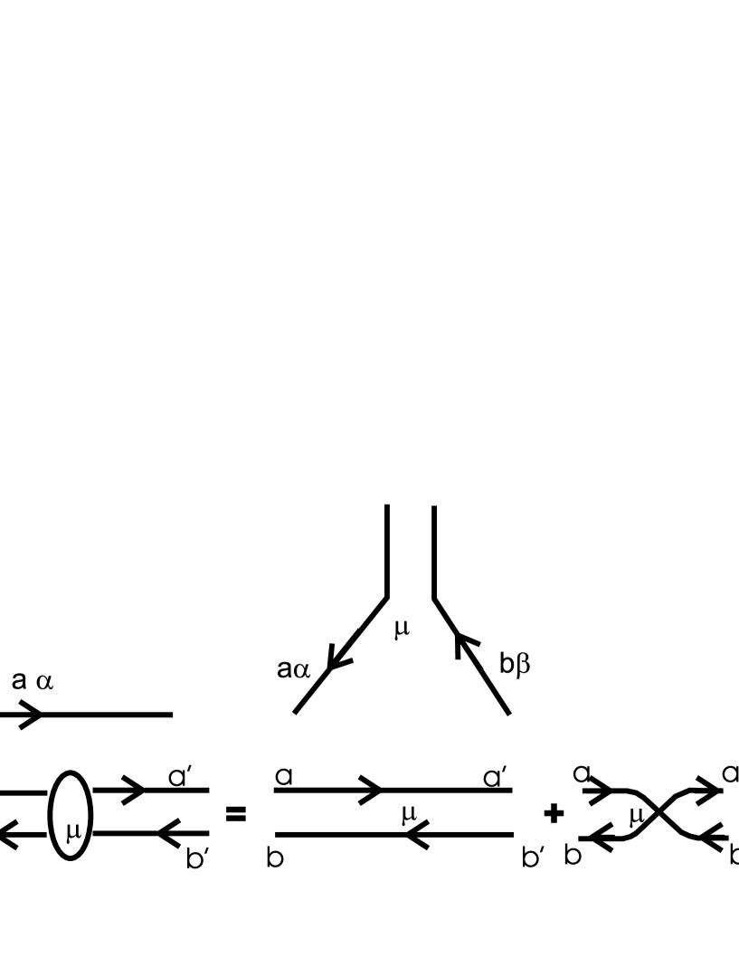
FIG. 1.: Single line electrons, double line bosons and the vertex in the $U(N,q)$ model

New, relative to the corresponding $SU(N)$ diagrams, is the presence of two terms in the boson propagator. Representing fermion propagators by oriented lines, boson double lines inherit an orientation from the electron lines that flow through a vertex. This inherited orientation, however, is not respected by the first term of the propagator in eq(21) and a consequence of this is illustrated in figure 2.

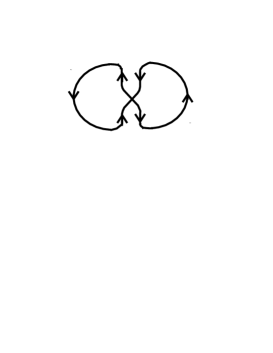
FIG. 2.: The boson propagator spoils the loop orientation

As in $SU(N)$ Yang Mills theory [3] or in the $SU(N)$ Hubbard model [4] a diagram can be viewed as a collection of index loops that are identified across double lines representing bosonic propagators. Each index loop spans a two dimensional area and in this way a topological surface gets associated with each diagram. By counting the number of vertices and index summations from each loop, we find that each diagram carries a weight (in powers of $N$) of

$$weight = N^{loops-\frac{S_{0}}{2}}=N^{S_{2}-\frac{S_{0}}{2}}\stackrel{{\scriptstyle S_{1}=\frac{3}{2}S_{0}}}{{=}}N^{\chi}$$

$$\chi = S_{2}-S_{1}+S_{0}$$

where $S_{2}$ is the number of loops or area like pieces, $S_{1}$ the number of propagators and $S_{0}$ the number of vertices and where $S_{1}=\frac{3}{2}S_{0}$ relates the number of propagators and vertices. In the present $U(N,q)$ extrapolation, non orientable surfaces contribute and a more general expression for the Euler characteristic must be used:

$\displaystyle\chi=2-2h-c-o$

Here $h$ stands for handles, $c$ for crosscaps and $o$ for openings (see e.g. [12] for a detailed discussion of the classification of surfaces). A ”crosscap” is the presence, in a loop, of a pair of  identified segments, that are traversed with the same orientation. For large $N$, diagrams of the disk topology $h=0=c$, $o=1$ dominate and these can be easily summed (the sums of the nonleading diagrams for $\chi=0$ and $\chi=-1$ are more complicated and will not be given here).

V Coupled integral equations for the leading graphs

Let us compute the electronic self energy to second order in perturbation theory:

$$\Sigma_{a_{1}\alpha_{1},b_{2}\beta_{2}}(1,2) = \frac{U}{3N}<T\left\{\left[z^{\mu}(1)\sigma^{\mu}\psi(1)\right]_{a_{1}\alpha_{1}}\left[\psi^{+}(2)\sigma^{\mu}z^{\mu}(2)\right]_{b_{2}\beta_{2}}\right\}>$$

$$= \frac{U}{3N}<T\left\{z_{a_{1}\alpha_{1}|b_{1}\beta_{1}}(1)z_{a_{2}\alpha_{2}|b_{2}\beta_{2}}(2)\right\}><T\left\{\psi(1)_{b_{1}\beta_{1}}\psi^{+}{}_{a_{2}\alpha_{2}}(2)\right\}>$$

with $z_{a\alpha|b\beta}\equiv z_{ab}^{\mu}\sigma_{\alpha\beta}^{\mu}$. From eq(45) of the appendix we find

$$\Sigma_{a_{1}\alpha_{1},b_{2}\beta_{2}}(1,2) \equiv \delta_{a_{1}b_{2}}\delta_{\alpha_{1}\beta_{2}}\sigma(1,2)$$

$$\sigma(1,2) = \frac{U(2N+1)}{3N}d(1,2)g(1,2)\stackrel{{\scriptstyle N\rightarrow\infty}}{{\rightarrow}}\frac{2U}{3}d(1,2)g(1,2)\text{ }$$

Strictly speaking, this is just lowest order perturbation theory. But to leading order in $N$ we get all the rainbow diagrams and these are summed by rendering the outermost rainbow explicit and we do indeed obtain the last equation with the full propagators (to leading order in $N$), but without vertex corrections (that are nonleading in $N$).  We now compute the self energy of the bosons to leading order (our notation was indicated in eq(21):

$$\Pi_{a_{1}b_{1}}^{\mu_{1}}|_{a_{2}b_{2}}^{\mu_{2}}(1,2)=\frac{U}{3N}<\left(\psi_{a_{1}\alpha_{1}}^{+}\sigma_{\alpha_{1}\beta_{1}}^{\mu_{1}}\psi_{b_{1}\beta_{1}}\right)(1)\cdot\left(\psi_{a_{2}\alpha_{2}}^{+}\sigma_{\alpha_{2}\beta_{2}}^{\mu_{2}}\psi_{b_{2}\beta_{2}}\right)(2)>$$ (25)

To lowest order this gives, upon using the invariant tensor properties of the fermion propagator

$$\Pi_{a_{1}b_{1}}^{\mu_{1}}|_{a_{2}b_{2}}^{\mu_{2}}(1,2) = \pi(1,2)\left(\text{\ }T^{\mu_{1}\mu_{2}}\right)_{a_{1}b_{1}a_{2}b_{2}}$$ (26)

$$\left(\text{\ }T^{\mu_{1}\mu_{2}}\right)_{a_{1}b_{1}a_{2}b_{2}} = \delta_{b_{1}a_{2}}\delta_{b_{2}a_{1}}\delta_{\mu_{1}\mu_{2}}(-1)^{\delta_{\mu 0}}$$ (27)

$$\pi(1,2) = -\frac{2U}{3N}G(1,2)G(2,1)$$ (28)

It is shown in eq (55) of the appendix that the conventional Dyson equation for the propagator leads to a corresponding scalar Dyson equation for $d$:

$\displaystyle d=\frac{1}{d_{0}^{-1}-\pi}$

The coupled integral equations

$$d = \frac{1}{d_{0}^{-1}-\pi}\text{ \ and\ \ \ }g=\frac{1}{g_{0}^{-1}-\sigma}$$ (29)

$$\sigma(1,2) = -\frac{\delta\Phi}{\delta g(2,1)}\text{ and }\pi(1,2)=\frac{2}{N}\frac{\delta\Phi}{\delta d(2,1)}$$ (30)

$$\Phi = -\frac{U}{3}g(1,2)d(1,2)g(2,1)$$ (31)

must be solved self consistently. Using the differential form of Dyson’s equations

$$\sigma(1,2) = -\frac{\delta}{\delta g(2,1)}Tr\left(\log g-g/g_{0}\right)$$ (32)

$$\pi(1,2) = -\frac{\delta}{\delta d(2,1)}Tr\left(\log d-d/d_{0}\right)$$ (33)

and eq(29) we find that the functional

$\displaystyle\Omega=\Phi+Tr\left(\log g-g/g_{0}\right)-\frac{N}{2}Tr\left(\log d-d/d_{0}\right)$

is stationary with respect to variations in $g$ and $d$. To understand the factor $\frac{N}{2}$, we note that the theory contains $2N$ complex fermions and $\sim 2N^{2}$ real bosons or $\frac{N}{2}$ times as many more complex bosons than fermions.

This leading generating functional is of the same form as a corresponding leading functional of the $SU(N)$ theory that was written down previously [4] which is consistent with a general idea that different groups have the same leading asymptotics, once their dimensions are taken large. Differences appear, however, at the first nonleading order, because of the nonorientable part of the boson propagator.

VI Conclusions

The main results of this paper are the following:

• we constructed an $U(N,q)$ extrapolation of the correlation problem that is dominated by planar diagrams at large $N$ and which permits pairing -

• the surfaces associated with the diagrams of this $U(N,q)$ theory now include non orientable ones -

• at the leading planar level, the integral equations and generating functional are of the same form as in the $SU(N)$ case.

It is very encouraging that the planar diagram approach to the correlation problem permits pairing, once an appropriate extrapolation is chosen. This is absolutely essential for its future use in investigating low temperature superconducting order in models of doped ceramics, organic conductors and other systems of interest. By using quaternion like objects, one has kept one of the crucial features of the electrons, their spinor character.

Regarding magnetic ordering, it is unclear at present whether antiferromagnetism at half filling will persist also for $N>1$ in this extrapolation. It is conceivable that the magnetization $\left(\psi^{+}L_{A}\psi\right)_{x}$, with $L_{A}$ a basis in the space of generators of $U(N,q)$, arranges itself to be antiparallel (in the sense of the metric $g_{AB}=TrL_{A}L_{B}^{+}$) at neighboring points $x$ on a bipartite lattice, in a similar fashion as discussed in [6].

It remains to find out, whether the small parameter 1/N introduced here is ”small enough” to confer predictive power to our approach. So far the only favorable indication we have is the overall agreement of the leading diagrams with those of FLEX plus the many interesting results obtained in this approximation [13]. If the present approach is successful, it will sharpen the FLEX method and a number of tough problems in the domaine of strongly correlated electrons will become transparent.

Acknowledgments

I am indebted to T. Dahm (Tuebingen) for continued correspondence on the FLEX approach, to members of Laboratoire de Chimie Quantique (Toulouse) and Theoretische Festkoerperphysik (Tuebingen) for lively discussions and useful comments, to G. Robert and A. Zvonkin (Bordeaux) for discussions on graphs and surfaces, to P. Sorba (Annecy) for comments on $U(N,q)$, to B. Bonnier for encouragement and to S.Villain-Guillot for a critical reading of the manuscript.

VII Appendix

A Calculation of $J_{ab}^{\mu}J_{ab}^{\mu}$

We use the definition $J_{ab}^{\mu}=\frac{1}{2}\left[\psi_{a\alpha}^{+}\sigma_{\alpha\beta}^{\mu}\psi_{b\beta}+h.c.\right]$ with $\sigma^{\mu}=\left\{i,\overrightarrow{\sigma}\right\}$ and calculate $J_{ab}^{\mu}J_{ab}^{\mu}$ in two steps via $J_{ab}^{\mu}J_{ab}^{\mu}=J_{ab}^{0}J_{ab}^{0}+\overrightarrow{J}_{ab}\overrightarrow{J}_{ab}$. First we determine $\sum J_{ab}^{0}J_{ab}^{0}:$

$$\sum J_{ab}^{0}J_{ab}^{0} = -\frac{1}{4}\sum\left[\psi_{a\tau}^{+}\psi_{b\tau}-\left(a\leftrightarrow b\right)\right]\left[\psi_{a\sigma}^{+}\psi_{b\sigma}-\left(a\leftrightarrow b\right)\right]$$ (34)

$$= \frac{1}{2}\sum-\left(\psi_{a}^{+}\psi_{b}\right)\left(\psi_{a}^{+}\psi_{b}\right)+\left(\psi_{b}^{+}\psi_{a}\right)\left(\psi_{a}^{+}\psi_{b}\right)$$ (35)

Second we determine $\sum\overrightarrow{J}_{ab}\overrightarrow{J}_{ab}:$

$$\sum\overrightarrow{J}_{ab}\overrightarrow{J}_{ab} = \sum\frac{1}{2}\psi_{a\alpha}^{+}\overrightarrow{\sigma}_{\alpha\beta}\psi_{b\beta}\left[\psi_{a\gamma}^{+}\overrightarrow{\sigma}_{\gamma\delta}\psi_{b\delta}+\left(a\leftrightarrow b\right)\right]$$ (36)

$$= \sum\frac{1}{2}\psi_{a\alpha}^{+}\psi_{b\beta}\left[\psi_{a\gamma}^{+}\psi_{b\delta}+\left(a\leftrightarrow b\right)\right]\left(2\delta_{\alpha\delta}\delta_{\beta\gamma}-\delta_{\alpha\beta}\delta_{\gamma\delta}\right)$$ (38)

$$\stackrel{{\scriptstyle\ast}}{{=}}\sum-\left(\psi_{a}^{+}\psi_{b}\right)\left(\psi_{a}^{+}\psi_{b}\right)-\left(\psi_{a}^{+}\psi_{a}\right)\left(\psi_{b}^{+}\psi_{b}\right)-\frac{1}{2}\left(\psi_{a}^{+}\psi_{b}\right)(\psi_{a}^{+}\psi_{b})-\frac{1}{2}\left(\psi_{a}^{+}\psi_{b}\right)(\psi_{b}^{+}\psi_{a})$$

The symbol $\stackrel{{\scriptstyle\ast}}{{=}}$ means modulo quadratic terms that correspond to an extra chemical potential. Combining eqs(34,36) we obtain

$$\sum J_{ab}^{0}J_{ab}^{0}+\overrightarrow{J}_{ab}\overrightarrow{J}_{ab}\stackrel{{\scriptstyle\ast}}{{=}}\sum-\left(\psi_{a}^{+}\psi_{a}\right)\left(\psi_{b}^{+}\psi_{b}\right)-2\left(\psi_{a}^{+}\psi_{b}\right)\left(\psi_{a}^{+}\psi_{b}\right)$$ (39)

Because there are only two spinor components we have $\left(\psi_{a}^{+}\psi_{b}\right)\left(\psi_{a}^{+}\psi_{b}\right)=-\frac{1}{2}\left(\psi_{a}^{+}\varepsilon\psi_{a}^{+}\right)\left(\psi_{b}\varepsilon\psi_{b}\right)$. Using this on eq(39) we find the required relation

$$\sum J_{ab}^{0}J_{ab}^{0}+\overrightarrow{J}_{ab}\overrightarrow{J}_{ab}=\sum\left(\psi_{a}^{+}\varepsilon\psi_{a}^{+}\right)(\psi_{b}\varepsilon\psi_{b})-\left(\psi_{a}^{+}\psi_{a}\right)\left(\psi_{b}^{+}\psi_{b}\right)\text{ + quadratic terms}$$ (40)

B Calculation of $<T\left\{\left[z(1)\psi(1)\right]_{a_{1}\alpha_{1}}\left[\psi^{+}(2)z(2)\right]_{b_{2}\beta_{2}}\right\}>$

It is convenient to organize the algebra as follows

$$<T\left\{\left[z(1)\psi(1)\right]_{a_{1}\alpha_{1}}\left[\psi^{+}(2)z(2)\right]_{b_{2}\beta_{2}}\right\}>=<T\left\{z_{a_{1}\alpha_{1}|b_{1}\beta_{1}}(1)z_{a_{2}\alpha_{2}|b_{2}\beta_{2}}(2)\right\}><T\left\{\psi(1)_{b_{1}\beta_{1}}\psi^{+}(2)_{a_{2}\alpha_{2}}\right\}>$$ (41)

$<T\left\{z(1)z(2)\right\}>$ is linearly related to $<T\left\{z_{a_{1}b_{1}}^{\mu_{1}}(1)z_{a_{2}b_{2}}^{\mu_{2}}(2)\right\}>$ for which we have an expression in eq(21) of the body of the paper:

$$< T\left\{z_{a_{1}\alpha_{1}|b_{1}\beta_{1}}(1)z_{a_{2}\alpha_{2}|b_{2}\beta_{2}}(2)\right\}>=\sum_{\mu}\sigma_{\alpha_{1}\beta_{1}}^{\mu}\sigma_{\alpha_{2}\beta_{2}}^{\mu}<T\left\{z_{a_{1}b_{1}}^{\mu}(1)z_{a_{2}b_{2}}^{\mu}(2)\right\}>$$ (42)

$$= \sum_{\mu}\sigma_{\alpha_{1}\beta_{1}}^{\mu}\sigma_{\alpha_{2}\beta_{2}}^{\mu}\cdot d(1,2)\cdot\frac{1}{2}\left[\delta_{a_{1},a_{2}}\delta_{b_{1},b_{2}}+(-1)^{\delta_{\mu,0}}\delta_{a_{1},b_{2}}\delta_{b_{1},a_{2}}\right]$$ (43)

$$= d(1,2)\delta_{a_{1},a_{2}}\delta_{b_{1},b_{2}}\cdot\frac{1}{2}\sigma_{\alpha_{1}\beta_{1}}^{\mu}\sigma_{\alpha_{2}\beta_{2}}^{\mu}+d(1,2)\delta_{a_{1},b_{2}}\delta_{b_{1},a_{2}}\cdot\frac{(-1)^{\delta_{\mu,0}}}{2}\sigma_{\alpha_{1}\beta_{1}}^{\mu}\sigma_{\alpha_{2}\beta_{2}}^{\mu}$$ (44)

with $\sigma^{\mu}=\{i,\overrightarrow{\sigma}\}$. We use the relations $\frac{1}{2}\sigma_{\alpha_{1}\beta_{1}}^{\mu}\sigma_{\alpha_{2}\beta_{2}}^{\mu}=-\varepsilon_{\alpha_{1}\alpha_{2}}\varepsilon_{\beta_{1}\beta_{2}}$ and $\frac{1}{2}\sigma_{\alpha_{1}\beta_{1}}^{\mu}\sigma_{\alpha_{2}\beta_{2}}^{\mu}(-1)^{\delta_{\mu,0}}=\delta_{\alpha_{1}\beta_{2}}\delta_{\beta_{1}\alpha_{2}}$ in eq(42) to obtain:

$\displaystyle<T\left\{z_{a_{1}\alpha_{1}|b_{1}\beta_{1}}(1)z_{a_{2}\alpha_{2}|b_{2}\beta_{2}}(2)\right\}>=d(1,2)\left(\delta_{a_{1},b_{2}}\delta_{\alpha_{1}\beta_{2}}\cdot\delta_{b_{1},a_{2}}\delta_{\beta_{1}\alpha_{2}}-\delta_{a_{1},a_{2}}\varepsilon_{\alpha_{1}\alpha_{2}}\cdot\delta_{b_{1},b_{2}}\varepsilon_{\beta_{1}\beta_{2}}\right)$

where we recognize the basic invariant tensors of the group $U(N,q)$. Invoking the tensor character of the fermion propagator in eq(21) , the expression in eq(41) reduces to

$$< T\left\{z_{a_{1}\alpha_{1}|b_{1}\beta_{1}}(1)z_{a_{2}\alpha_{2}|b_{2}\beta_{2}}(2)\right\}><T\left\{\psi(1)_{b_{2}\beta_{1}}\psi^{+}(2)_{a_{2}\alpha_{2}}\right\}>$$ (45)

$$= d(1,2)\left(\delta_{a_{1},b_{2}}\delta_{\alpha_{1}\beta_{2}}\cdot\delta_{b_{1},a_{2}}\delta_{\beta_{1}\alpha_{2}}-\delta_{a_{1},a_{2}}\varepsilon_{\alpha_{1}\alpha_{2}}\cdot\delta_{b_{1},b_{2}}\varepsilon_{\beta_{1}\beta_{2}}\right)\cdot g(1,2)\delta_{b_{1}a_{2}}\delta_{\beta_{1}\alpha_{2}}$$ (46)

$$= d(1,2)g(1,2)\left(2N+1\right)\delta_{a_{1},b_{2}}\delta_{\alpha_{1}\beta_{2}}$$ (47)

which is the desired expression.

C Scalar form of the bosonic Dyson equation

It remains to see how this self energy modifies the scalar coefficient $D(1,2)$. We must evaluate the sum

$$D=D_{0}+D_{0}\Pi D_{0}+...=D_{0}\sum\left(\Pi D_{0}\right)^{n}=D_{0}\frac{1}{1-\Pi D_{0}}\stackrel{{\scriptstyle??}}{{=}}\frac{1}{D_{0}^{-1}-\Pi}$$ (48)

$D_{0}$ is proportional to a projector $P$ onto matrices of definite symmetry type, its inverse $D_{0}^{-1}$ does not exist and, at first glance, Dyson’s equation appears ill defined. In any case we need a Dyson type equation for the scalar quantity $d$ that encapsulates the information of $D$. The quantities entering the series in eq(48) are

$$D(1,2) = \delta_{\mu_{1},\mu_{2}}d(1,2)P^{\mu}\text{ \ \ \ \ \ \ \ \ \ \ \ \ \ ''projection''}$$ (49)

$$\Pi^{\mu_{1},\mu_{2}} = \pi(1,2)\delta_{\mu_{1}\mu_{2}}(-1)^{\delta_{\mu 0}}T^{\mu}\text{ \ \ \ ''transposition''}$$ (50)

with $$:$$ (51)

$$P^{\mu}\text{ } = \frac{1}{2}\left[\delta_{a_{1},a_{2}}\delta_{b_{1},b_{2}}+(-1)^{\delta_{\mu,0}}\delta_{a_{1},b_{2}}\delta_{b_{1},a_{2}}\right]$$ (52)

$$T^{\mu} = (-1)^{\delta_{\mu 0}}\delta_{b_{1}a_{2}}\delta_{b_{2}a_{1}}\text{ ''transposition''}$$ (53)

Our definitions were chosen so that the matrices are contracted with each other in the same order as one writes them. The relations

$$T^{\mu}P^{\mu}=P^{\mu}T^{\mu}$$ (54)

come as no surprise and they mean that the operator $\Pi^{\mu_{1},\mu_{2}}$ acts as a multiplication by the scalar $\pi(1,2)$. We can now sum up the series eq(48)

$$D = D_{0}+D_{0}\Pi D_{0}+...=Pd_{0}\sum_{n=0..\infty}\left(\pi d_{0}\right)^{n}=Pd_{0}\frac{1}{1-\pi d_{0}}=\frac{P}{d_{0}^{-1}-\pi}$$ (55)

$$\rightarrow d^{-1}=d_{0}^{-1}-\pi$$ (56)

where $\left(\pi d_{0}\right)^{n}$ is meant in the sense of convolutions and the last equation is the desired scalar Dyson equation.

REFERENCES

- [1] J. Hubbard, Proc. Roy. Soc London A 276 (1963) and A 281 (1964) 401.
- [2] P. Fulde, ”Electron Correlations in Molecules and Solids”, Springer Series in Solid-State Sciences 100, Springer, Berlin, 1991; F. Gebhardt, ” The Mott Metal-Insulator Transition”, Springer, N.Y. 1997.
- [3] G. ’t Hooft, Nucl. Phys. B72 (1974) 461 and Nucl. Phys. B75 (1974) 461.
- [4] ”Planar diagram approach to the correlation problem”, cond-mat/9912350, to appear in Phys. Rev. B.
- [5] N. E. Bickers and D. J. Scalapino, Ann. Phys. (N. Y.) 193 (1989) 206.
- [6] N. Read and S. Sachdev, Phys. Rev. Lett. 66, (1991)17773.
- [7] M. Vojta, S. Sachdev, Phys.Rev. Lett. 83 (1999) 3916.
- [8] C. Chevalley, ”The Theory of Lie Groups”, Princeton University Press, Princeton 1946
- [9] A. A. Abrikosov, L. P. Gorkov and I. E. Dzyaloshinski, ”Methods of Quantum Field Theory in Statistical Mechanics, Dover, N. Y. 1997.
- [10] There is no complication due to an extra trace piece as there was in the extrapolation
- [11] G. Baym, Phys. Rev. B 127 (1962) 1391; J. M. Luttinger and J. C. Ward, Phys. Rev. 118 (1960) 1417.
- [12] J. Stillwell, ”Classical Topology and Combinatorial Group Theory”, Graduate Texts in Mathematics 72, Springer, N.Y. 1993.
- [13] For Flex applied to more realistic models, see for example G. Esirgen, H.-B. Schuettler, N. E. Bickers, Phys. Rev. Lett.82(1999)1217; for aplications to organic superconductors: H. Kino, H. Kontani, cond-mat 9905054; for marginal fermion behavior: T. Dahm, L. Tewordt, Phys. Rev. B52 (1995)1297.