Andreev scattering and Josephson current in a one-dimensional electron liquid

Abstract

Andreev scattering and the Josephson current through a one-dimensional interacting electron liquid sandwiched between two superconductors are re-examined. We first present some apparently new results on the non-interacting case by studying an exactly solvable tight-binding model rather than the usual continuum model. We show that perfect Andreev scattering (i.e. zero normal scattering) at the Fermi energy can only be achieved by fine-tuning junction parameters, a fine-tuning which is possible even with bandwidth mismatch between superconductor and normal metal. We also obtain exact results for the Josephson current, which is generally a smooth function of the superconducting phase difference except when the junction parameters are adjusted to give perfect Andreev scattering, in which case it becomes a sawtooth function. We then observe that, even when interactions are included, all low energy properties of a junction ($E<<\Delta$, the superconducting gap) can be obtained by “integrating out” the superconducting electrons to obtain an effective Hamiltonian describing the metallic electrons only with a boundary pairing interaction. This boundary model provides a suitable starting point for bosonization/renormalization group/boundary conformal field theory analysis. We argue that total normal reflection and total Andreev reflection correspond to two fixed points of the boundary renormalization group. For repulsive bulk interactions the Andreev fixed point is unstable and the normal one stable. However, the reverse is true for attractive interactions. This implies that a generic junction Hamiltonian (without fine-tuned junction parameters) will renormalize to the normal fixed point for repulsive interactions but to the Andreev one for attractive interactions. An exact mapping of our tight-binding model to the Hubbard model with a transverse magnetic field is used to help understand this behavior. We calculate the critical exponents, which are different at these two different fixed points.

I introduction

One of the fascinating consequences of superconductivity is the phenomenon of Andreev scattering at a normal metal/superconductor (NS) junction. This corresponds to an incoming electron from the normal side being reflected back as a hole, thereby producing an additional Cooper pair in the superconductor condensate. Both normal and Andreev reflections are expected to occur in a realistic NS junction, in addition to quasiparticle transmission into the superconductor. If the gap is large enough, the latter’s propagation is suppressed and squared reflection amplitudes add up to one through probability current conservation. Building up on Andreev reflection, one arrives at the related phenomenon of the Josephson current, in which the normal region of an SNS junctions carries a supercurrent driven by the gap phase difference between left and right superconductors.

While the original work in this field[1, 2, 3, 4] treated the normal metal within the Fermi liquid framework (i.e. essentially ignored interactions), the effect of interactions for the case of a one-dimensional metal between two superconductors has been treated recently by several groups[5, 6, 7, 8] using bosonization and renormalization group methods. The methods and conclusions of these works are closely related to previous work on tunnelling through a single impurity in a quantum wire.[9]

We have chosen to re-examine this subject in both non-interacting and interacting cases because we feel that previous treatments have missed some interesting physics. In particular, most of the standard work on the non-interacting case has essentially ignored band structure effects, using a free electron model with a pairing potential that varies abruptly accross the junction, together with a scattering potential at the interface. A more recent paper[10] considers the case where the Fermi velocity is different on the S and N side. The conclusion of this work is that, at the Fermi energy, there is perfect Andreev reflection (and therefore 0 normal reflection) when the scattering potential and velocity mismatch are absent. Both of these effects serve to increase the normal scattering amplitude in an additive way. We arrive at qualitatively different conclusions by explicitly including band structure in the form of an exactly solveable one-dimensional tight-binding model with Hamiltonian:

$$H-\mu N=\sum_{j}\left[(-t_{j,j+1}\psi_{j\sigma}^{\dagger}\psi_{j+1\sigma}+\Delta_{j}\psi_{j\uparrow}^{\dagger}\psi_{j\downarrow}^{\dagger}+h.c.)+(V_{j}-\mu)\psi_{j\sigma}^{\dagger}\psi_{j\sigma}\right].$$ (1)

The chemical potential, $\mu$, is assumed to lie within the band on the normal side $|\mu|<2t$ and $h.c.$ stands for Hermitean conjugate. Here the interface is chosen to lie between sites 0 and 1 with the superconductor on the negative $x$-axis and the normal metal on the positive $x$ axis so that:

$$t_{j,j+1}=\left\{\begin{array}[]{ll}t&j>0\\ t^{\prime\prime}&j=0\\ t^{\prime}&j<0\end{array}\right.,$$ (5)

$$V_{j}=V\delta_{j1},\hskip 28.45274pt\Delta_{j}=\left\{\begin{array}[]{ll}\Delta&j\leq 0\\ 0&j>0\end{array}\right..$$ (8)

$\Delta_{j}$ represents the pairing interaction which exists on the superconducting side ($j\leq 0$) only. For simplicity we consider both normal and superconducting sides to be one-dimensional, but see below. The notion of a “perfect junction” becomes less clear in such a model. In the particle-hole symmetric case, $\mu=V=0$, we find that there is always some normal scattering at the Fermi energy unless the interface tunnelling parameter, $t^{\prime\prime}$, is fine-tuned to a particular value. In the limit $|\Delta|<<t,t^{\prime}$, this particular value becomes

$$t^{\prime\prime}=\sqrt{tt^{\prime}}.$$ (9)

For general values of the chemical potential we find that both $t^{\prime\prime}$ and the normal scattering intensity, $V$, must be fine-tuned in order to achieve perfect Andreev reflection. We emphasise that these conclusions seem to be different than the previous ones obtained without explicit consideration of band effects. For example, in the particle-hole symmetric case it is possible to get perfect Andreev reflection even with Fermi velocity mismatch ($t\neq t^{\prime}$) provided that $t^{\prime\prime}$ is adjusted to the right value. It is worth emphasizing that the case of infinite interface tunnelling: $t^{\prime\prime}>>t,t^{\prime}$ does not correspond to perfect Andreev reflection as one might naively suppose, but instead to zero Andreev reflection. The physical reason is that, in this limit, two electrons get trapped at the interface on sites 0 and 1, effectively decoupling all sites with $j<0$ from all sites with $j>1$. In this limit the normal side does not “feel” the pairing and hence exhibits no Andreev reflection.

We are not aware of any previous explicit calculation of the Josephson current for such an interface model which we perform here. We consider two, possibly different, interfaces separated by a distance of $l$ lattice sites with the pairing potentials having a phase difference $\chi$. The (zero temperature) Josephson current is defined from the derivative of the groundstate energy with respect to this phase difference:

$$I(\chi)=2e\frac{d}{d\chi}E_{0}.$$ (10)

While the groundstate energy is obtained by summing over all states below the Fermi surface, we show explicitly that its derivative with respect to $\chi$ only depends on quantities defined at the Fermi surface, being insensitive to the details of the band structure. When the junction parameters are fine-tuned to give perfect Andreev reflection we find that the Josephson current is a sawtooth function of $\chi$:

$$I(\chi)\to\frac{ev_{f}}{\pi l}\chi,\hskip 28.45274pt(\hbox{mod}\ 2\pi),$$ (11)

with steps of size $2ev_{f}/l$ occurring at $\chi=(2n+1)\pi$. For any other choice of junction parameters the Josephson current is a smooth function of $\chi$. For example, in the limit of a weak junction, $t^{\prime\prime}<<t,t^{\prime}$, we find:

$$I(\chi)\propto(t^{\prime\prime})^{4}\sin\chi.$$ (12)

While these formulas are well-known results, our method in fact allows us to calculate exactly the zero-temperature Josephson current in the general case of arbitrary amounts of normal versus Andreev reflection, independently at each boundary. The full crossover between the above two limits is thus described.

One approach which we shall make much use of in this paper is that of an effective field theory, whereby the superconducting side is replaced by a particular boundary contribution on the normal side. There are several reasons why it is convenient to “integrate out” the electrons on the superconducting side of the junction in such a way as to obtain an effective Hamiltonian for the electrons on the normal side. This is a very natural thing to do considering the fact that the superconducting electrons have a gap in their spectrum: if we consider physics at energy scales small compared to the gap we expect to obtain a simple effective action without any retarded interactions. (This may break down for non s-wave pairing where the gap vanishes in certain directions; we do not consider that case here.) The resulting effective Hamiltonian (for a single junction) is:

$$H-\mu N=-t\sum_{j\geq 1}\left[(\psi_{j\sigma}^{\dagger}\psi_{j+1\sigma}+h.c.)-\mu\psi^{\dagger}_{j\sigma}\psi_{j\sigma}\right]+\left[\Delta_{B}\psi^{\dagger}_{1,\uparrow}\psi^{\dagger}_{1,\downarrow}+h.c.\right]+V_{B}\psi^{\dagger}_{1\sigma}\psi_{1\sigma}.$$ (13)

The effective boundary pairing interaction, $\Delta_{B}$ and effective boundary scattering potential, $V_{B}$, depend on all the parameters of the superconductor and the junction, $t^{\prime}$, $\Delta$, $t^{\prime\prime}$ , $V$. Beginning from our interface model of Eq. (1) we determine explicitly the parameters $\Delta_{B}$ and $V_{B}$ of the boundary model and check that low energy properties are faithfully reproduced. Of course, we again find with the boundary pairing model that perfect Andreev reflection only occurs if the boundary parameters are fine-tuned. In particular, for the particle-hole symmetric case, $\mu=V_{B}=0$, the condition is:

$$|\Delta_{B}|=t.$$ (14)

Note that is is not $\Delta_{B}\to\infty$ as one might naively suppose.

One advantage of the boundary model is that it should arise from much more general, and more realistic, interface models. While the simple form of Eq. (1), quadratic in fermion operators, is the result of a mean field approximation to a more realistic model with pairing or electron-phonon interactions on the superconducting side, we expect that the effective Hamiltonian of Eq. (13) will still be valid at energies small compared to the gap when the interactions on the superconducting side are treated more accurately. Furthermore, it is more or less obvious that the same effective Hamiltonian arises when the one-dimensional normal metal is coupled to a three-dimensional superconductor. This is an important generalization since superconductivity is not believed to occur in a strictly one-dimensional system.

More generally we wish to add interactions to our Hamiltonian on the normal side which we assume to be one-dimensional. A simple choice would be an onsite (Hubbard) interaction for all sites $j\geq 1$:

$$H \to H+H_{int}$$ (15)

$$H_{int} = {U\over 2}\sum_{j\geq 1}(n_{j}-1)^{2},$$ (16)

where $n_{j}$ is the total electron number operator at site $j$. We could also consider longer range density-density interactions. We will be interested in the case of both repulsive and attractive bulk interactions; the latter may arise in a low energy effective theory from phonon exchange. The negative $U$ Hubbard model has a gap for spin excitations which can be eliminated by considering longer range interactions. We will discuss both cases with zero and non-zero spin gap. These interactions can be treated essentially exactly, at low energies, using bosonization, renormalization group and conformal field theory techniques. It is a major purpose of this paper to discuss how to generalize these techniques to the interface model. We argue that this is best done by integrating out the superconducting electrons to obtain the boundary model of Eq. (13) with the bulk interactions, $H_{int}$ added. (More generally, we might also obtain additional interactions at the boundary. These can be treated in the same framework.) Indeed, this approach seems to be more or less forced upon us by the renormalization group philosophy of integrating out high energy modes to obtain an effective low energy Hamiltonian. Having performed the initial step of integrating out the gapped degrees of freedom on the superconducting side we may then proceed to analyse the effective Hamiltonian with bulk and boundary terms using general methods developed to deal with quantum impurity problems.[11] Of course, our results will only be valid at energies $E<<\Delta$.

The boundary renormalization group approach leads to the conclusion that the boundary interactions will renormalize to a fixed point corresponding to a conformally invariant boundary condition. It appears likely that there are only two such boundary conditions that occur in this problem, in the particle-hole symmetric case ($\mu=V=V_{B}=0$) corresponding to a free boundary condition (b.c.), $\Delta_{B}=0$ which preserves electron number and therefore has no Andreev reflection and to an “Andreev boundary condition” for which there is perfect Andreev reflection. Which of these boundary conditions is stable under renormalization group transformations depends on the sign of the bulk interactions, $U$. We find that the free b.c. is stable for repulsive bulk interactions but the Andreev b.c. is stable for attractive bulk interactions ($U<0$). We calculate the various critical exponents associated with these critical points. It is important to realize that critical exponents are characteristic of a particular fixed point and are different at the free and Andreev fixed points. Thus, for instance with repulsive bulk interactions, if we started with bare interface parameters that put the interface close to the Andreev fixed point then the exponents characterizing the initial flow away from the Andreev fixed point at high temperature are different than the exponents characterizing the flow towards the free fixed point at low temperature. However, it should be emphasized that for a generic choice of bare interface parameters the Hamiltonian will not be near the Andreev fixed point; this requires fine-tuning. The situation is similar in the non particle-hole symmetric case except we now get lines of fixed points with either $0$ or perfect Andreev reflection.

The first work that we are aware of on Andreev scattering in Tomonaga-Luttinger liquids[5] attempted to apply boundary RG techniques without explicitly intergrating out the superconducting side and without taking into account the effect of the b.c.’s on the exponents. This led to incorrect predictions for the exponent governing the Josephson current. [[6]] used a method closely related to ours but applied it to a different geometry: a closed normal ring in contact with superconductors at two points. Takane[7] corrected some of the earlier result in [[5]] for the exponent governing the Josephson current using methods essentially equivalent to ours but without explicitly invoking the concept of integrating out the superconducting side. We extend Takane’s result by introducing the conceptually important and very useful notion of integrating out the superconducting electrons thus making clear the relationship between the interface problem, other quantum impurity problems and boundary conformal field theory. This facilitates a more general discussion of the universal critical behaviour. In particular we discuss the behaviour of the Josephson current in the vicinity of the Andreev fixed point, obtaining quite different results than those in [[5]], and discussing how the functional dependence of the current on the superconducting phase difference crosses over between sawtooth and smooth forms.

Given the difficulty of achieving perfect Andreev scattering in the non-interacting case our conclusion is quite remarkable that, with attractive bulk interactions, a generic interface will renormalize to perfect Andreev scattering as $T\to 0$. It must be admitted that this conclusion is based on an unproven but widely made assumption about RG flows and fixed points in the boundary sine-Gordon model which arises here after bosonization. In order to make some of our rather unintuitive results seem more plausible we discuss an exact mapping of our boundary pairing model (in the particle-hole symmetric case) into a Hubbard model with a bulk magnetic field and a transverse boundary magnetic field. In the transformed model the Andreev boundary condition corresponds to one in which the boundary electron has a frozen transverse spin polarization.

In the next section we give the solution of the interface and boundary models and discuss their equivalence, in the case of zero bulk interactions. Most of the details of the equivalence are relegated to an appendix. In Sec. III we consider an $S_{1}NS_{2}$ system and calculate the Josephson current. In Sec. IV we include bulk interactions in the boundary model and determine phase diagrams and critical exponents. In Sec. V we discuss the exact mapping onto the Hubbard model with bulk and boundary magnetic fields.

II The lattice interface and boundary models

In this section, we consider various lattice models of normal metal-superconductor contacts in the case of zero bulk interactions. The generic Hamiltonian for all of these will be (1), with various geometries, sets of hopping strenths, and potentials specified along the way. The calculation procedure is similar to the usual one used in dealing with continuum models: the wavefunctions are found for each sector, and the matching conditions at the contacts yield consistency equations from which the various reflection/transmission coefficients are obtained.

We start by performing the Bogoliubov-de Gennes transformation

$$\psi_{j\sigma}=\sum_{\alpha}[u_{\alpha j}\gamma_{\alpha\sigma}-\sigma v^{*}_{\alpha j}\gamma^{\dagger}_{\alpha-\sigma}],$$ (17)

where the quasiparticle operators satisfy $\{\gamma_{\alpha\sigma},\gamma^{\dagger}_{\alpha^{\prime}\sigma^{\prime}}\}=\delta_{\alpha\alpha^{\prime}}\delta_{\sigma\sigma^{\prime}}$ and $\alpha$ is a (real) quasimomentum index. We obtain [2], by requiring the Hamiltonian to be diagonal $(H=E_{0}+\sum_{\alpha}\epsilon_{\alpha}\gamma_{\alpha\sigma}^{\dagger}\gamma_{\alpha\sigma})$ the following lattice Bogoliubov-de Gennes equations:

$$\epsilon_{\alpha}u_{\alpha j} = -t_{jj-1}u_{\alpha j-1}-t_{jj+1}u_{\alpha j+1}+(V_{j}-\mu)u_{\alpha j}+\Delta_{j}v_{\alpha j}$$ (18)

$$\epsilon_{\alpha}v_{\alpha j} = t_{jj-1}v_{\alpha j-1}+t_{jj+1}v_{\alpha j+1}-(V_{j}-\mu)v_{\alpha j}+\Delta^{*}_{j}u_{\alpha j}.$$ (19)

The solutions of these equations in two particular geometries are presented below. The emphasis is put on the calculation of the Andreev reflection coefficient and on the low-energy properties of the system.

A The lattice interface model

As a simple toy model for a NS interface, we consider the geometry depicted in figure 1. This tight-binding model is one of free electrons in which a nonvanishing superconducting order parameter has been induced by an unspecified mechanism on the left-hand sites of the lattice only. Although it is a straightforward lattice version of the ubiquitous continuum one-dimensional models used in [[4]] and numerous subsequent work, let us underline that our model includes some additional features, namely different bandwidths $t,t^{\prime}$ on the normal and superconducting sides, and an arbitrary coupling $t^{\prime\prime}$ together with a local scattering potential $V$ at the interface. In other words, our lattice interface model is defined by the BdG equations (19) with the choice of parameters in (8).

FIG. 1.: The interface model. Dots represent lattice sites, labeled by integers. On the left is the superconductor, with gap $\Delta$ and bandwidth $t^{\prime}$. It is coupled to a normal metal with bandwidth $t$ through a junction of strength $t^{\prime\prime}$, with a local potential $V$ to tune the normal scattering rate at the contact.

The calculation of the normal and Andreev reflection coefficients in the lattice interface model is nothing but an exercise in elementary quantum mechanics. Namely, it is performed by choosing an appropriate ansatz for the wavefunctions, after which solving for the matching conditions of the eigenstates at the interface yields all the desired information.

Let us implement this procedure by taking a simple travelling wave solution to the Bogoliubov-de Gennes equations (19):

$$u_{\alpha j}=\left\{\begin{array}[]{ll}e^{-i\alpha j}+R_{N}e^{i\alpha j}&j\geq 1\\ T_{N}e^{-i\beta j}+(-1)^{j}T_{N}^{\prime}e^{-i\delta j}&j\leq 0\end{array}\right.\hskip 28.45274ptv_{\alpha j}=\left\{\begin{array}[]{ll}(-1)^{j}R_{A}e^{i\gamma j}&j\geq 1\\ T_{A}e^{-i\beta j}+(-1)^{j}T_{A}^{\prime}e^{-i\delta j}&j\leq 0\end{array}\right..$$ (24)

In the above equation, the quasimomenta $\beta$ and $\delta$ will turn out to be complex for the region of parameters we will be concentrating on, namely at energies below the superconducting gap. This means that the wavefunction amplitudes $u_{\alpha j}$ and $v_{\alpha j}$ are exponentially decaying on the left-hand side.

The rest of the procedure is then a simple matter of substituting (24) in (19) and carrying out the necessary algebra. The energy is

$$\epsilon_{\alpha}=-2t\cos\alpha-\mu,$$ (25)

while the other parameters in (24) are given by

$$\cos\gamma=\cos{\alpha}+\mu/t,\hskip 28.45274pt2t^{\prime}\cos{\beta} = \sqrt{(2t\cos{\alpha}+\mu)^{2}-|\Delta|^{2}}-\mu,$$ (26)

$$2t^{\prime}\cos{\delta} = \sqrt{(2t\cos{\alpha}+\mu)^{2}-|\Delta|^{2}}+\mu.$$ (27)

Although all reflection and transmission coefficients can be calculated explicitly, a simpler form for these expressions is obtained if we are interested primarily in the scattering of particles whose energy is very small compared to the superconducting energy gap. The $\epsilon\rightarrow 0$ limit gives

$$\cos{\alpha}=-\cos{\gamma}=-\frac{\mu}{2t}, \sin{\alpha}=\sin{\gamma}=\sqrt{1-\mu^{2}/{4t^{2}}},$$ (28)

$$\cos{\beta}=-(\cos{\delta})^{*}=-i|\Delta|/{2t^{\prime}}-\mu/{2t^{\prime}},\hskip 28.45274pt \sin{\beta}=(\sin{\delta})^{*}=\sqrt{1-(i|\Delta|+\mu)^{2}/{4{t^{\prime}}^{2}}},$$ (29)

and allows us to write the following expression for the Andreev reflection coefficient:

$$R_{A}|_{\epsilon=0}=ie^{-i\chi}\frac{t{t^{\prime\prime}}^{2}}{t^{\prime}}\frac{\sqrt{1-\mu^{2}/4t^{2}}\left[-\frac{|\Delta|}{t^{\prime}}+\sin\beta+\sin\delta\right]}{t^{2}-\mu^{2}/4+(V-\mu/2-\frac{{t^{\prime\prime}}^{2}}{t^{\prime}}e^{i\beta})(V-\mu/2+\frac{{t^{\prime\prime}}^{2}}{t^{\prime}}e^{i\delta})}.$$ (30)

In the above, $\chi$ is the phase of the order parameter, $\Delta=|\Delta|e^{i\chi}$. Note that the reflection coefficients moreover obey the sum rule $|R_{A}|^{2}+|R_{N}|^{2}=1$ at half-filling, in view of the conservation of the current $t_{jj+1}[u^{*}_{\alpha j+1}u_{\alpha j}-v^{*}_{\alpha j+1}v_{\alpha j}-h.c.]$.

This low-energy Andreev reflection coefficient, as a function of the bandwidths $t,t^{\prime}$ and of the strength of the pairing $\Delta$, as well as of the tunneling strength $t^{\prime\prime}$ and local scattering potential $V$, obeys some simple but interesting properties. Imagining for example a generic experimental setup in which variations in $t^{\prime\prime}$ and $V$ can be implemented, we can ask how $R_{A}|_{\epsilon=0}$ behaves. A simple variation yields that the optimal amplitude is achieved for

$$V_{max}=\frac{\mu}{2}+\frac{{t^{\prime\prime}}^{2}}{2t^{\prime}}(e^{i\beta}+c.c.).$$ (31)

(Here $c.c.$ denotes complex conjugate.) Subsequently tuning $t^{\prime\prime}$ yields a maximum at

$${t^{\prime\prime}}_{max}^{2}=2tt^{\prime}\frac{\sqrt{1-\mu^{2}/4t^{2}}}{-\frac{|\Delta|}{t^{\prime}}+(\sin\beta+c.c.)}.$$ (32)

In the particle-hole symmetric case, this simplifies to

$${t^{\prime\prime}}_{max}^{2}=tt^{\prime}\left[\sqrt{1+\frac{|\Delta|^{2}}{4{t^{\prime}}^{2}}}+\frac{|\Delta|}{2t^{\prime}}\right].$$ (33)

Tuning the parameters in such a way, we find perfect Andreev reflection, i.e.

$$R_{A}{|_{\epsilon=0,V_{max},t^{\prime\prime}_{max}}}=ie^{-i\chi}$$ (34)

In terms of left- and right-movers in the continuum limit of (24), defined in Sec. IV, this corresponds to

$$\Psi_{R\uparrow}(0)=-ie^{i\chi}\Psi_{L\downarrow}^{\dagger}(0),\hskip 28.45274pt\Psi_{R\downarrow}(0)=ie^{i\chi}\Psi_{L\uparrow}^{\dagger}(0),$$ (35)

which are simply the perfect Andreev conditions usually imposed.

Thus, pure Andreev boundary conditions are obtainable in the lattice interface model by simply tuning two parameters in the general non particle-hole symmetric case. For the particle-hole symmetric case, it is enough to tune one parameter.

B The lattice boundary model

At energies below the superconducting gap, all wavefunctions incident on the NS interface from the normal side are eventually reflected back through either normal or Andreev reflection processes. The vanishing of the transmission coefficients opens the door to the formulation of a different approach than that adopted in the interface model, namely one in which we consider a system with a boundary obtained by “integrating out” the superconducting side, yielding an effective pairing potential localized at the original contact. In all generality, we will also consider a potential present at the boundary.

What we could call the lattice boundary model can be directly defined through the BdG equations (19), but our system (illustrated in figure 2) is now taken to live on the axis of positive integers, with a boundary at $j=0$ having on-site pairing $\Delta_{B}$ and potential $V_{B}$ on the first site. The hopping strength is taken to be $t$ between all sites. For the moment, we will perform all the relevant calculations from scratch, deferring the explicit connection with the previous interface model until later.

FIG. 2.: The boundary model. The superconductor has been replaced by effective boundary potentials $\Delta_{B}$ and $V_{B}$.

In the same way as for the interface model, we can calculate the normal and Andreev reflection coefficients by simple quantum mechanics. Of primary interest is the Andreev one, which is readily obtained by using the ansatz

$$u_{\alpha j}=e^{-i\alpha j}+R_{N}e^{i\alpha j},\hskip 14.22636ptv_{\alpha j}=(-1)^{j}R_{A}e^{i\gamma j}$$ (36)

in the lattice BdG equations (19) in the geometry just described. We find again $\epsilon_{\alpha}=-2t\cos\alpha-\mu$ with $\cos\gamma=\cos\alpha+\mu/t$, together with

$$R_{A}=2i\frac{\Delta^{*}_{B}t\sin{\alpha}}{|\Delta_{B}|^{2}+(te^{-i\alpha}+V_{B})(-te^{-i\gamma}+V_{B})}$$ (37)

which, at zero energy, becomes

$$R_{A}|_{\epsilon=0}=2i\frac{\Delta^{*}_{B}t\sqrt{1-\mu^{2}/4t^{2}}}{|\Delta_{B}|^{2}+V_{B}(V_{B}-\mu)+t^{2}}.$$ (38)

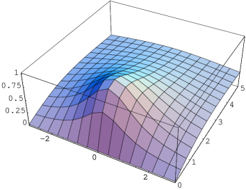
FIG. 3.: $|R_{A}|$ for the boundary model at half-filling, plotted over the range $0\leq|\Delta_{B}|/t\leq 5$ and $-3\leq V_{B}/t\leq 3$.

FIG. 4.: $|R_{A}|$ plotted against $|\Delta_{B}|/t$ for $V_{B}/t=0,1,2,$ and $4$.

The modulus of this coefficient is plotted in figure 4 at half-filling, as a function of the boundary pairing $\Delta_{B}$ and boundary scattering potential $V_{B}$. The maximal amplitude has unit modulus, and such a maximum occurs for any choice of filling in view of a similar optimization property to the one in the interface model. Namely, tuning $V_{B}$ and $\Delta_{B}$ yields a maximum amplitude at

$${V_{B}}_{max}=\mu/2,\hskip 28.45274pt{|\Delta_{B}|}_{max}=t\sqrt{1-\mu^{2}/4t^{2}},$$ (39)

and this once again produces the perfect Andreev condition

$${R_{A}}|_{\epsilon=0,{V_{B}}_{max},{\Delta_{B}}_{max}}=ie^{-i\chi}.$$ (40)

Figure (4) shown the influence of a progressively stronger boundary scattering potential $V_{B}$ on the Andreev reflection coefficient at half-filling, plotted against the boundary pairing strength.

The equivalence of formulas (30) and (38) for the effective low-energy Andreev reflection coefficients comes from the fact that, as mentioned before, the lattice boundary model is obtainable by integrating out the gapped side of the interface model. This procedure is outlined in Appendix A, in which the explicit relationship between interface and boundary pairings and potentials is derived. At low energies, this correspondence reads

$$\Delta_{B}=\frac{{t^{\prime\prime}}^{2}}{2t^{\prime}}\left[-\frac{|\Delta|}{t^{\prime}}+\sin\beta+\sin\delta\right],\hskip 28.45274ptV_{B}=V+\frac{{t^{\prime\prime}}^{2}}{2t^{\prime}}\left[\frac{\mu}{t^{\prime}}-i\sin\beta+i\sin\delta\right].$$ (41)

In the particle-hole symmetric case, this means that

$$\Delta_{B}=e^{i\chi}\frac{{t^{\prime\prime}}^{2}}{t^{\prime}}\left[\sqrt{1+|\Delta|^{2}/4{t^{\prime}}^{2}}-|\Delta|/2{t^{\prime}}\right].$$ (42)

The interesting aspect of this formula comes from its behaviour in various limits. Contrary to simple intuition, a large bulk pairing $|\Delta|>>t^{\prime}$ on the superconducting side induces a ${\it small}$ boundary pairing $\Delta_{B}$, according to the limit

$$\Delta_{B}@>>{|\Delta|\gg t^{\prime}}>e^{i\chi}\frac{{t^{\prime\prime}}^{2}}{|\Delta|},$$ (43)

whereas a small $|\Delta|<<t^{\prime}$ yields a boundary pairing whose amplitude depends on the hopping parameters exclusively:

$$\Delta_{B}@>>{|\Delta|\ll t^{\prime}}>e^{i\chi}\frac{{t^{\prime\prime}}^{2}}{t^{\prime}}.$$ (44)

It is important to note that these formulas hold for $\epsilon\ll|\Delta|$, so one should not be surprised that a small bulk pairing still produces a significant boundary pairing, with a finite amount of Andreev reflection. The limits of zero energy and zero pairing do not commute.

The above formulas allow one to move freely between interface and boundary formulations of the NS problem, as long as the low-energy sector of the theory is considered. They will be used in the next section, which is devoted to the calculation of the Josephson current in a SNS junction.

III Josephson current

From the considerations of the earlier sections, we see that the problem of an $S_{1}NS_{2}$ superconducting junction can be investigated within a double boundary framework, provided we are interested only in energies much smaller than the gaps on either side. If we imagine integrating out both the left and right superconductors, we obtain a lattice model with two boundary pairings, which we dub the boundary junction model. Namely, we take this to be the model of free electrons in the bulk, with pairings $\Delta_{R}$ and $\Delta_{L}$ at the right and left ends. It is important to realize that $\Delta_{R,L}$ are ${\it boundary}$ pairings, whose influence on the reflection coefficients has been explained in detail in the previous section. One should be careful not to confuse them with bulk pairings, which have an altogether different effect (the two are related, of course, by the relationship (41)). We thus define the system on sites $1,...,l-1$ and take

$$\Delta_{1}\equiv\Delta_{L},\hskip 56.9055pt\Delta_{l-1}\equiv\Delta_{R}e^{i\chi},$$ (45)

with $\Delta_{R,L}\in{\mathbb{R}}$ (that is, we have put all the superconducting phase difference on the right pairing).

Solving the lattice BdG equations by using the ansatz

$$u_{\alpha j}=A_{\alpha}\sin\alpha j+B_{\alpha}\cos\alpha j,\hskip 28.45274ptv_{\alpha j}=(-1)^{j}\left(C_{\alpha}\sin\alpha j+D_{\alpha}\cos\alpha j\right)$$ (46)

with $\epsilon=-2t\cos\alpha$ yields after a certain amount of algebra the condition for the allowed quasiparticle momenta $\alpha$ (we have chosen $l$ to be odd). We find (for convenience, we have set $t=1$ in what follows)

$$0=\sin^{2}\alpha l+2\Delta_{R}\Delta_{L}\cos\chi\sin^{2}\alpha-(\Delta_{R}^{2}+\Delta_{L}^{2})\sin^{2}\alpha(l-1)+\Delta_{R}^{2}\Delta_{L}^{2}\sin^{2}\alpha(l-2).$$ (47)

Using a generalization of the approach used in [[13]] to treat the problem of free electrons on a tight-binding chain with a boundary scattering potential, we can conveniently find the closed form solution. First of all, let us write the allowed momenta in terms of energy-dependent phase shifts $\delta_{\pm}$ as

$$\alpha_{n\pm}=\frac{\pi n}{l}+\frac{\delta_{n\pm}}{l},$$ (48)

where $\pm$ refers to the two independent sets of Andreev levels, labeled by the integer $n$. Substituting this into (47) yields

$$f_{1}\cos 2\delta+f_{2}\sin 2\delta=f_{3}\hskip 56.9055pt f_{1} =1-(\Delta_{R}^{2}+\Delta_{L}^{2})\cos 2\alpha+\Delta_{R}^{2}\Delta_{L}^{2}\cos 4\alpha,$$ (49)

$$f_{2} =-(\Delta_{R}^{2}+\Delta_{L}^{2})\sin 2\alpha+\Delta_{R}^{2}\Delta_{L}^{2}\sin 4\alpha,$$ (50)

$$f_{3} =(1-\Delta_{R}^{2})(1-\Delta_{L}^{2})+4\Delta_{R}\Delta_{L}\sin^{2}\alpha\cos\chi.$$ (51)

Noting that $f_{3}^{2}\leq f_{1}^{2}+f_{2}^{2}$ throughout the parameter space allows us to write this as

$$\cos(2\delta-g)=\cos h,$$ (52)

where the functions $g$ and $h$ are defined by

$$\cos g=\frac{f_{1}}{\sqrt{f_{1}^{2}+f_{2}^{2}}},\hskip 28.45274pt\cos h=\frac{f_{3}}{\sqrt{f_{1}^{2}+f_{2}^{2}}}$$ (53)

Studying carefully the various functions along paths in the parameter space yields a consistent choice of branches for the inverse trigonometric functions. This leads to the final answer for the phase shifts, which we write as

$$\delta_{\pm}=(g\pm h)/2$$ (54)

where

$$g=\left\{\begin{array}[]{cc}-2\pi-\tilde{g}{}{}&\alpha<\tilde{\alpha}\\ \tilde{g}&\tilde{\alpha}<\alpha<\pi-\tilde{\alpha}\\ 2\pi-\tilde{g}&\pi-\tilde{\alpha}<\alpha\end{array}\right.\hskip 56.9055pt \tilde{g}=sgn(\alpha-\pi/2)\arccos\frac{f_{1}}{\sqrt{f_{1}^{2}+f_{2}^{2}}},$$ (58)

$$\tilde{\alpha}=\frac{1}{2}\Re\left\{\arccos{\frac{1}{2}(\Delta_{R}^{-2}+\Delta_{L}^{-2})}\right\},\hskip 56.9055pt h=\arccos\frac{f_{3}}{\sqrt{f_{1}^{2}+f_{2}^{2}}}$$ (59)

and all $arccos$ functions have their image in $[0,\pi]$. The phase shifts are analytic except at the bottom and top of the band at the perfect Andreev points, where $g$ suffers a branch jump.

Knowing the phase shifts allows us to compute all the energy levels, and understand their behaviour as a function of the boundary pairings and the superconducting phase difference $\chi$. One recovers the usual picture wherein the levels are separated by finite gaps on an energy versus phase diagram, except at the perfect Andreev points, where the gaps vanish.

The reason why it is so convenient to solve for the allowed quasiparticle momenta in terms of these phase shifts, is that this procedure allows us to write the ground-state energy straightforwardly in a $1/l$ expansion. Again, the derivation is very similar to the one in [[13]], and we refer the reader there for the missing details.

The ground-state energy can be written as the sum of the individual energies of the occupied Andreev levels. Namely,

$$E_{0}=\sum_{n=1}^{N}\sum_{\pm}\epsilon[\alpha_{n\pm}].$$ (60)

In the limit of large $l$, we can use a Euler-MacLaurin formula to transform this sum into an integral. Subsequently expanding to order $1/l$, we get

$$E_{0}=2l\int_{0}^{k_{F}}\frac{dk}{\pi}\epsilon(k)+\frac{1}{\pi}\int_{\epsilon_{0}}^{\epsilon_{f}}d\epsilon(\delta_{+}(\epsilon)+\delta_{-}(\epsilon))+\frac{\pi v_{F}}{l}\left[\frac{1}{2}\left(\frac{\delta_{+}(k_{F})}{\pi}\right)^{2}+\frac{1}{2}\left(\frac{\delta_{-}(k_{F})}{\pi}\right)^{2}-\frac{1}{12}\right]$$ (61)

where $k_{F}=\pi(N+1/2)/l,\epsilon_{F}=\epsilon(k_{F}),\epsilon_{0}=\epsilon(0)=-2,v_{F}=\epsilon^{\prime}(k_{F})$. The crucial thing to notice here is that the $1/l$ terms are functions of data exclusively at the Fermi surface. While the $\frac{1}{12}$ term is well-known to correspond to the finite-size contribution from open boundary conditions for a conformal field theory with central charge $c=2$ like the present one (each spinful chiral fermion carries a unit conformal charge), the other terms depending on the squares of the phase shifts at $k_{F}$ give the change in $E_{0}$ coming from the effect of the boundary pairings. The $O(l^{0})$ term, given by Fumi’s theorem, depends however on $\delta$ across the whole filled part of the band.

This expression for the ground-state energy allows us to write the Josephson current at zero temperature in the limit of large $l$, in the presence of arbitrary boundary pairings, i.e. with an arbitrary amount of normal versus Andreev reflection on either edge. Namely, the Josephson current is given by

$$I(\chi)=2e\frac{d}{d\chi}E_{0}.$$ (62)

Upon calculating this derivative, one easily sees that Fumi’s theorem $O(l^{0})$ term does not contribute to $I(\chi)$, since the sum of the phase shifts is independent of $\chi$ for any energy (in (54), only $h$ depends on $\chi$). Thus, the Josephson current is controlled exclusively by parameters at the Fermi surface, and is given by the general expression

$$I(\chi)=\frac{ev_{F}^{2}}{\pi l}\Delta_{R}\Delta_{L}\frac{\sin\chi\arccos\left[\frac{\tilde{g}(\cos\chi)}{(\tilde{g}^{2}(1)+\tilde{\Delta}^{2}v_{F}^{2})^{1/2}}\right]}{\sqrt{4\Delta_{R}\Delta_{L}\sin^{2}\frac{\chi}{2}\tilde{g}(\cos^{2}\frac{\chi}{2})+\tilde{\Delta}^{2}}}$$ (63)

where we have defined

$$\tilde{g}(y)\equiv(1-\Delta_{R}^{2})(1-\Delta_{L}^{2})+\Delta_{R}\Delta_{L}v_{F}^{2}y,\hskip 56.9055pt\tilde{\Delta}\equiv(\Delta_{R}-\Delta_{L})(1+\Delta_{R}\Delta_{L}).$$ (64)

This function reproduces the well-known behaviours in the limiting cases of perfect or very weak Andreev reflection: the fine-tuning for perfect Andreev reflection on both sides of the junction corresponds to setting $\Delta_{R}=\Delta_{L}=1$, which, when substituted in (63), yields

$$I(\chi)@>>{\Delta_{R},\Delta_{L}\rightarrow 1}>\frac{ev_{F}}{\pi l}\chi,\hskip 28.45274pt|\chi|<\pi$$ (65)

(Ishii’s sawtooth), while on the other hand, for small pairing, we recover the $\sin\chi$ behaviour:

$$I(\chi)@>>{\Delta_{R},\Delta_{L}<<1}>\frac{ev_{F}^{3}}{\pi l}\Delta_{R}\Delta_{L}\sin\chi.$$ (66)

It is instructive to plot (63) in various regimes. Taking symmetric pairing $\Delta_{R}=\Delta_{L}=\Delta_{B}$ to start with, we can see how Ishii’s sawtooth is rounded off progressively to a $\sin\chi$ function as $\Delta_{B}$ is taken from 1 (perfect Andreev) to smaller and smaller values (i.e. for progressively more normal reflection at the contacts). This is illustrated in figure 5.

FIG. 5.: Josephson current in the symmetric junction as a function of $\chi$, in units of $e/\pi l$. The five plots are respectively for $|\Delta_{B}|/t=1,0.9,0.8,0.6$ and $0.3$.

It is important to note that the expression (63) for the Josephson current is valid for independent arbitrary values of the boundary pairings, and thus covers the case of asymmetric junctions already studied for example in [[19]]. In this work, the shape of the current-phase relationship was still the sawtooth function, with critical current depending on the asymmetry between the pairings. The sawtooth result implies that effective perfect Andreev conditions were imposed, and thus that no normal reflection occurred at the contacts. Our expression for the current in a long junction thus covers a wider regime than the one in [[19]]. When plotting (63) for various asymmetries, the graphs look very similar to figure 5.

The formidable looking expression (63) can be considerably simplified when $\Delta_{L}\approx\Delta_{R}\approx 1$. We first state the approximations and then justify them afterwards. We can approximate:

$$\arccos\left[{\tilde{g}(\cos\chi)\over(\tilde{g}^{2}(1)+\tilde{\Delta}^{2}v_{F}^{2})^{1/2}}\right]\approx\chi.$$ (67)

We may Taylor expand the $\chi$ dependence of the other factors near $|\chi|\approx\pi$ since they give essentially a constant elsewhere. Thus:

$$\tilde{g}\left(\cos^{2}{\chi\over 2}\right)\approx 4(1-\Delta_{R})(1-\Delta_{L})+{v_{F}^{2}(\pi-|\chi|)^{2}\over 4},$$ (68)

giving:

$$I(\chi)\approx{ev_{F}\over\pi l}\chi{\pi-|\chi|\over\sqrt{(\pi-|\chi|)^{2}+{4(2-\Delta_{R}-\Delta_{L})^{2}\over v_{F}^{2}}}},\ \ |\chi|<\pi.$$ (69)

Note that the last factor vanishes at $|\chi|\to\pi$ but approaches 1 for $\pi-|\chi|>>|2-\Delta_{R}-\Delta_{L}|$. For small $|2-\Delta_{R}-\Delta_{L}|$ we find that the maximum current occurs at:

$$\pi-|\chi_{M}|\approx\pi^{1/3}\left[{2(2-\Delta_{L}-\Delta_{R})\over v_{F}}\right]^{2/3}$$ (70)

and has a value:

$$I_{c}={ev_{F}\over l}\left\{1-{3\over 2}\left[{2(2-\Delta_{L}-\Delta_{R})\over\pi v_{F}}\right]^{2/3}\right\}.$$ (71)

Now let us consider the justification for these approximations. First note that:

$${\tilde{g}(\cos\chi)\over(\tilde{g}^{2}(1)+\tilde{\Delta}^{2}v_{F}^{2})^{1/2}}=[\cos\chi+O(\epsilon^{2})][1+O(\epsilon^{2})],$$ (72)

where, for convenience, we have defined:

$$\epsilon\equiv(2-\Delta_{L}-\Delta_{R})/v_{F}.$$ (73)

Thus,

$$\arccos\left[{\tilde{g}(\cos\chi)\over(\tilde{g}^{2}(1)+\tilde{\Delta}^{2}v_{F}^{2})^{1/2}}\right]=\chi+O(\epsilon^{2}),$$ (74)

except near $|\chi|\approx\pi$ where $\arccos$ becomes singular, behaving as:

$$\arccos(-1+\delta)\approx\pi-\sqrt{2\delta}.$$ (75)

Thus, near $|\chi|\approx\pi$ we may write:

$$\arccos\left[{\tilde{g}(\cos\chi)\over(\tilde{g}^{2}(1)+\tilde{\Delta}^{2}v_{F}^{2})^{1/2}}\right]\approx\pi-\sqrt{(\pi-|\chi|)^{2}+O(\epsilon^{2})}.$$ (76)

Noting that, at the maximum $\chi_{M}$, $(\pi-|\chi|)\propto\epsilon^{2/3}$ we see that in this range of $\chi$:

$$\arccos\left[{\tilde{g}(\cos\chi)\over(\tilde{g}^{2}(1)+\tilde{\Delta}^{2}v_{F}^{2})^{1/2}}\right]\approx\chi[1+O(\epsilon^{2/3})].$$ (77)

Thus our simple approximation to $\arccos$ is everywhere valid. The other corrections from expanding $\sin\chi$ in the numerator in Eq. (63) and the expression in the denominator give multiplicative corrections of $O(\epsilon)$ or $O(\pi-|\chi|)^{2}$ which is $O(\epsilon^{4/3})$ near $\chi_{M}$.

In the case of perfect Andreev reflection at both boundaries, we can in fact solve for the ground state energy (and thus the Josephson current) exactly for arbitrary junction length $l$ and filling. Putting $\Delta_{R}=\Delta_{L}=t(=1)$ in (47) directly yields after simple algebra the allowed quasiparticle momenta for the two sets of Andreev levels. We find

$$\alpha_{n\pm}=\frac{\pi n\pm\chi/2}{l-1}.$$ (78)

The ground state energy is then again the sum of the energies of all occupied levels, which now becomes a simple geometric progression:

$$E_{0}=-2t\sum_{n=1}^{N}[\cos\alpha_{+}+\cos\alpha_{-}]=-4t\frac{\sin\frac{\pi N}{2(l-1)}\cos\frac{\pi(N+1)}{2(l-1)}}{\sin\frac{\pi}{2(l-1)}}\cos\frac{\chi}{2(l-1)}.\ \ (|\chi|<\pi)$$ (79)

The Josephson current is then, for arbitrary length $l$ and occupation number $N$,

$$I(\chi)=\frac{4et}{l-1}\frac{\sin\frac{\pi N}{2(l-1)}\cos\frac{\pi(N+1)}{2(l-1)}}{\sin\frac{\pi}{2(l-1)}}\sin\frac{\chi}{2(l-1)}.\ \ (|\chi|<\pi)$$ (80)

One can explicitly check that the large $l$ limit reproduces (65).

IV Renormalization group analysis of the interacting case

In a standard way the bulk Hamiltonian can be approximated in the continuum limit, valid at low energies, by a quantum field theory, corresponding to a Tomonaga-Luttinger liquid describing gapless charge and spin bosons. The first step is to write the lattice fermion operators in terms of left and right moving continuum fermion operators:

$$\psi_{j\sigma}\approx e^{-ik_{F}x}\psi_{L\sigma}(x)+e^{ik_{F}x}\psi_{R\sigma}(x),$$ (81)

where $k_{F}$ is the Fermi wave-vector and $\psi_{L,R}$ are assumed to vary slowly on the scale of the lattice spacing (which is set to 1). The resulting continuum Hamiltonian is then bosonized in terms of charge and spin boson, $\phi_{c,s}$ with associated velocities, $v_{c,s}$ and compactification radii $R_{c,s}$. We will normally set these velocity parameters to 1. The continuum fermion fields are written:

$$\psi_{L\uparrow,\downarrow} \approx \exp\left[-i\left({\phi_{c}\over 2R_{c}}+\pi R_{c}\tilde{\phi}_{c}\pm{\phi_{s}\over 2R_{s}}\pm\pi R_{s}\tilde{\phi}_{s}\right)\right]$$ (82)

$$\psi_{R\uparrow,\downarrow} \approx \exp\left[i\left({\phi_{c}\over 2R_{c}}-\pi R_{c}\tilde{\phi}_{c}\pm{\phi_{s}\over 2R_{s}}\mp\pi R_{s}\tilde{\phi}_{s}\right)\right].$$ (83)

Here the bosons and dual bosons are written in terms of left and right moving components as:

$$\phi(t,x)=\phi_{L}(t+x)+\phi_{R}(t-x),\ \ \tilde{\phi}(t,x)=\phi_{L}(t+x)-\phi_{R}(t-x).$$ (84)

The Lagrangian has conventional normalization:

$${\cal L}=(1/2)[\partial_{\mu}\phi_{c}\partial^{\mu}\phi_{c}]+(1/2)[\partial_{\mu}\phi_{s}\partial^{\mu}\phi_{s}].$$ (85)

Here we follow the conventions of [[12]]. Unfortunately, various other bosonization conventions are frequently used. In particular, the compactification radii, $R_{c,s}$, which depend on the bulk interactions, are often removed from the bosonization formulae by rescaling the bosons, resulting in an unconventional normalization of the two terms in the Lagrangian. The resulting normalization constants are sometimes called $g_{\rho,\sigma}$. The relationship between parameters $g_{\rho,\sigma}$ used in [[9, 6, 8, 7]], the parameters $K_{\rho,\sigma}$ used in [[5]] and our parameters is:

$$\pi R_{c,s}^{2}={1\over g_{\rho,\sigma}}={1\over 2K_{\rho,\sigma}}.$$ (86)

In the case of $SU(2)$ symmetry, $R_{s}={1\over\sqrt{2\pi}}$. For replusive bulk interactions $R_{c}>1/\sqrt{2\pi}$ and for attractive bulk interactions $R_{c}<1/\sqrt{2\pi}$. In the case of attractive interactions, there may be a gap for spin excitations depending on the detailed form of the bulk interactions. This occurs, for example, for the attractive Hubbard model. The presence of a bulk spin gap makes very little difference to our analysis. Essentially, we may just drop $\phi_{s}$ from our formulas. We consider both cases below.

Free boundary conditions, which occur for $\Delta_{B}=0$, correspond to:[14]

$$\psi_{L}(0)=e^{-i\theta}\psi_{R}(0),$$ (87)

where the phase $\theta$ depends on the boundary scattering potential $V_{B}$. Note that these boundary conditions correspond to only normal reflection, and thus zero Andreev reflection, so in this context it is appropriate to refer to them as “normal” b.c.’s. In bosonized form these b.c.’s become:

$$\phi_{c}(0)=R_{c}\theta,\ \ \phi_{s}(0)=0.$$ (88)

It is crucial to realise that these equations imply that $\phi_{Rc,s}$ may be regarded as the analytic continuation of $\phi_{Lc,s}$ to the negative $x$-axis:

$$\phi_{cR}(x)=-\phi_{cL}(-x)+R_{c}\theta,\ \ \phi_{sR}(x)=-\phi_{sL}(-x),\ \ (x>0).$$ (89)

In particular, this implies

$$\tilde{\phi}_{c}(0)\to 2\phi_{Lc}(0)-R_{c}\theta.$$ (90)

We now wish to consider the bosonized form of the boundary scattering potential, $\propto V_{B}$ and boundary pairing interaction, $\propto\Delta_{B}$ in Eq. (13). The scattering potential is proportional to $\partial_{x}\phi_{c}(0)$. This has scaling dimension 1 and hence is marginal. Note that boundary interactions are relevant if their dimension is $d<1$ and irrelevant if $d>1$. This is different than for bulk interactions in (1+1) dimensions due to the fact that boundary interactions are only integrated over time, not space. Thus a boundary scattering potential leads to a line of fixed points, characterized by a phase shift.

On the other hand, the boundary pairing interaction leads to the term:

$$\Delta_{B}^{*}\epsilon^{\alpha\beta}\psi_{L\alpha}\psi_{R\beta}+h.c.\propto|\Delta_{B}|\sin[2\pi R_{c}\tilde{\phi}_{c}(0)+\chi]\cos[\phi_{s}(0)/R_{s}]\to\Delta_{B}\cos[4\pi R_{c}\phi_{Lc}(0)-2\pi R_{c}^{2}\theta+\chi],$$ (91)

where the b.c. of Eq. (88) was used in the last step and $\chi$ is the phase of $\Delta_{B}$. This operator has dimension $2\pi R_{c}^{2}$ and hence is irrelevant for repulsive bulk interactions but relevant for attractive bulk interactions. Thus we reach the important conclusion that a weak boundary pairing interaction, $\Delta_{B}$, becomes progressively less important as $T\to 0$ in the case of repulsive bulk interactions. This implies that the effective coupling of the superconductor to the Luttinger liquid, $t^{\prime\prime}$, renormalizes to 0 since $\Delta_{B}\propto(t^{\prime\prime})^{2}$.

In the case of attractive bulk interactions, $R_{c}<1/\sqrt{2\pi}$ the free boundary condition is an unstable fixed point. The “obvious” guess is that the Hamiltonian renormalizes to a boundary fixed point corresponding to the boundary condition

$$\tilde{\phi}_{c}(0)=-(\chi+\pi/2)/2\pi R_{c},\ \ \phi_{s}(0)=0.$$ (92)

Note that the boundary condition on the spin boson is unchanged. This is surely a reasonable assumption since the boundary interaction doesn’t involve the spin boson. In fact this boundary condition is fixed by SU(2) symmetry. On the other hand, we are assuming that the effect of the relevant boundary sine-Gordon interaction is to pin the dual charge boson, $\tilde{\phi}_{c}(0)$, corresponding to a semi-classical analysis of the interaction at large $\Delta_{B}$. We note that the analogous assumption has been made in several other contexts.[9, 14, 15] It is generally believed that only Dirichlet and Neumann fixed points occur in the boundary sine-Gordon model for generic compactification radius. [We note that $\phi=$ constant corresponds to a Dirichlet b.c. and $\tilde{\phi}=$ constant to a Neumann b.c. using the fact that $\partial\tilde{\phi}/\partial t=\partial\phi/\partial x$.] In order to shed more insight on this assumption, we discuss, in the next section, a different boundary model which is equivalent to this one under an exact duality transformation. In the present context this boundary condition corresponds to perfect Andreev reflection since it follows from Eq. (35).

The consistency of this assumption can be checked by considering the renormalization group stability of the Andreev b.c. Note that the scaling dimension of boundary operators are different at this fixed point where we must use:

$$\phi_{cR}(x)=\phi_{cL}(-x)+(\chi+\pi/2)/2\pi R_{c},\ \ \phi_{sR}(x)=-\phi_{sL}(-x),\ \ (x>0).$$ (93)

In this case a further boundary pairing interaction is marginal, corresponding to shifting the condensate phase, $\chi$. The potentially relevant interaction corresponds to normal scattering. This corresponds to adding a term

$$\delta H=V_{N}\psi^{\dagger}_{L\sigma}(0)\psi_{R\sigma}(0)+h.c.$$ (94)

to the Hamiltonian obeying the Andreev b.c. Using the Andreev boundary condition, and letting $\theta$ be the phase of $V_{N}$, this term reduces to:

$$\delta H\propto-|V_{N}|\sin[\phi_{c}/R_{c}+\theta]\propto-|V_{N}|\sin[2\phi_{cL}/R_{c}+(\chi+\pi/2)/2\pi R_{c}^{2}+\theta],$$ (95)

of dimension $1/(2\pi R_{c}^{2})$. This is irrelevant for attractive bulk interactions, but relevant in the repulsive case. Thus we conclude that the Andreev b.c. represents an attractive fixed point with attractive bulk interactions, so that our assumption that a boundary pairing interaction leads to a flow to the Andreev b.c. for $R_{c}<1/\sqrt{2\pi}$ is consistent. On the other hand, in the case of repulsive bulk interactions we expect an RG flow from the Andreev fixed point to the normal fixed point. For the non-interacting case, both fixed points are marginal and no renormalization occurs. There is a line of fixed points connecting normal and Andreev fixed points along which the ratio of normal to Andreev scattering varies continously. This behaviour is very analogous to the backscattering problem for a single impurity in a quantum wire.[9]

The behaviour of the Josephson current in the case of attractive bulk interactions is especially interesting. From Sec. 3 we see, that for the non-interacting case, the Josephson current is a sawtooth function of amplitude $ev_{F}/l$ when the boundary terms are fine-tuned to give perfect Andreev scattering at the Fermi surface. Otherwise, $I(\chi)$ is a smooth function. As shown by Maslov et al.[5], $I(\chi)$ is also a sawtooth function in the presence of bulk interactions if the Andreev b.c. is applied to the bosonized theory, with the amplitude replaced by $ev_{F}/(2\pi R_{c}^{2}l)$. The sawtooth form is a universal property of the Andreev fixed point. This universality of the $O(1/l)$ term in the groundstate energy is a familiar aspect of conformal field theory. In cases where the boundary parameters are not fine-tuned to the Andreev boundary condition, but instead the Hamiltonian renormalizes to the Andreev fixed point we expect to recover the same sawtooth form of $I(\chi)$ in the limit $l\to\infty$. However, the finite size corrections will smooth out $I(\chi)$ since a finite $l$ cuts off the RG flow of the junction parameter $\Delta_{B}$. We expect that for large enough $l$ we may use the expression Eq. (69) with $1-\Delta$ replaced by an effective value at scale $l$. We may identify:

$$1-\Delta_{B}\propto V_{N},$$ (96)

where $V_{N}$ is the effective normal scattering interaction introduced in our discussion of the RG stability of the Andreev fixed point in Eq. (94). This identification is reasonable since it can be checked, for the non-interacting case, that the normal reflection amplitude vanishes linearly in $1-|\Delta_{B}|$. Thus we expect that:

$$1-|\Delta_{Beff}(l)|\propto{1\over l^{1/(2\pi R_{c}^{2})-1}}.$$ (97)

Substituting this expression into Eq. (69) gives an approximate expression for the Josephson current. As $l$ increases, $I(\chi)$ becomes a more and more rapidly varying function near $|\chi|\approx\pi$. The maximum of $I(\chi)$ occurs at:

$$|\chi_{M}|\propto\pi-{1\over l^{2[1/(2\pi R_{c}^{2})-1]/3}}$$ (98)

and the critical current scales with $l$ as:

$$I_{c}\approx{ev_{F}\over 2\pi R_{c}^{2}l}\left[1-{\hbox{constant}\over l^{2[1/(2\pi R_{c}^{2})-1]/3}}\right].$$ (99)

The smoothing of $I(\chi)$ for finite size junctions due to renormalization effects is quite distinct from the finite size effects that occur in the non-interacting case, discussed in Sec. III. These are suppressed by powers of $1/l^{2}$ and do not smooth out the sawtooth structure of $I(\chi)$. In particular the maximum remains at $|\chi_{M}|=\pi$.

We note that our result for the behaviour of the Josephson current near the Andreev fixed point is very different from that obtained in [[5]] although both treatments use bosonization and RG arguments. The difference arises in part because we take into account the Andreev b.c. in calculating the RG scaling of the normal reflection amplitude and in part because we take into account the singular dependence of the Josephson current on the normal reflection amplitude.

In the case of repulsive bulk interactions and almost perfectly fine-tuned junction parameters a flow away from the Andreev b.c. occurs with increasing junction length. In this case the effective parameter $1-|\Delta_{B}(l)|$ increases with increasing $l$ so that the sawtooth singularity is smoothed out as $l$ increases.

As mentioned above, in the case of attractive bulk interactions a spin gap sometimes occurs, for example in the $U<0$ Hubbard model. This has essentially no effect on the boundary RG discussed above since the spin boson didn’t play any role. Essentially the spin boson is assumed to always obey the Dirichelt b.c., $\phi_{s}(0)=0$ throughout the RG flow which only affects the b.c.’s on the charge boson. In the case where there is a spin gap, $\phi_{s}(x)$ is pinned at all points in space; this is completely compatible with the assumption about the b.c.

We find the flow to the Andreev b.c. in the attractive case especially remarkable because, as explained in the previous section, in the non-interacting case perfect Andreev scattering can only be achieved by fine-tuning parameters. Thus, in the interacting case, the RG flow must “find” the special value of the parameters at which the normal scattering vanishes.

V duality transformation

In an effort to make more plausible the conjectures about RG flows in the previous section and in order to make contact with previous work on quantum impurity problems we present in this section an exact duality transformation from the lattice boundary pairing model with bulk interactions of the previous section to a lattice model with both bulk and boundary magnetic fields. This is related to the previously studied[15] S=1/2 xxz chain with a transverse boundary field. These latter models are perhaps easier to understand intuitively because semi-classical approximations hold to some extent. Furthermore there is an instructive difference between the Hubbard chain and pure spin chain corresponding to a sort of breakdown of “spin-charge separation” for strong boundary fields.

We begin with the (semi-infinite) boundary pairing of Eq. (13) with the Hubbard interaction of Eq. (16) added. We then apply the well-known duality transformation which changes the sign of the Hubbard coupling constant, $U$, and interchanges charge and spin operators. This is essentially a particle-hole transformation for spin up electrons only:

$$\psi_{j\uparrow}\to(-1)^{j}\psi_{j\uparrow}^{\dagger},\ \ \psi_{j\downarrow}\to\psi_{j\downarrow}.$$ (100)

This maps the hopping term into itself and the Hubbard interaction into $(-1)\times$ itself. The chemical potential term is mapped into a magnetic field in the $z$-direction:

$$\psi^{\dagger}_{j\alpha}\psi_{j\alpha}\to 1-\psi^{\dagger}_{j\alpha}(\sigma^{z})_{\alpha\beta}\psi_{j\beta}.$$ (101)

Thus a non-zero chemical potential, corresponding to average particle number $<n_{j}>\neq 1$ maps into a non-zero bulk magnetic field in the $z$-direction. Note however, that the dual model has zero chemical potential so it remains at half-filling. Longer range density-density interactions map into $z$-$z$ magnetic exchange interactions. The boundary scattering term, $V_{B}$ maps into a modified boundary field in the $z$-direction. The boundary pairing interaction is mapped into:

$$H_{B}\to\Delta_{B}^{*}\psi_{1\uparrow}^{\dagger}\psi_{1\downarrow}+h.c.$$ (102)

This corresponds to a boundary magnetic field lying in the xy plane, transverse to the bulk field, of magnitude $2|\Delta_{B}|$ and direction determined by the phase of $\Delta_{B}$.

This dual model is especially easy to analyse in the case where $U<0$ so that there is a spin gap in the Hubbard model. The dual model, with $U>0$ and half-filling has a gap for charge excitations. The remaining gapless spin excitations are approximately described by the Heisenberg model with the appropriate magnetic fields. To make this correspondance more precise, when $|U|>>t$, the correspondance holds for the lattice models with an effective Heisenberg exchange interaction $t^{2}/U$. For smaller $U$ the correspondance still holds for the low energy degrees of freedom. Even in situations where the original spin excitations were not gapped so that the dual charge excitations are not gapped, we might expect some sort of correspondance with the Heisenberg model at low energies due to spin-charge separation.

The xxz S=1/2 spin model with a transverse boundary field (but no bulk field) was analysed in [[15]]. There it was shown that the bosonized version is the boundary sine-Gordon model with a boundary interaction which is relevant along the entire bulk xxz critical line and it was conjectured that an RG flow to the Neumann b.c. occurs. In the particular case of the xx model this can be proven exactly using Ising model duality transformations.[16] The semi-classical interpretation of the Neumann b.c. in this case is that the boundary spin is polarized in the direction of the boundary field. This analysis can be easily extended to include a bulk magnetic field in the z-direction. As shown in [[15]], the dimension of the transverse boundary field is $2\pi R^{2}$ where $R$ is the compactification radius of the boson in the spin chain. [To fix our conventions, the transverse staggered correlation exponent is also $2\pi R^{2}$.] This becomes marginal for the isotropic xxx model but is relevant along the entire (zero field) xxz critical line. The dependence of the radius on a magnetic field applied to the Heisenberg model has been calculated from the Bethe ansatz.[17, 18] The effect is again to decrease the radius, hence making the transverse boundary field relevant. Thus it is again natural to conjecture a flow to a fixed boundary spin polarized in the direction of the boundary field. Thus, flow to the Andreev b.c. in the boundary pairing model is dual to flow to a fixed spin b.c. in the boundary field model.

This analysis can be extended to more general models with longer range bulk interactions. In particular, we may consider cases in which the spin excitations are not gapped in the original model so that charge excitations are not gapped in the dual model. Again it seems plausible that even a weak transverse boundary field produces a flow to a polarized spin boundary fixed point. However, we now encounter another interesting phenomenon. If the boundary field is too strong it suppresses this RG flow. This can be seen from the fact that, in the limit of a very strong transverse boundary field, one electron gets trapped on the first site with probability 1 in a state with spin polarized along the transverse field direction. Since the hopping term adds or removes an electron from site 1 it produces a high energy state, with energy of order the boundary field, $|\Delta_{B}|$. All such processes are suppressed for $|\Delta_{B}|>>t$ meaning that the first site decouples from all the others which therefore obey a free b.c. Thus, in the finite $U$ model the spin-polarized Neumann b.c. should not be thought of as occuring at infinite boundary field, but rather at a finite value. On the other hand, in the Heisenberg model we may indeed think of the spin polarized fixed point as occurring at infinite boundary field since the magnetic exchange interaction isn’t suppressed by the strong field. Thus we see that the limit $U\to\infty$ and $|\Delta_{B}|\to\infty$ do not commute.

The above observation provides another way of understanding the perhaps surprising discovery in the previous sections that the Andreev fixed point does not occur at $\infty$ boundary pairing strength but rather at a fine-tuned finite value. In this model at very strong $\Delta_{B}$ we may think of a sort of Andreev boundstate occurring on the first site corresponding to a linear combination of the vacuum and filled state:

$$|0>+e^{i\chi}|\uparrow,\downarrow>.$$ (103)

Since the hopping term always turns this Andreev boundstate into a state with a single electron at site 1 it produces a high energy state and its effects are therefore suppressed when $|\Delta_{B}|>>t$. In the original SN interface model we may think of the Andreev boundstate as blocking electron transport across the interface and hence suppressing Andreev scattering.

This research was supported by NSERC of Canada and the NSF under grant No. PHY94-07194.

A Integrating out the superconducting electrons

In this appendix, we outline the steps leading to the correspondence between the parameters in the interface and boundary models.

Let us thus consider the interface model, which has nonzero gap on sites $j\leq 0$. Our strategy will consist in integrating these out. For simplicity, let us use the notation $\psi_{1\sigma}^{B}$ for the fields on site one. Omitting all sites with $j>1$ for ease of notation, we can write down the contribution to the imaginary-time action coming from the gapped side and its coupling to the boundary fields:

$$S^{+}=\frac{1}{\beta}\sum_{\omega_{n}}\left\{\left(\sum_{j\leq 0}\psi_{j\sigma}^{\dagger}(\omega)[i\omega-\mu]\psi_{j\sigma}(\omega)+(-t^{\prime}\psi_{j-1\sigma}^{\dagger}(\omega)\psi_{j\sigma}(\omega)+\Delta\psi_{j\uparrow}^{\dagger}(\omega)\psi_{j\downarrow}^{\dagger}(-\omega)+h.c.)\right)-\right.$$ (A1)

$$\left.(-t^{\prime\prime}{\psi_{1\sigma}^{B}}^{\dagger}(\omega)\psi_{0\sigma}(\omega)+h.c.)\right\}.$$ (A2)

Fourier transforming as $\psi_{j\sigma}=\frac{2}{\pi}\int_{0}^{\pi}dk\sin k(j-1)\psi_{\sigma}(k)$ (for $j\leq 0$) and using the Bogoliubov transformation

$$\left(\begin{array}[]{c}\psi_{\uparrow}(\omega,k)\\ \psi_{\downarrow}^{\dagger}(-\omega,k)\end{array}\right)=\left(\begin{array}[]{cc}u(k)&-v^{*}(k)\\ v(k)&u^{*}(k)\end{array}\right)\left(\begin{array}[]{c}\eta_{+}(\omega,k)\\ \eta_{-}^{\dagger}(-\omega,k)\end{array}\right)$$ (A9)

where

$$u(k)=\frac{e^{i\chi}}{\sqrt{2}}\sqrt{1+\frac{\epsilon(k)}{E(k)}},\hskip 14.22636ptv(k)=\frac{1}{\sqrt{2}}\sqrt{1-\frac{\epsilon(k)}{E(k)}}$$ (A10)

and $\epsilon(k)=-2t^{\prime}\cos k-\mu$ and $E(k)=\sqrt{\epsilon^{2}(k)+|\Delta|^{2}}$, we arrive at the form

$$S^{+}=\frac{1}{\beta}\sum_{\omega_{n}}\frac{2}{\pi}\int_{0}^{\pi}dk\left\{\eta_{\sigma}^{\dagger}(\omega,k)[i\omega+E(k)]\eta_{\sigma}(\omega,k)[-t^{\prime\prime}\eta_{+}^{\dagger}(\omega,k)[u^{*}(k)\psi_{1\uparrow}^{B}(\omega)-v^{*}(k){\psi_{1\downarrow}^{B}}^{\dagger}(-\omega)]\sin k-\right.$$ (A11)

$$\left.-t^{\prime\prime}\eta_{-}^{\dagger}(\omega,k)[u^{*}(k)\psi_{1\downarrow}^{B}(\omega)+v^{*}(k){\psi_{1\uparrow}^{B}}^{\dagger}(-\omega)]\sin k+h.c.]\right\}.$$ (A12)

Integrating out the $\eta$ fields finally gives the boundary action

$$S_{B}=\frac{1}{\beta}\sum_{\omega_{n}}\left\{[i\omega c_{1}(\omega)-c_{2}(\omega)]{\psi_{1\sigma}^{B}}^{\dagger}(\omega)\psi_{1\sigma}^{B}(\omega)+(c_{1}(\omega)\Delta{\psi_{1\uparrow}^{B}}^{\dagger}(\omega){\psi_{1\downarrow}^{B}}^{\dagger}(-\omega)+h.c.)\right\}$$ (A13)

where the coefficients $c_{i}(\omega)$, appearing respectively in front of the pairing-like and potential-like amplitudes, are given by

$$c_{1}(\omega)=-\frac{4{t^{\prime\prime}}^{2}}{\sqrt{\omega^{2}+|\Delta|^{2}}}\Im M^{-2},\hskip 56.9055ptc_{2}(\omega)=-\frac{16{t^{\prime}}^{2}{t^{\prime\prime}}^{2}}{\sqrt{\omega^{2}+|\Delta|^{2}}}\Im M^{-4}-\mu c_{1}(\omega)$$ (A14)

in which

$$M\equiv\sqrt{-2t^{\prime}+\mu+i\sqrt{\omega^{2}+|\Delta|^{2}}}+\sqrt{2t^{\prime}+\mu+i\sqrt{\omega^{2}+|\Delta|^{2}}}.$$ (A15)

The desired correspondence between the interface and boundary parameters thus takes the form (when $\omega\rightarrow 0$)

$$\Delta_{B}=\Delta c_{1}(\omega\rightarrow 0),\hskip 14.22636ptV_{B}=V-c_{2}(\omega\rightarrow 0).$$ (A16)

Taking the limit explicitly reproduces equations (41). The frequency-dependent terms are suppressed by powers of $\omega/|\Delta|$ and have thus been ignored at energies well below the gap. Furthermore, in the presence of interactions, we expect the above procedure to work as well, namely that the final result is simply some effective boundary pairing and scattering potentials.

REFERENCES

- [1] A. F. Andreev, Zh. Eksp. Teor. Fiz. 46, 1823 (1964) [Sov. Phys. JETP 19, 1228 (1964)]; 49, 655 (1966) [22, 455 (1966)].
- [2] P.-G. de Gennes, Superconductivity of Metals and Alloys, Benjamin, New York, 1966.
- [3] A. Griffin and J. Demers, Phys. Rev. B 4, 2202 (1971).
- [4] G. E. Blonder, M. Tinkham and T. M. Klapwijk, Phys. Rev. B 25, 4515 (1982).
- [5] D. L. Maslov, M. Stone, P. M. Goldbart and D. Loss, Phys. Rev. B 53, 1548 (1996).
- [6] R. Fazio, F.W.J. Hekking and A.A. Odintsov, Phys. Rev. B53, 6653 (1996).
- [7] Y. Takane, J.Phys. Soc. Japan, 66, 537 (1997).
- [8] R. Fazio, F.W.J. Hekking, A.A. Odintsov and R. Raimondi, cond-mat/9811217.
- [9] C.L. Kane and M.P.A. Fisher, Phys. Rev. B46, 15233 (1992).
- [10] G. Deutscher and P. Nozières, Phys. Rev. B50, 13557 (1994).
- [11] For a review see I. Affleck, Acta Physica Polonica, 26, 1869 (1995); cond-mat/9512099.
- [12] E. Wong and I. Affleck, Nucl. Phys. B417, 403 (1994).
- [13] A. M. Zagoskin and I. Affleck, J. Phys. A 30, 5743 (1997)
- [14] S. Eggert and I. Affleck, Phys. Rev. B46, 10866 (1992).
- [15] I. Affleck, J. Phys. A31, 2761 (1998).
- [16] F. Guinea, Phys. Rev. B32, 7518 (1985).
- [17] A. Fledderjohann, C. Gerhardt, K.-H.. Mütter, A. Schmitt and M. Karbach, Phys. Rev. B54, 7168 (1996).
- [18] D.C. Cabra, A. Honecker and P. Pujol, Phys. Rev. B58, 6241 (1998).
- [19] L.-F. Chang and P. F. Bagwell, Phys. Rev. B49, 15 853 (1994).