Motion of dark solitons in trapped Bose-Einstein condensates

Abstract

We use a multiple time scale boundary layer theory to derive the equation of motion for a dark (or ‘grey’) soliton propagating through an effectively one-dimensional cloud of Bose-Einstein condensate, assuming only that the background density and velocity vary slowly on the soliton scale. We show that solitons can exhibit viscous or radiative acceleration (anti-damping), which we estimate as slow but observable on experimental time scales.

The success of the Gross-Pitaevski mean field theory in describing experimentally observed dilute Bose condensates [1] shows that one really can persuade a large number of particles to behave as a field. There is thus a pleasant circularity in investigating situations where this field in turn behaves in a particle-like manner, in that it contains topological defects or solitons. In this paper we discuss one particular particle-like configuration of the Gross-Pitaevski mean field, namely the one-dimensional dark soliton. Quasi-one-dimensional traps are realistic prospects in the relatively near future [2], and dark solitons are expected to emerge in them from generic violent collisions between condensates [3, 4]. A controlled method for creating them by adiabatic state engineering with lasers has also recently been proposed [5]. And they are expected to play a crucial role in the eventual decay of superfluid currents in tight toroidal traps [6], which would be a valuable analog of the thin superconducting wires whose resistivity is one of the triumphs of non-equilibrium statistical mechanics [7]. Although dark solitons have been studied extensively in nonlinear optics [8], optical fibres are spatially homogeneous on the relevant scale. In this Letter we extend or correct previous treatments of dark soliton motion in Bose condensates [3, 9, 10], by using multiple scale analysis to derive equations of motion for a dark soliton moving through a background condensate which changes slowly in both space and time, and is subject to a generic slowly-varying potential (not necessarily harmonic). This powerful analytical method may also be useful for other structures.

The Gross-Pitaevski equation (GPE) governs the evolution of the c-number ‘macroscopic wave function’ $\psi(\vec{x},t)$ of a Bose-Einstein condensate. (This is of course a mean field approximation to the full quantum field theory; we will consider dissipation from quasi-particle interactions very briefly below.) Incorporating a chemical potential by extracting a factor $e^{-i\mu t/\hbar}$, and then appropriately scaling the wave function, space, and time, one can write this equation in the convenient form

$$i\partial_{t}\psi=-{1\over 2}\nabla^{2}\psi+(|\psi|^{2}+V(\vec{x})-1)\psi\;.$$ (1)

We assume here a positive scattering length; and we do not restrict the normalization constant $U\equiv\int\!dx\,|\psi|^{2}$, which is the number of particles rescaled by the strength of their mutual repulsion. Crucially, we assume a trap so thin that one can apply the GPE in one dimension. The approach to this limit from three dimensions has recently been discussed [11, 12]. The essential requirement is that the transverse thickness of the trap be less than the healing length, to stabilize against buckling modes in the GPE. Making transverse confinement stronger than the temperature will make even the quantum field theory effectively one dimensional. Experimental capability is already approaching both these limits.

Eqn. (1) in one dimension with constant $V$ has been extensively studied in nonlinear optics [8], and a solution with a localized structure has long been known: $\psi_{DS}=\tanh\sqrt{1-V}x$. This time-independent solution is known as a dark soliton, because it describes a small dark spot in a light pulse; in our case this becomes a small ‘bubble’ of low condensate density in the dilute Bose gas. If $\psi(x)$ were restricted to be real, the dark soliton would be topologically stable, like other ‘kink’ solitons; but by taking $\psi$ into the complex plane one can deform it into a configuration with constant density and phase, eliminating the ‘bubble’. So unlike two-dimensional vortices, dark solitons are not topologically stable. Before considering their motion, therefore, one should first examine their stability; but in fact the two problems are closely connected, because the complex deformations of $\psi_{DS}$ include the larger family of dark solitons moving with arbitrary (sub-critical) velocities [13]. These exact non-stationary solutions to (1), moving with constant velocity $p\equiv\dot{q}$, are

$$\psi_{GS}=ip+\sqrt{v_{c}^{2}-p^{2}}\tanh\sqrt{v_{c}^{2}-p^{2}}[x-q(t)]\;,$$ (2)

where $v_{c}\equiv\sqrt{1-V}$ is the Landau critical velocity (which the soliton cannot exceed). For $p\to 0$ we recover the motionless dark soliton at position $x=q$. Since for non-zero $p$ the condensate density $|\psi|^{2}$ never vanishes, moving dark solitons are also called grey solitons.

For moving solitons the difference between maximum and minimum densities is $v_{c}^{2}-p^{2}$, and the phase slip across the soliton is $\pi+2\arctan(p/\sqrt{v_{c}^{2}-p^{2}})$. This means that in the limit $p\to\pm v_{c}$, the soliton becomes identical with motionless condensate. Thus the soliton with maximum speed is the ground state; the energy of slower solitons is higher! In this sense one may say that dark solitons have negative kinetic energy. To be precise: The solutions given in (2) have fixed chemical potential (set to one), and their free energy $G\equiv E-U$ is

$$G=G_{0}+{4\over 3}(1-V-p^{2})^{3\over 2}\;,$$ (3)

where $E\equiv{1\over 2}\int\!dx\,[|\psi^{\prime}|^{2}+|\psi|^{4}+2V|\psi|^{2}]$, and $G_{0}$ is the free energy of the ground state $\psi=\sqrt{1-V}$. (Alternatively we could change the chemical potential with $p$ so as to keep the particle number constant; this slightly different family of grey soliton solutions with constant $U$ has energy $E=E_{0}+(4/3)(1-V-p^{2})^{3/2}$.) Thus, dark solitons are energetically as well as topologically unstable; but their instability is to acceleration, not to filling or collapse. Bogoliubov theory shows that acceleration is indeed their only instability, and as we discuss below, the ‘anti-damping’ time scale should be quite long.

So apart from slow anti-damping, dark solitons in bulk behave as robust free particles, obeying $\ddot{q}=\dot{p}=0$. We now consider a dark soliton in a slowly varying medium, where we will be able to derive a more complicated equation of motion, if we interpret the ‘slow variation’ of $V(x)$ as implying that there exists a length scale $\Lambda$ which is both large compared to the soliton scale and small compared to the trap scale. Precisely: there is a small dimensionless $\epsilon$, such that $\exp(-\sqrt{1-V(q)-p^{2}}\Lambda)<<\epsilon$ for all phase space points $(q,p)$ through which the soliton will actually pass, but $V(x)=V(q)+V^{\prime}(q)(x-q)+{\cal O}(\epsilon^{2})$ as long as $|x-q|<\Lambda$ (with $V^{\prime}(q)|\Lambda|$ being of order $\epsilon$). We will then examine an interval $|x-q|<\Lambda$ around a grey soliton in a trap, the interval moving with the soliton, and smoothly patch this interval into a background condensate cloud in the hydrodynamic limit. Applying a simple form of multiple time scale analysis will then yield the equation of motion. This involved procedure (‘boundary layer theory’) is indeed necessary: merely treating $V(x)$ as a perturbation is only valid if the potential is everywhere small, whereas we are interested in cases where, over large enough distances, it can change greatly. And ordinary perturbation theory will be valid only for a short time, but we are interested in large changes over longer times (such as the reflection of the soliton from a barrier).

We begin with the simplest step of considering the background cloud. We will assume that the background cloud consists of condensate varying slowly on the healing length scale and its associated time scale, except possibly for small high frequency perturbations. For the dominant low-frequency component, we define $\psi=\sqrt{\rho}e^{i\theta}$ for real $\rho,\theta$, and stipulate that spatial and temporal derivatives of $\rho$ and $v\equiv\partial_{x}\theta$ are of order $\epsilon$. We may therefore neglect $\sqrt{\rho}^{\prime\prime}/\sqrt{\rho}$ in the GPE to obtain the hydrodynamic equations

$$\partial_{t}\rho = -\partial_{x}(\rho\partial_{x}\theta)\equiv-\partial_{x}(\rho v)$$ (4)

$$\partial_{t}\theta = 1-\rho-V-v^{2}/2\;.$$ (5)

We now patch our family of solitons into this background condensate: within $|x-q|<\Lambda$ we write $\psi=e^{i\bar{\theta}+i\bar{v}(x-q)}[\psi_{0}+\epsilon\psi_{1}(x-q,t)]+{\cal O}(\epsilon^{2})$, for

$$\psi_{0}=i(p-\bar{v})+\kappa\tanh\kappa(x-q)\;,$$ (6)

where $\bar{\theta}(t)\equiv[\theta(q-\Lambda,t)+\theta(q+\Lambda,t)]/2$, $\bar{\rho}$ and $\bar{v}$ are similarly defined, and $\kappa^{2}\equiv\bar{\rho}-(p-\bar{v})^{2}$. Since $p$ would be constant if $\epsilon\to 0$, we conclude that $\dot{p}$ is order $\epsilon$; in fact, $p$, $\bar{v}$, and $\kappa$ may be taken as functions of the ‘slow time’ $\epsilon t$.

We then expand the Gross-Pitaevski equation to order $\epsilon$ within $|x-q|<\Lambda$, keeping in mind that $\dot{p},V^{\prime},\dot{\kappa}$ etc., are all ${\cal O}(\epsilon)$. First using (4) to establish

$$\partial_{t}\bar{\theta} = {1\over 2}\sum_{\pm}\bigl{[}(\partial_{t}+p\partial_{x})\theta(x,t)\bigr{]}_{x=q\pm\Lambda}$$ (7)

$$= p\bar{v}+1-\bar{\rho}-V(q)-\bar{v}^{2}/2+{\cal O}(\epsilon^{2})\;,$$ (8)

we find from the zeroth order terms $\dot{q}=p$ as always, plus the following at first order in $\epsilon$:

$$[V^{\prime}(q)+\dot{\bar{v}}](x-q)\psi_{0}+[\dot{p}-\dot{\bar{v}}-i\dot{\kappa}{\partial\ \over\partial\kappa}\kappa\tanh\kappa(x-q)]$$ (9)

$$=\epsilon\bigl{[}i\partial_{t}{\psi}_{1}|_{x-q}-i(p-\bar{v})\psi^{\prime}_{1}+{1\over 2}\psi_{1}^{\prime\prime}-\psi_{0}^{2}\psi_{1}^{*}-(2|\psi_{0}|^{2}-\bar{\rho})\psi_{1}\bigr{]}\;.$$ (10)

We will abbreviate Eqn. (9) as $i\partial_{t}{\psi_{1}}|_{x-q}+{\cal E}(\psi_{1},\psi_{1}^{*})={\cal J}(x,\epsilon t)$. (Note that it is a straightforward but very important step in obtaining (9) to distinguish $\partial_{t}$, which is, as usual, differentiation with respect to $t$ with $x$ fixed, from differentiation with respect to $t$ with $x-q$ fixed: $\partial_{t}f(x-q,t)|_{x}=\partial_{t}f(x-q,t)|_{x-q}-p\partial_{x}f(x-q,t)|_{t}$ for any function $f$.)

We could then proceed to solve Eqn. (9) using the Green’s function for the homogeneous part. To construct this we would need all the independent solutions to the homogeneous equation; but in fact for our purpose we will require only the four independent solutions $u_{1},...,u_{4}$ to the time-independent equation ${\cal E}(u_{j},u_{j}^{*})=0$. Distinguishing the fast and slow parts of $\psi_{1}$ by defining $\psi_{1}\equiv\phi(x-q,\epsilon t)+\chi(x-q,t)$, we can use (9) to show that the real parts of certain integrals are constrained to vanish:

$${\rm Re}\int_{q-\Lambda}^{q+\Lambda}\!dx\,\Bigl{(}2iu_{j}^{*}(x)\partial_{t}\chi|_{x-q}+\partial_{x}[\chi^{\prime}u_{j}^{*}-u_{j}^{*^{\prime}}\chi-2i(p-\bar{v})u_{j}^{*}\chi]\Bigr{)}$$ (11)

$$= {\rm Re}\int_{q-\Lambda}^{q+\Lambda}\!dx\,\Bigl{(}2u_{j}^{*}(x){\cal J}(x,\epsilon t)-\partial_{x}[\phi^{\prime}u_{j}^{*}-u_{j}^{*^{\prime}}\phi-2i(p-\bar{v})u_{j}^{*}\phi]\Bigr{)}=0\;.$$ (12)

Here the crucial final equality follows from the fact that the two sides of the preceding equation vary on different time scales, and so must separately equal zero. (Since the first line is linear in $\chi$, which must be fast, a non-zero constant is not allowed.) This is the great strength of the combination of boundary layer and multiple time scale analysis, that it allows us to obtain the motion of a short-scale defect in a long-scale background, by solving only time-independent equations.

Eqn. (11) gives us four constraints, which since all four $u_{j}(x)$ may be obtained explicitly, can be evaluated. In addition we require that our soliton $\psi$ match smoothly into the background flow as $|x-q|\to\Lambda$, and this introduces constraints from (4) as well. Together these constraints fix the hitherto unknown $\dot{p}$, and also relate $\rho,\theta,v$ at $x=q-\Lambda$ to their values at $x=q+\Lambda$. We illustrate the procedure with the simplest but most important constraint, the one involving $u_{1}(x)=\,{\rm sech}^{2}\,\kappa(x-q)$. Since $u_{1}(\pm\Lambda)$ and $u^{\prime}_{1}(\pm\Lambda)$ are exponentially negligible, we discard terms of this order in (11). We can then extend the limits of integration to infinity and shift the integration dummy variable $x-q\to y$, to obtain

$$\kappa\int_{-\infty}^{\infty}\!dy\,[\kappa(V^{\prime}(q)+\dot{\bar{v}})y\tanh\kappa y+\dot{p}-\dot{\bar{v}}]\,{\rm sech}^{2}\kappa y=2\dot{p}+V^{\prime}(q)-\dot{\bar{v}}=0\;.$$ (13)

This is the equation of motion, accurate to ${\cal O}(\epsilon)$, for a dark soliton in an otherwise hydrodynamic condensate in an inhomogeneous potential. We will examine it in some simple limits, before discussing the conditions obtained from the other $u_{j}$, and from requiring (4) as $|x-q|\to\Lambda$.

With $v=0$, Eqn. (13) implies

$$\ddot{q}=-{1\over 2}V^{\prime}(q)\;.$$ (14)

In a harmonic trap, this implies oscillation of the soliton with frequency $1/\sqrt{2}$ times that of the dipole mode of the condensate (the trap frequency)[14]. This result can also be obtained for small oscillations by solving the Bogoliubov equations for a motionless soliton in a trap, using a simpler, time-independent version of the ‘boundary layer’ approach that led to (13) [12]. We have confirmed this frequency to rather more than the expected accuracy in numerical simulations [15] of harmonic traps over a wide range of condensate densities and oscillation amplitudes; we have also confirmed that the center of mass is decoupled and oscillates at the trap frequency. Eqn. (14) also holds for arbitrary potentials, however, as long as they vary slowly on the healing length scale. We have therefore further confirmed the good accuracy of our equation of motion by solving Eqn. (1) numerically over a wide range of parameters and for various potentials; a generic example is shown in Fig. 1. Since with lasers one can generate micro-wells or barriers in a trap, it should be possible to realize similar potentials experimentally.

We now consider a stationary background flow, such as in an inhomogeneous toroidal trap holding a persistent current. In general the system is quite complicated; but in the limit where both the inhomogeneous potential $V$ and the average kinetic energy $v_{0}^{2}$ are small compared to the chemical potential, we have $\rho\doteq 1-V$, $v\doteq v_{0}[1+V]$, which with $\partial_{t}v=0$ implies the easily solvable equation

$$\ddot{q}=V^{\prime}(q)[v_{0}\dot{q}-1]/2\;.$$ (15)

Despite the $\dot{q}$ term, Eqn. (15) is not dissipative: it may be derived variationally from the Lagrangian $(2/v_{0}^{2})(1-v_{0}\dot{q})[\ln(1-v_{0}\dot{q})-1]-V$, and the energy $\dot{q}{\partial L\over\partial\dot{q}}-L$ is conserved.

A simple example of the generally still more complex case where $\rho$ and $v$ are time-dependent is a soliton moving in a harmonic trap of frequency $\Omega$ in which the collective dipole mode has also been excited:

$$\ddot{q}=-{\Omega^{2}\over 2}[q+Q\cos\Omega(t-t_{0})]\;,$$ (16)

where $Q$ is the dipole amplitude. As required by the Ehrenfest theorem for a condensate in a harmonic trap, the rigid dipole oscillation of background and soliton together, $q=Q\cos\Omega(t-t_{0})$, is a solution to (16).

Since this Ehrenfest theorem states that the centre of mass of the condensate must oscillate at the trap frequency $\Omega$, but (14) makes the small soliton ‘bubble’ oscillate at $\Omega/\sqrt{2}$, it is clear that the background condensate must be perturbed by the soliton moving through it. This brings us back to the constraints we have not yet examined, which turn out to imply discontinuities of ${\cal O}(\epsilon)$ in both $\rho$ and $v$ between $x-q=\pm\Lambda$. These are in addition to the trivial discontinuities $\propto\Lambda$ due to background gradients. It is both convenient, and consistent with our ${\cal O}(\epsilon)$, ‘boundary layer’ approach, to consider the entire interval $|x-q|<\Lambda$ to be pointlike as far as the background condensate is concerned; so, formally letting $\Lambda\to 0$ after obtaining all our results so far, the discontinuities across the soliton become abrupt. The requirement for them can then be expressed as delta function sources, at $x=q(t)$, which must be added to the hydrodynamic equations. The result can be shown to be

$$\partial_{t}\rho = -\partial_{x}(\rho v)+2\dot{\kappa}\delta(x-q)$$ (17)

$$\partial_{t}v = -\partial_{x}(v^{2}/2+\rho+V)+\rho^{-1}\delta(x-q)[\kappa(V^{\prime}+\dot{v})+2(p-v)\dot{\kappa}]\;.$$ (18)

In most cases indeed these delta function sources are unimportant, since the soliton couples only to the smooth part $\bar{v}=[v(q+,t)+v(q-,t)]/2$, and the sources generate only discontinuities. The effect of these on $\bar{v}$ depends on the boundary conditions for the entire condensate, and solving (13) and (17) together to determine this effect is generally not much easier than numerically solving the GPE with the dark soliton. There are nevertheless some important points that can be learned from the source terms. For instance, they preserve the Ehrenfest theorem in a harmonic trap, as may be checked straightforwardly by evolving $X=-2\kappa q+\int\!dx\,x\rho$ under (13) and (17). And because of its coupling to the background fluid, one can deduce that a dark soliton oscillating in a small well within a large sample of bulk condensate will generate sound waves, and so exhibit radiative anti-damping. Numerical integration of the GPE confirms this prediction: the soliton eventually escapes from the micro-well, the radiation ceasing as it enters the region of constant potential [16].

In a finite trap, however, coupling to the background condensate modes does not provide dissipation. In this case dissipation can only come from corrections to mean field theory; in particular, from collisions with uncondensed atoms of the thermal cloud. A simple estimate of the anti-damping time scale is provided by the rate at which the soliton encounters particles, divided by the number $2\kappa$ of particles ‘in’ the soliton (for the ‘soliton mass’). At current experimental temperatures and densities, with 99% of the particles in the condensate, this time is on the order of one second; which agrees with the calculation in Ref. [12] of the dark soliton decay time. It is clear therefore that the instability of dark solitons is by no means fast enough to prevent their observation.

Acknowledgements

We are happy to acknowledge valuable discussions with J.I. Cirac, V. Perez-Garcia, and P.  Zoller. This work was supported by the European Union under the TMR Network ERBFMRX-CT96-0002 and by the Austrian FWF.

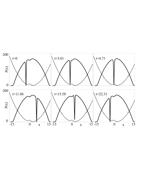
FIG. 1.: Density $|\psi|^{2}$ for a dark soliton oscillating through a static Thomas-Fermi cloud at $\int dx|\psi|^{2}=300$, with potential $V=0.1x(x-2)+1.1\,{\rm sech}^{2}x$ shown in dots. Initially $q=-2.18$. Eqn. (14) thus predicts the time between turning points (where $|\psi|^{2}=p^{2}=0$ at the minimum) to be $T/2=11.5$; the error of about 4% is indeed $\cal{O}(\epsilon)$.

REFERENCES

- [1] M.H. Anderson, J.R. Ensher, M.R. Matthews, C.E. Wieman and E.A. Cornell, Science, 269, 198 (1995); C.C. Bradley, C.A. Sackett, J.J. Tollett and R.G. Hulet, Phys. Rev. Lett. 75, 1687 (1995); K.B. Davis, M.-O. Mewes, M.R. Andrews, N.J. van Druten, D.S. Durfee, D.M. Kurn and W. Ketterle, Phys. Rev. Lett. 75, 3969 (1995).
- [2] W. Ketterle and A. Aspect, private communications.
- [3] W.P. Reinhardt and C.W. Clark, J. Phys. B 30, L785 (1997).
- [4] T.F. Scott, R.J. Ballagh and K. Burnett, J. Phys. B 31, L329-335 (1998).
- [5] R. Dum, J.I. Cirac, M. Lewenstein, and P. Zoller, Phys. Rev. Lett. 80, 2972 (1998).
- [6] E.J. Mueller, P.M. Goldbart and Y. Lyanda-Geller, Phys. Rev. A57, R1505 (1998).
- [7] J. Langer and V. Ambegaokar, Phys. Rev. 164, 498 (1967); D. McCumber and B. Halperin, Phys. Rev. B1, 1054 (1970).
- [8] Y.S. Kivshar and B. Luther-Davies, Phys. Rep. 298, 81 (1998).
- [9] T. Hong, Y.Z. Wang and Y. S. Huo, Phys. Rev. A 58, 3128 (1998).
- [10] S.A. Morgan, R.J. Ballagh and K. Burnett, Phys. Rev. A55, 4338 (1997).
- [11] A.D. Jackson, G.M. Kavoulakis and C.J. Pethick, Phys. Rev. A 58, 2417 (1998).
- [12] A.E. Muryshev, H.B. v. Linden v.d. Heuvell and G.V. Shlyapnikov, cond-mat/9811408; P.O. Fedichev, A.E. Muryshev and G.V. Shlyapnikov, cond-mat/9905062.
- [13] In contrast, the velocity of vortices relative to the ambient superfluid is fixed by the local gradient of the background density: the price of topological stability is a reduced phase space, in which vortex and co-ordinates are canonically conjugate to each other. See B.Y. Rubinstein and L.M. Pismen, Physica D 78, 1 (1994).
- [14] An equation similar to (14) is stated without derivation in Ref. [3], but (when translated into our units) without the factor of . This discrepancy may be seen in a co-ordinate-free way, by noting that in a harmonic trap the GPE as written in [3] implies the same frequency for the collective dipole mode as is given by [3]’s soliton equation of motion. The same equation found in [3] is derived in Ref. [10] by assuming that the soliton does not move relative to the background; this may only be achieved in a locally harmonic trap, in which case the result agrees with our Eqn. (16). Ref. [9] proposes constant, but mentions that oscillation actually occurs instead.
- [15] We use the split-operator technique described in J.A.C. Weideman and B.M. Herbst, SIAM J. Numer. Anal. 23, 485 (1986).
- [16] Th. Busch and J.R. Anglin, in preparation.