Laser probing of atomic Cooper pairs

Abstract

We consider a gas of attractively interacting cold Fermionic atoms which are manipulated by laser light. The laser induces a transition from an internal state with large negative scattering length to one with almost no interactions. The process can be viewed as a tunneling of atomic population between the superconducting and the normal states of the gas. It can be used to detect the BCS-ground state and to measure the superconducting order parameter.

Successful cooling of trapped Fermionic ⁴⁰K atoms down to temperatures where the Fermi degeneracy sets in was reported recently [1, 2]. This breakthrough opens up new opportunities for studying fundamental quantum statistical and many-body physics. A major advantage of Fermionic atoms compared to electrons in condensed matter is the richness of their internal energy structure and the possibility to accurately and efficiently manipulate these energy states by laser light and magnetic fields. Furthermore, atomic gases are dilute and weakly interacting thus offering the ideal tool for developing and experimentally testing theories of many-body quantum physics. A major goal is to observe the predicted [3, 4] BSC-transition for Fermionic atoms – this would compare to the experimental realization of atomic Bose-Einstein condensates [5]. It is still, however, an open question how to observe the BCS-transition, because the value of the superconducting order parameter (gap) is expected to be small and electro-magnetic phenomena such as the Meissner effect do not take place.

We propose a method to detect the existence of the BCS-ground state and to measure the gap using laser light. The main difference in our method compared to the proposals of using off-resonant light scattering [6, 7] is that the light is resonant, that is, population is transferred from one internal state to another. Furthermore, the final state of this process is chosen to have negligible scattering length compared to the initial one: this effectively creates a superconducting – normal state interface across which the atomic population can move. There is a conceptual analogy to electron tunneling from a superconducting metal to a normal one, although the physical systems and their describtions differ in an essential way. Also non-optical phenomena, such as collective and single particle excitations, have been proposed to be used for observing the BCS-transition [8, 9, 10]. The specific feature of our method with respect to other suggested probes, both optical and mechanical (modulating the trap frequency), is the utilization of the superconducting – normal state interface. The advantage is that the normal state population can be initally zero, thus even a small change in it is a significant relative effect. Furthermore, our work offers a basic starting point for describing any phenomenon related to the superconducting–normal interface. For instance, our method can be understood as an outcoupler. With small modifications, one could also describe outcoupling of pairs instead of single atoms which would create an atomic beam with BCS-type statistics.

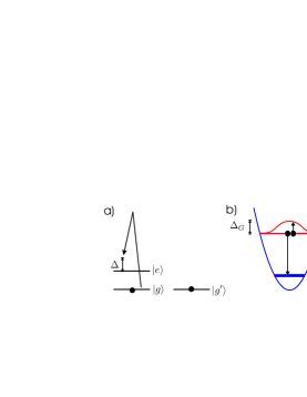
FIG. 1.: Probing of the gap in a gas of attractively interacting cold Fermionic atoms. a) Laser excitation with the coupling $\Omega$ and the detuning $\Delta$ transfers a Cooper paired atom from the internal state $|g\rangle$ to the state $|e\rangle$. b) The other atom in the initial Cooper pair becomes an excitation in the BCS state, therefore the laser has to provide also the additional gap energy $\Delta_{G}$. In this picture the Fermi levels $\mu_{g}$ and $\mu_{e}$ for the internal states have been chosen to be different from each other but they could also equal.

We consider atoms with three internal states available, say $|e\rangle$, $|g\rangle$, and $|g^{\prime}\rangle$. They are chosen so that the interaction between atoms in states $|g\rangle$ and $|g^{\prime}\rangle$ is relatively strong and attractive, and all other interactions are negligible. The laser frequency is chosen to transfer population between $|e\rangle$ and $|g\rangle$, but is not in resonance with any transition which could move population away from the state $|g^{\prime}\rangle$. If there is more or less equal amount of atoms in states $|g\rangle$ and $|g^{\prime}\rangle$ they can form the superconducting BCS ground state; atoms in $|e\rangle$ are in the normal state. For small intensities, the laser-interaction can be treated as a perturbation, the unperturbed states being the normal and the superconducting state. The transfer of atoms from $|g\rangle$ to $|e\rangle$ is then analogous to tunneling of electrons from a normal metal to a superconductor induced by an external voltage, which can be used as a method to probe the gap and the density of states of the superconductor [11]. In our case the tunneling is between two internal states rather than two spatial regions, this resembles the idea of internal Josephson-oscillations in two-component Bose-Einstein condensates [12]. Figure 1 illustrates the basic idea. The observable carrying essential information about the superconducting state is the change in the population of the state $|e\rangle$, we call this the current $I$. Below we calculate the current first in the homogeneous case and then assuming that the atoms are confined in a harmonic trap. Finally will discuss possibilities for experimental realization of the idea, and choosing the states $|e\rangle$, $|g\rangle$, and $|g^{\prime}\rangle$ for ⁶Li.

We define a two-component Fermion field $\psi({\bf x})=(\psi_{e}({\bf x})\quad\psi_{g}({\bf x}))^{T}$, where $\psi_{e}$ and $\psi_{g}$ fulfil standard Fermionic commutation relations. The fields $\psi_{e/g}$ can be expanded using some basis functions (e.g. plane waves or trap wave functions) and corresponding creation and annihilation operators: $\psi_{e/g}({\bf x})=\sum_{j}c_{j}^{e/g}\phi_{j}^{e/g}({\bf x})$. The annihilation and creation operators fulfil $\{{c_{i}^{e}}^{\dagger},c_{j}^{g}\}=0$ and $\{c_{i}^{e/g\dagger},c_{j}^{e/g}\}=\delta_{ij}$. The two components of the field, corresponding to the internal states $|e\rangle$ and $|g\rangle$, are coupled by a laser. This can be either a direct excitation or a Raman process; we denote the atomic energy level difference by $\omega_{a}$ ($\hbar\equiv 1$), the laser frequency $\omega_{L}$ and the wave vector $k_{L}$ – in the case of a Raman process these are effective quantities. In the rotating wave approximation the Hamiltonian reads

$$H = H_{e}+H_{gg^{\prime}}+\frac{\Delta}{2}\int d^{3}x\psi^{\dagger}({\bf x})\sigma_{z}\psi({\bf x})$$ (4)

$$+\int d^{3}x\psi^{\dagger}({\bf x})\left(\begin{array}[]{cc}0&\Omega({\bf x})\\ \Omega^{*}({\bf x})&0\end{array}\right)\psi({\bf x}).$$

Here $\Delta=\omega_{a}-\omega_{L}$ is the (effective) detuning, and $\Omega({\bf x})$ contains the spatial dependence of the laser field multiplied with the (effective) Rabi frequency. The parts $H_{e}$ and $H_{gg^{\prime}}$ contain terms which depend only on $\psi_{e}$ or $\psi_{g}$, $\psi_{g^{\prime}}$, respectively. Possible spatial inhomogeneity, e.g. from the trap potential, is also included in $H_{e}$ and $H_{gg^{\prime}}$.

The observable carrying essential information about the superconducting state is the rate of change in population of the $|e\rangle$ state. We may call it, after the electron tunneling analogy, the current $I(t)=-\langle\dot{N_{e}}\rangle$, where $N_{e}=\int d^{3}x\psi_{e}^{\dagger}({\bf x})\psi_{e}({\bf x})$. The current $I(t)$ is calculated considering the tunneling part of the Hamiltonian, $H_{T}=H-(H_{e}+H_{gg^{\prime}}+\Delta/2(N_{e}-N_{g}))$ as a perturbation; the current $I$ becomes the first order response to the external perturbation caused by the laser. We calculate it both in the homogeneous case and in the case of harmonic confinement. The calculations are done in the grand canonical ensemble, therefore the chemical potentials $\mu_{g}$ and $\mu_{e}$ are introduced. Also the detuning $\Delta$ acts like a difference in chemical potentials, thus it becomes useful to define an effective quantity of the form $\tilde{\Delta}=\mu_{e}-\mu_{g}+\Delta\equiv\Delta\mu+\Delta$. In the derivation we assume finite temperature, but here we only quote the results for $T=0$.

Homogeneous case: The assumption of spatial homogeneity is appropriate when the atoms are confined in a trap potential which changes very little compared to characteristic quantities of the system, such as the coherence length and the size of the Cooper pairs. In the homogeneous case we expand the Fermion fields $\psi_{e/g}$ into plane waves. The Hamiltonian becomes

$$H = H_{e}+H_{gg^{\prime}}+\frac{\Delta}{2}\sum_{k}[{c_{k}^{e}}^{\dagger}c_{k}^{e}-{c_{k}^{g}}^{\dagger}c_{k}^{g}]$$ (6)

$$+\sum_{kl}[T_{kl}{c_{k}^{e}}^{\dagger}c_{l}^{g}+h.c.],$$

where $T_{kl}=\frac{1}{V}\int d^{3}x\Omega({\bf x})e^{i{\bf k}\cdot{\bf x}}e^{-i{\bf l}\cdot{\bf x}}$. We calculate the current $I=-\langle\dot{N_{e}}\rangle=-i\langle[H,N_{e}]\rangle$ treating $H_{T}$ as a perturbation: terms of higher order than $H_{T}^{2}$ are neglected. Because we are interested in the current between the superconducting and normal states, correlations of the form $\langle c_{e}^{\dagger}c_{e}^{\dagger}c_{g}c_{g}\rangle$ (and $h.c.$) are omitted since they correspond to tunneling of pairs (Josephson current). The current can be written

$$I=\int_{-\infty}^{\infty}dt\theta(t)(e^{-i\tilde{\Delta}t}\langle[A^{\dagger}(0),A(t)]\rangle-e^{i\tilde{\Delta}t}\langle[A(0),A^{\dagger}(t)]\rangle)$$ (7)

where $A(t)=\sum_{kl}T_{kl}{c_{k}^{g}}^{\dagger}(t)c_{l}^{e}(t)$, and $c_{l}^{e/g}(t)=e^{iKt}c_{l}^{e/g}e^{-iKt}$ where $K=H-\mu_{e}N_{e}-\mu_{g}N_{g}$. The two terms in the above equation have the form of retarded and advanced Green’s functions. These are evaluated using Matsubara Green’s functions techniques, which leads to $I=\sum_{kl}|T_{kl}|^{2}\int_{-\infty}^{\infty}\frac{d\epsilon}{2\pi}[n_{F}(\epsilon)-n_{F}(\epsilon+\tilde{\Delta})]A_{g}(k,\epsilon+\tilde{\Delta})A_{e}(l,\epsilon),$ where $n_{F}$ are the Fermi distribution functions and $A_{g/e}$ are the spectral functions for the superconducting and normal states. We use the standard expressions $A_{e}(l,\epsilon)=2\pi\delta(\epsilon-\xi_{l})$ and $A_{g}(k,\epsilon+\tilde{\Delta})=2\pi[u_{k}^{2}\delta(\epsilon+\tilde{\Delta}-\omega_{k})+v_{k}^{2}\delta(\epsilon+\tilde{\Delta}+\omega_{k})]$ [11]. Here $\xi_{l}=E_{l}-\mu_{e}$ and $u_{k}$, $v_{k}$ and $\omega_{k}$ are given by the Bogoliubov transformation. Because we are interested in the tunneling out of the superconductor, only the term proportional to $v_{k}^{2}$ is considered. The laser field is chosen to be a running wave, that is $\Omega({\bf x})=\Omega e^{i{\bf k_{L}}\cdot{\bf x}}$. The term $|T_{kl}|^{2}$ now produces a delta-function enforcing momentum conservation. Note that this is very different from the assumption of a constant transfer matrix ($\sum_{kl}|T_{kl}|^{2}\longrightarrow|T|^{2}\sum_{kl}$) made in the standard calculation for tunneling of electrons over a superconductor – normal metal surface [11]. The final result becomes (assuming $T=0$)

$$I=-2\pi\Omega^{2}\rho\theta(-\tilde{\Delta}-\omega_{\tilde{k}-k_{L}}-\Delta\mu)\frac{\omega_{\tilde{k}-k_{L}}-\xi_{\tilde{k}-k_{L}}}{\omega_{\tilde{k}-k_{L}}+\xi_{\tilde{k}-k_{L}}\left[1-\frac{k_{L}}{\tilde{k}}\right]}$$ (8)

where $\tilde{k}$ is given by the following energy conservation condition: $-\tilde{\Delta}+\omega_{\tilde{k}-k_{L}}+\xi_{\tilde{k}-k_{L}}=0$, $\omega_{k}=\sqrt{\xi_{k}^{2}+\Delta_{G}^{2}}$, and $\rho$ is the density of states which appears when the summation over momenta is changed into an integration over energies.

The laser momentum $k_{L}$ can be very small compared to the momentum of the atoms, especially in the case of a Raman process. By setting $k_{L}=0$ the result becomes (choosing $\tilde{\Delta}<0$ i.e. current from $|g\rangle$ to $|e\rangle$)

$$I=-2\pi\Omega^{2}\rho\theta(\tilde{\Delta}^{2}-\Delta_{G}^{2}+2\Delta\mu\tilde{\Delta})\frac{\Delta_{G}^{2}}{\tilde{\Delta}^{2}}.$$ (9)

To understand the results in terms of physics, let us first consider the case of equal chemical potentials $\Delta\mu=0$:

$$I=-2\pi\Omega^{2}\rho\theta(-\Delta-\Delta_{G})\frac{\Delta_{G}^{2}}{\Delta^{2}}.$$ (10)

In order to transfer one atom from the state $|g\rangle$ to $|e\rangle$ the laser has to break a Cooper pair. The minimum energy required for this is the gap energy $\Delta_{G}$, therefore the current does not flow before the laser detuning provides this energy – this is expressed by the step function in (10). As $|\Delta|$ increases further, the current will decrease quadratically. This is because the case $|\Delta|=\Delta_{G}$ corresponds to the transfer of particles with $p=p_{F}$, whereas larger $|\Delta|$ means larger momenta, and there are simply fewer Cooper-pairs away from the Fermi surface. This behaviour is very different from the electron tunneling where the current grows as $\sqrt{(eV)^{2}-\Delta_{G}^{2}}$ [11] (the voltage $eV$ corresponds to the detuning $\Delta$ in our case) because all momentum states are coupled to each other.

When the chemical potentials are not equal the situation is more complicated, but the basic features are the same: i) treshold for the onset of the current given basically by the gap energy, and ii) further decay of the current because the density of the states that can fulfil energy and momentum conservation decreases.

Harmonic confinement: The trap wave functions provide the natural basis of expansion when the atoms are confined in a harmonic trap. We will not, however, do this expansion from the beginning of the calculations but rather derive the current and the corresponding (position dependent) Green’s functions directly for the Fermion fields $\psi_{e/g}$. The current becomes $I=2Im[X_{ret}(-\tilde{\Delta})]$,

$$X_{ret}(-\tilde{\Delta})=\int_{-\infty}^{\infty}\frac{d\epsilon}{2\pi}\int d^{3}x\int d^{3}x^{\prime}\Omega^{*}({\bf x})\Omega({\bf x^{\prime}})$$ (11)

$$[\tilde{A}_{e}({\bf x},{\bf x^{\prime}},\epsilon)G_{adv}^{g}({\bf x^{\prime}},{\bf x},\epsilon+\tilde{\Delta})$$ (12)

$$+G_{ret}^{e}({\bf x},{\bf x^{\prime}},\epsilon-\tilde{\Delta})\tilde{A}_{g}({\bf x^{\prime}},{\bf x},\epsilon)],$$ (13)

and $\tilde{A}_{e/g}$ are defined $\tilde{A}_{e/g}({\bf x},{\bf x^{\prime}},\epsilon)=i(G_{ret}^{e/g}({\bf x},{\bf x^{\prime}},\epsilon)-G_{adv}^{e/g}({\bf x},{\bf x^{\prime}},\epsilon))$. In order to take the imaginary part of the expression (13) we use the following Green’s functions

$$G_{adv}^{g}({\bf x^{\prime}},{\bf x},\epsilon) = \sum_{n}\frac{u_{n}({\bf x^{\prime}})u_{n}^{*}({\bf x})}{\epsilon-\omega_{n}-i\delta}+\frac{v_{n}^{*}({\bf x^{\prime}})v_{n}({\bf x})}{\epsilon+\omega_{n}-i\delta}$$ (14)

$$G_{ret}^{e}({\bf x},{\bf x^{\prime}},\epsilon) = \sum_{n}\frac{\phi_{n}({\bf x})\phi_{n}^{*}({\bf x^{\prime}})}{\epsilon-\xi_{n}+i\delta}.$$ (15)

Here $u_{n}({\bf x})$, $v_{n}({\bf x})$ and $\omega_{n}$ are given by the Bogoliubov–DeGennes equations [13]. We also use the fact that the trap wave functions $\phi_{m}({\bf x})$ are real. The derivation gives

$$I = -2\pi\sum_{n,m}\left|\int d^{3}x\Omega({\bf x})u_{n}({\bf x})\phi_{m}({\bf x})\right|^{2}[n_{F}(\omega_{n})-n_{F}(\xi_{m})]$$ (18)

$$\delta(\xi_{m}+\tilde{\Delta}-\omega_{n})+\left|\int d^{3}x\Omega({\bf x})v_{n}^{*}({\bf x})\phi_{m}({\bf x})\right|^{2}$$

$$[n_{F}(-\omega_{n})-n_{F}(\xi_{m})]\delta(\xi_{m}+\tilde{\Delta}+\omega_{n}).$$

Again, we consider only the term proportional to $v_{n}$, assume zero temperature and use the known form for the trap energy $\xi_{m}=m\Omega_{t}-\mu_{e}$ to obtain the final result

$$I=\frac{2\pi}{\Omega_{t}}\sum_{n}\theta(-\tilde{\Delta}+\omega_{n})\left|\int d^{3}x\Omega({\bf x})v_{n}^{*}({\bf x})\phi_{M}({\bf x})\right|^{2},$$ (19)

where the quantum number $M=(\mu_{e}-\tilde{\Delta}+\omega_{n})/\Omega_{t}$. Although the result is not as transparent as in the homogeneous case, the characteristic treshold behaviour is expressed by the step function. Since the functions inside the absolute square are typically oscillating ones, this term would restrict the values of $n$ in the summation. We have checked that with strong approximations one obtains again the homogeneous case result.

Experimental realization: Typical experimental parameters in the case of ⁶Li are $\Omega_{t}/2\pi\sim 150Hz$ for the trap frequency and $\mu_{g}\sim 100kHz$ for the chemical potential [14]. The order of magnitude of the gap is $\Delta_{G}/\epsilon_{F}\sim 0.1$ (see e.g. [6]). In Figure 2 we show the dependence of the current on the detuning in the homogeneous case, for $\Delta_{G}=0.1\mu_{g}$. The sharp peak given by the result of Eq.(9) will be broadened in an experimental situation. One of the main causes of broadening is that it is difficult to fix the particle number with high accuracy. We have simulated this by assuming that the particle number ($\mu_{g}$) varies from experiment to experiment according to a Gaussian distribution (the width of the Gaussian is used as a measure of the fluctuations), and averaged over the different results. In these calculations we have introduced corresponding Gaussian fluctuations in the gap energy, because it is determined by the particle number. For as large as 10% fluctuations in the gap the peak is still clearly visible although broadened and slightly shifted.

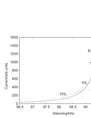
FIG. 2.: The absolute value of the current $I=-\langle\dot{N}_{e}\rangle$ as a function of the laser detuning $\Delta$. The chemical potentials are $\mu_{g}=100kHz$ and $\mu_{e}=0$. The current is calculated assuming 1%, 5%, and 10% fluctuations in the gap energy. Corresponding fluctuations in the particle number ($\mu_{g}$) are taken into account using the exponential dependence between the Fermi energy and the gap energy. The unit of the current is arbitrary. In the case of a normal state, there would be a sharp peak at $\Delta=100=\mu_{g}-\mu_{e}$. Due to the superconducting gap this peak is shifted and its shape modified.

It is possible to prepare the desired initial number of atoms in states $|e\rangle$, $|g\rangle$ and $|g^{\prime}\rangle$ very accurately by applying suitable incoherent laser pulses — this is one of the advantages of atomic Fermi gases compared to condensed matter systems. The number of atoms in the states $|g\rangle$ and $|g^{\prime}\rangle$ should be nearly equal to produce the superconducting state, whereas the number of atoms in state $|e\rangle$ is not critical. In the simplest case the state $|e\rangle$ would be empty in the beginning. The use of our method then requires to know $\mu_{g}$ rather accurately, since it appears in the tunable argument $\tilde{\Delta}=\Delta\mu+\Delta=-\mu_{g}+\Delta$ of the current $I(\tilde{\Delta})$. If this is difficult, it might be better to use an incoherent pulse to prepare initially $\Delta\mu=\mu_{e}-\mu_{g}=0$. In this case the chemical potential dependence disappears from the expressions in the homogeneous case.

Finally, we discuss how to choose the states $|e\rangle$, $|g\rangle$ and $|g^{\prime}\rangle$ for a real atom (for instance ⁶Li). It will probably be difficult to find states in which the atoms do not interact at all. A more likely solution is to choose the states so that the interaction between all of them is weak and repulsive, except between $|g\rangle$ and $|g^{\prime}\rangle$ strong and attractive. Even a weak and attractive interaction instead of weak and repulsive would do, because the gap, critical temperature, and other essential BCS quantities have an exponential dependence on the scattering length, so the effect becomes easily negligible. Particularly ⁶Li seems to offer a variety of interaction strengths between different states. As shown in [15], in a magnetic field of about $B\simeq 0.02T$ the scattering lenght of several low field seeking hyperfine states is as strong as $a_{S}\sim-2000a_{0}$ whereas the scattering length between two high field seeking states is around zero. This is an example of the potential of modifying the scattering lengths by magnetic fields. In this case the trap should be optical in order to confine also the high field seekers. Alternatively, in a magnetic trap atoms in these states (corresponds to the non-interacting state $|e\rangle$ in our calculation) would simply fly out — this could even make the detection of the current easier. The detection of the atoms in the state $|e\rangle$, that is, the measurement of our basic observable $I$, could be done for instance by direct resonance fluorescence, or when a Raman process is used, indirectly from the intensity difference of the two Raman beams.

In conclusion, we have proposed a method to observe the superconducting order parameter (gap) in a gas of cold Fermionic atoms. The idea is based on creating a normal phase – superconductor interface by coupling internal states of different scattering lengths by a laser. The advantage of our scheme is the sensitivity to even small currents of atomic population caused by the laser interaction. Furthermore, our results extend beyond measuring the order parameter: they can be used as a starting point in describing various processes related to the transfer of atoms between two gas components (in superconducting or normal states). If both of the internal states used were strongly interacting, one could perhaps observe Josepson tunneling of pairs from one superconductor to another. With small modifications, our results also describe the functioning of an outcoupler from a superconducting gas of Fermionic atoms.

Acknowledgements We thank H.T.C. Stoof for useful discussions. PT acknowledges the support by the TMR programme of the European Commission (ERBFMBICT983061) and the Academy of Finland (projects 42588 and 47140).

REFERENCES

- [1] B. DeMarco and D.S. Jin, Science 285, 1703 (1999).
- [2] For theoretical work on cold atomic Fermi-gases see e.g. J. Ruostekoski and J. Javanainen, Phys. Rev. Lett. 82, 4741 (1999) and references therein.
- [3] H.T.C. Stoof et al., Phys. Rev. Lett. 76, 10 (1996).
- [4] L. You and M. Marinescu, Phys. Rev. A 60, 2324 (1999).
- [5] For recent reviews, see E.A. Cornell et al., cond-mat/9903109; W. Ketterle et al., cond-mat/9904034.
- [6] F. Weig and W. Zwerger, cond-mat/9908176.
- [7] W. Zhang et al., Phys. Rev. A 60, 504 (1999).
- [8] M.A. Baranov, cond-mat/9801142.
- [9] M.A. Baranov and D.S. Petrov, cond-mat/9901108.
- [10] G.M. Bruun and C.W. Clark, cond-mat/990392.
- [11] G.D. Mahan, Many-Particle Physics (Plenum Press, New York, 1990).
- [12] J. Williams et al., Phys. Rev. A 59, R31 (1999).
- [13] P.G. de Gennes, Superconductivity of Metals and Alloys, (Addison-Wesley Publishing Company, 1989).
- [14] M. Houbiers et al., Phys. Rev. A 56, 4864 (1997).
- [15] M. Houbiers et al., Phys. Rev. A 57, R1497 (1998).