[

Electron momentum distribution in underdoped cuprates

Abstract

We investigate the electron momentum distribution function (EMD) in a weakly doped two-dimensional quantum antiferromagnet (AFM) as described by the $t$-$J$ model. Our analytical results for a single hole in an AFM based on the self-consistent Born approximation (SCBA) indicate an anomalous momentum dependence of EMD showing ’hole pockets’ coexisting with a signature of an emerging large Fermi surface. The position of the incipient Fermi surface and the structure of the EMD is determined by the momentum of the ground state. Our analysis shows that this result remains robust in the presence of next-nearest neighbor hopping terms in the model. Exact diagonalization results for small clusters are with the SCBA reproduced quantitatively.

]

One of the most intriguing questions concerning the superconducting cuprates is the existence and the character of the Fermi surface (FS), in particular in their underdoped regime. This problem has been intensively studied experimentally with the angle-resolved photoemission spectroscopy (ARPES) [1, 2, 3, 4]. There have been also several theoretical investigations of this problem, using the exact diagonalization (ED) of small clusters [5, 6, 7], string calculations [8], slave-boson theory [9] and the high temperature expansion [10]. While a consensus has been reached about the existence of a large Fermi surface in the optimum-doped and overdoped materials, in the interpretation of ARPES experiments for the underdoped cuprates [3] the issue of the debate is (i) why are experiments more consistent with the existence of parts of large FS, i.e., rather Fermi arcs or Fermi patches [4, 11] than with a ’hole pocket’ type small FS, predicted by several theoretical methods based on the existence of AFM long range order in cuprates, (ii) how does a partial FS eventually evolve with doping into a large closed one.

The electron momentum distribution function $n_{\bf k}=\langle\Psi_{{\bf k}_{0}}|\sum_{\sigma}c_{{\bf k},\sigma}^{\dagger}c_{{\bf k},\sigma}|\Psi_{{\bf k}_{0}}\rangle$ is the key quantity for resolving the problem of the Fermi surface. In this paper we study the EMD for $|\Psi_{{\bf k}_{0}}\rangle$ which represents a weakly doped AFM, i.e, it is the ground state (GS) wave function of a planar AFM with one hole and the GS wave vector ${\bf k}_{0}$. In the present work we investigate the low-energy physics of the CuO₂ planes in cuprates within the framework of the standard $t$-$J$ model with nearest-neighbor hopping $t_{ii^{\prime}}\equiv t$ and the AFM exchange $J$. In order to come closer to the realistic situation in cuprates the model is extended with the next-nearest-neighbor hopping $t_{ii^{\prime}}\equiv t^{\prime}$ and the third-neighbor hopping terms $t_{ii^{\prime}}\equiv t^{\prime\prime}$, for $ii^{\prime}$ representing next-nearest-neighbors and third-neighbors, respectively[12] ,

$$H = -\sum_{<ii^{\prime}>\sigma}t_{ii^{\prime}}\bigl{(}{\tilde{c}}_{i,\sigma}^{\dagger}{\tilde{c}}_{i^{\prime},\sigma}+\mbox{H.c.}\bigr{)}+$$ (2)

$$+J\sum_{<ij>}\bigl{[}S_{i}^{z}S_{j}^{z}+\frac{\gamma}{2}(S_{i}^{+}S_{j}^{-}+S_{i}^{-}S_{j}^{+})\bigr{]}.$$

${\tilde{c}}_{i,\sigma}^{\dagger}$ (${\tilde{c}}_{i,\sigma}$) are electron creation (annihilation) operators acting in a space forbidding double occupancy on the same site. The effect of double occupancy [13] on $n_{\bf k}$ is not studied in the present framework of the $t$-$J$ model. $S^{\alpha}_{i}$ are spin operators. For convenience we treat the anisotropy $\gamma$ as a free parameter, with $\gamma=0$ in the Ising limit, and $\gamma\to 1$ in the Heisenberg model. Recent studies of the $t$-$J$ model with $t^{\prime}$, $t^{\prime\prime}$ terms included have shown a very good agreement of the calculated quasiparticle (QP) dispersion with experimental results of ARPES [12] whereby quantitative differences between different Cu compounds have been attributed to different values of $t^{\prime}$ and $t^{\prime\prime}$ [14].

Our analytical approach is based on a spinless fermion – Schwinger boson representation of the $t$-$J$ Hamiltonian [15] and on the SCBA for calculating both the Green’s function [15, 16, 17] and the corresponding wave function [18, 19]. The method is known to be successful in determining spectral and other properties of the QP. In contrast to other methods the SCBA is expected to describe the long-wavelength physics since it is determined by the linear dispersion of spin waves. The short-wavelength properties can be studied with various methods, here we compare the SCBA results with the corresponding ED, as shown further-on.

In the SCBA fermion operators are decoupled into hole and pseudo spin - local boson operators: ${\tilde{c}}_{i,\uparrow}\!=\!h^{\dagger}_{i}$, ${\tilde{c}}_{i,\downarrow}\!=\!h^{\dagger}_{i}S^{+}_{i}\!\sim\!h^{\dagger}_{i}a_{i}$ and ${\tilde{c}}_{i,\downarrow}\!=\!h^{\dagger}_{i}$, ${\tilde{c}}_{i,\uparrow}\!=\!h^{\dagger}_{i}S^{-}_{i}\!\sim\!h^{\dagger}_{i}a_{i}$ for $i$ belonging to $A$- and $B$-sublattice, respectively. The effective Hamiltonian emerges [15, 16, 17, 20]

$${\tilde{H}} = \sum_{\bf k}\epsilon^{0}_{\bf k}h^{\dagger}_{\bf k}h_{\bf k}+\sum_{\bf q}\omega_{\bf q}\alpha^{\dagger}_{\bf q}\alpha_{\bf q}+$$ (4)

$$+N^{-1/2}\sum_{{{\bf k}}{{\bf q}}}(M_{{\bf k}{\bf q}}h_{{{\bf k}}-{{\bf q}}}^{\dagger}h_{{{\bf k}}}\alpha_{{\bf q}}^{\dagger}+{\rm H.c.}),$$

where $h_{\bf k}^{\dagger}$ is the creation operator for a (spinless) hole in a Bloch state with a dispersion $\epsilon^{0}_{\bf k}=4t^{\prime}\cos k_{x}\cos k_{y}+2t^{\prime\prime}(\cos 2k_{x}-\cos 2k_{y})$. The AFM boson operator $\alpha^{\dagger}_{\bf q}$ creates an AFM magnon with the energy $\omega_{\bf q}$, $M_{{\bf k}{\bf q}}$ is the fermion-magnon coupling and $N$ is the number of lattice sites.

We calculate the Green’s function for a hole $G_{\bf k}(\omega)$ within the SCBA [15, 16, 17]. This approximation amounts to the summation of non-crossing diagrams to all orders and the corresponding ground state wave function with momentum ${\bf k}_{0}$ and energy $\epsilon_{{\bf k}_{0}}$ [18, 19] is represented as

$$|\Psi_{{\bf k}_{0}}\rangle = Z^{1/2}_{{\bf k}_{0}}\Bigl{[}h_{{\bf k}}^{\dagger}+N^{-1/2}\sum_{{\bf q}_{1}}M_{{\bf k}_{0}{\bf q}_{1}}G_{\bar{\bf k}_{1}}(\bar{\omega}_{1})h_{\bar{\bf k}_{1}}^{\dagger}\alpha_{{\bf q}_{1}}^{\dagger}+$$ (7)

$$...+N^{-n/2}\!\!\!\sum_{{\bf q}_{1},...,{\bf q}_{n}}\!\!\!M_{{\bf k}{\bf q}_{1}}G_{\bar{\bf k}_{1}}(\bar{\omega}_{1})\,...\,M_{\bar{\bf k}_{n-1}{\bf q}_{n}}\times$$

$$\quad\quad\times\;G_{\bar{\bf k}_{n}}(\bar{\omega}_{n})\;h_{\bar{\bf k}_{n}}^{\dagger}\alpha_{{\bf q}_{1}}^{\dagger}...\,\alpha_{{\bf q}_{n}}^{\dagger}+\,\,\,...\,\,\,\Bigr{]}|0\rangle.$$

Here $\bar{\bf k}_{m}={\bf k}_{0}\!-\!{\bf q}_{1}\!-\!...\!-\!{\bf q}_{m}$, $\bar{\omega}_{m}=\epsilon_{{\bf k}_{0}}\!-\!\omega_{{\bf q}_{1}}\!-\!...\!-\!\omega_{{\bf q}_{m}}$ and $Z_{{\bf k}_{0}}$ is the QP spectral weight. The wave function is properly normalized $\langle\Psi_{{\bf k}_{0}}|\Psi_{{\bf k}_{0}}\rangle=1$ provided the number of magnon terms $n\to\infty$ [19].

The wave function Eq. (7) corresponds to the projected space of the model Eq. (2) and therefore the EMD is $n_{\bf k}=\langle\Psi_{{\bf k}_{0}}|{n_{\bf k}}|\Psi_{{\bf k}_{0}}\rangle=\langle\Psi_{{\bf k}_{0}}|{\tilde{n}_{\bf k}}|\Psi_{{\bf k}_{0}}\rangle$ with the projected electron number operator ${\tilde{n}_{\bf k}}=\sum_{\sigma}{\tilde{c}}_{{\bf k},\sigma}^{\dagger}{\tilde{c}}_{{\bf k},\sigma}$. Consistent with the SCBA approach, we decouple the latter into hole and magnon operators,

$${\tilde{n}_{\bf k}} = \frac{1}{N}{\sum_{ij}}e^{-{\bf k}\cdot({\bf R}_{i}-{\bf R}_{j})}h_{i}h_{j}^{\dagger}\times$$ (9)

$$\times\biggl{(}\eta^{+}_{ij}\bigl{[}1+a_{i}^{\dagger}a_{j}(1-\delta_{ij})\bigr{]}+\eta^{-}_{ij}(a_{i}^{\dagger}+a_{j})\biggr{)},$$

where $\eta^{\pm}_{ij}=(1\pm e^{-{\bf Q}\cdot({\bf R}_{i}-{\bf R}_{j})})/2$ with ${\bf Q}=(\pi,\pi)$. Local $a^{\dagger}_{i}$ are further expressed with proper magnon operators $\alpha^{\dagger}_{\bf q}$. It should be noted that $n_{\bf k}$ should obey the sum rule ${\bar{n}}=\frac{1}{N}\sum_{\bf k}n_{\bf k}=1-c_{\rm h}$ and the constraint $n_{\bf k}\leq 1+c_{\rm h}$, where $c_{\rm h}$ is the concentration of holes[5, 21].

In general the expectation value $n_{\bf k}$ for a single hole has to be calculated numerically and has the following structure

$$n_{\bf k}=1-\frac{1}{2}Z_{{\bf k}_{0}}(\delta_{{\bf k}{\bf k}_{0}}+\delta_{{\bf k}{\bf k}_{0}+{\bf Q}})+{1\over N}\delta n_{\bf k}.$$ (10)

Here the second term proportional to $\delta$-functions corresponds to ’hole pockets’. Note that $\delta n_{\bf k}$, for the case of a single hole fulfills the sum rule $\frac{1}{N}\sum_{\bf k}\delta n_{\bf k}=Z_{{\bf k}_{0}}-1$ and $\delta n_{\bf k}\leq 1$. The introduction of $\delta n_{\bf k}$ is convenient as it allows the comparison of results obtained with different methods and on clusters of different size $N$.

For the case of Ising limit, $\gamma=0$, the Green’s function in the SCBA is independent of ${\bf k}$, $G_{\bf k}(\omega)=G_{0}(\omega)$. Therefore it is possible to express all required matrix elements of $n_{\bf k}$ analytically and to perform a summation of corresponding non-crossing contributions to any order $n$, similar to Ref. [19]. The result for $J/t=0.3$ (as relevant to cuprates) is for some selected directions in the BZ presented in Fig. 1. We have also checked the convergence of $\delta n_{\bf k}$ with the number of magnon lines, $n$. For $J/t\gtrsim 0.3$ we find for all ${\bf k}$ that the contribution of terms $n>3$ amounts to less than few percent. This is in agreement with the convergence of the norm of the wave function, which is even faster [19]. In Fig. 2(a) we present this $\delta n_{\bf k}$ for the whole BZ. Here we note one interesting feature in the Ising limit, i.e., the dip of $\delta n_{\bf k}$ in the center of the BZ at $k\sim 0$ in agreement with Ref. [8].

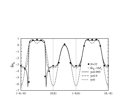
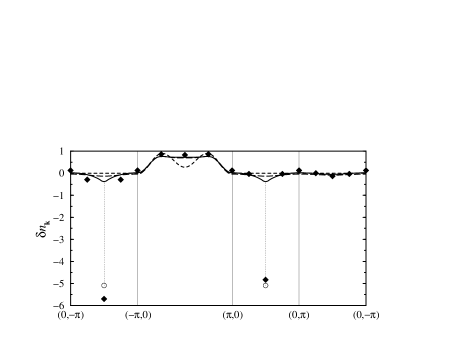
FIG. 1.: $\delta n_{\bf k}$ along selected paths in the BZ for $\gamma=0$, $0.9$, $0.999$. Full diamonds represent ED results $N(n_{\bf k}-1)$ for $N=32$ of Chernyshev et al. [7]. Open circles represent the SCBA result for $\delta n_{{\bf k}_{0}}-\frac{1}{2}NZ_{{\bf k}_{0}}$.

Now we turn to the Heisenberg model, $\gamma\to 1$. Here the important ingredient is the gap-less magnons with linear dispersion and a more complex ground state of the planar AFM. $G_{\bf k}(\omega)$ and $\epsilon_{\bf k}$ become strongly ${\bf k}$-dependent. As a consequence $n_{\bf k}$ is now in general dependent both on ${\bf k}$ and ${\bf k}_{0}$. The ground state is for the $t$-$J$ model fourfold degenerate and we choose ${\bf k}_{0}=(\frac{\pi}{2},\frac{\pi}{2})$. Results should be averaged over all four possible ground state momenta if compared with, e.g., high temperature expansion results [10] or discussed in connection with ARPES data.

Let us first discuss the result in the limit $t/J\to 0$, i.e., for a static hole. In the linearized model, Eq. (4), $M_{\bf kq}=0$. Therefore the hole is not coupled to the AFM ($Z_{{\bf k}_{0}}\equiv 1$) and $\delta n_{\bf k}$ should be zero. However, a straightforward use of Eq. (9) leads also to non-vanishing and momentum dependent $\delta n_{\bf k}=n_{0}({\bf k})$. We attribute this momentum dependence to the improper decomposition of ${\tilde{c}_{i,\sigma}}$ into linearized pseudo spin operators instead of Schwinger bosons obeying the local constraints [15]. In the results for $\delta n_{\bf k}$ presented in this paper (also at finite $J/t$) the contribution $n_{0}({\bf k})$ is not included.

In Fig. 1 we present $\delta n_{\bf k}$ for the $t$-$J$ model with (almost) isotropic Heisenberg exchange, $\gamma=0.999$. Numerical calculations are henceforth performed for $J/t=0.3$ and $N$ corresponding to a $64\times 64$ sites cluster [16]. In evaluating the matrix elements we take into account only terms with up to $n=3$ magnon lines in $|\Psi_{{\bf k}_{0}}\rangle$ [19]. The sum rule of our numerical results for $\delta n_{\bf k}$ is nevertheless fulfilled $\gtrsim 96\%$.

Also included in Fig. 1 are results obtained with ED of the $N=32$ sites cluster[7]. These data are scaled as the quantity $N(n_{\bf k}-1)$ which should be directly compared with the SCBA result $\delta n_{\bf k}$. At momenta ${\bf k}={\bf k}_{0}$, ${\bf k}_{0}+{\bf Q}$, however, one has to take into account contributions from ’hole pocket’ terms proportional to $\delta_{{\bf k}{\bf k}_{0}}$ and with the scaling $\propto N$. Thus ED data should be compared at these points with $\delta n_{{\bf k}_{0}}-\frac{1}{2}NZ_{{\bf k}_{0}}$ calculated from the SCBA. Note also, that the SCBA result for $\gamma=0.9$ (also presented in Fig. 1) represents an intermediate step between the Ising limit and the Heisenberg limit: the dip at the $\Gamma$ point, which is in the Ising limit well pronounced here disappears but the difference for directions ${\bf k}\parallel{\bf k}_{0}$ and ${\bf k}\perp{\bf k}_{0}$ is not yet developed. In Fig. 2(b) we present $\delta n_{\bf k}$ for the Heisenberg limit ($\gamma=0.99)$ in the entire BZ. In comparison with the Ising limit, Fig. 2(a), $\delta n_{\bf k}$ exhibits a very strong momentum dependence around $\pm{\bf k}_{0}$.

The comparison of the SCBA with ED results shows a quantitative agreement at all points in the BZ. However, the SCBA result is symmetric around $\Gamma$ point in the direction ${\bf k}\parallel{\bf k}_{0}$, while small system results show a weak asymmetry for ${\bf k}=\pm{\bf k}_{0}$, respectively. From our analysis of the SCBA results for $N\to\infty$ and long range AFM spin background it follows that $n_{\bf k}$ is in the thermodynamic limit $c_{\rm h}\to 0$ symmetric. The asymmetry is in Ref. [7] attributed to the opening of the gap in the magnon spectrum at ${\bf q}\sim{\bf Q}$ in finite systems. Within the SCBA the asymmetry also appears if the EMD is evaluated with ${\bf k}_{0}$ displaced from $(\frac{\pi}{2},\frac{\pi}{2})$ by a small amount $\delta{\bf k}_{0}$ (not shown here). A common feature of finite clusters is a non-vanishing expectation value of the current operator for the allowed GS wave vector. The GS with vanishing current may be reached by the method of twisted boundary conditions [22], resulting in the GS momentum displaced away from $(\frac{\pi}{2},\frac{\pi}{2})$. The asymmetry of $n_{\bf k}$ found in small clusters can thus be attributed to this displacement and is a finite size effect. In the thermodynamic limit in the system with AFM order the GS momentum would coincide with $(\frac{\pi}{2},\frac{\pi}{2})$ and no asymmetry is expected in $n_{\bf k}$.

To get more insight into the structure of $\delta n_{\bf k}$, we simplify the wave function, Eq. (7), by keeping only the one-magnon contributions. The leading order contribution to $\delta n_{\bf k}$ is

$$\delta n_{\bf k}^{(1)}\!\! = \!-Z_{{\bf k}_{0}}M_{{\bf k}_{0}{\bf q}}G_{{\bf k}_{0}}(\epsilon_{{\bf k}_{0}}\!\!-\!\omega_{\bf q})\bigl{[}2u_{\bf q}\!+\!M_{{\bf k}_{0}{\bf q}}G_{{\bf k}_{0}}(\epsilon_{{\bf k}_{0}}\!\!-\!\omega_{\bf q})\bigr{]}$$ (11)

$$\sim -8Z_{{\bf k}_{0}}^{2}J{{\bf q}\cdot{\bf v}\over\omega^{2}_{\bf q}}(1+Z_{{\bf k}_{0}}{{\bf q}\cdot{\bf v}\over\omega_{\bf q}}),\qquad{q\to 0},$$ (12)

with ${\bf q}={\bf k}-{\bf k}_{0}$ (or ${\bf k}-{\bf k}_{0}-{\bf Q}$) and ${\bf v}=t(\sin k_{0x},\sin k_{0y})$. The momentum dependence of EMD, contained in $\delta n_{\bf k}^{(1)}$, essentially captures well the full numerical solution for the isotropic case, Fig. 2(b), as well as in the Ising limit, Fig. 2(a).

FIG. 2.: $\delta n_{\bf k}$ for (a) the Ising model $\gamma=0$, (b) $\gamma=0.99$ and $t^{\prime}\!=\!t^{\prime\prime}\!=\!0$, and (c) $t$-$t^{\prime}$-$J$ model with $t^{\prime}=0.25t$ and $\gamma=0.99$.

A surprising observation is that the EMD exhibits in the extreme Heisenberg limit for momenta ${\bf k}\sim{\bf k}_{0},{\bf k}_{0}+{\bf Q}$ a discontinuity $\sim Z_{{\bf k}_{0}}N^{1/2}$ and $\delta n_{\bf k}^{(1)}\propto-(1+{\rm sign}\,q_{x})/q_{x}$. These discontinuities are clearly seen in Fig. 1, Fig. 2(b) and are consistent with ED results, Fig. 1. One can interpret this result as an indication of an emerging large Fermi surface at ${\bf k}\sim\pm{\bf k}_{0}$. The discontinuity appears only as points $\pm{\bf k}_{0}$, not lines in the BZ. Note, however, that this result is obtained in the extreme low doping limit, i.e., $c_{\rm h}=1/N$ and it is not straightforward to generalize it to the finite doping regime. In the limit $\gamma\to 1$ this term does not strictly obey the constraint $\delta n_{\bf k}\leq 1$, although due to the symmetry it does not violate the EMD sum rule. The singularity is weak and on introducing a slight anisotropy, e.g. $\gamma\lesssim 0.999$, the constraint is not violated.

In Fig. 3 we present the results for the $t$-$t^{\prime}$-$t^{\prime\prime}$-$J$ model. First we introduce positive next-nearest neighbor hopping matrix elements $t^{\prime}=t/4$, $t^{\prime\prime}=0$, claimed to be appropriate to electron doped systems such as Nd₂Ce cuprates [23]. The GS is now twofold degenerate, with the momenta at corners of the AFM zone, e.g., ${\bf k}_{0}=(\pi,0)$, with an enhanced pole residue $Z_{{\bf k}_{0}}=0.54$. The result is presented in Fig. 2(c) for the entire BZ. The discontinuity in this case disappears due to the symmetry as evident from ${\bf v}=0$ in the leading order approximation, Eq. (12). The effect of negative $t^{\prime}=-t/4$, $t^{\prime\prime}=0$ is relatively weak: the GS momentum remains at ${\bf k}_{0}=(\frac{\pi}{2},\frac{\pi}{2})$, $\delta n_{\bf k}$ at ${\bf k}={\bf Q}$ is lower than the $t^{\prime}=t^{\prime\prime}=0$ result while the discontinuity is smaller, because $Z_{{\bf k}_{0}}=0.25$ here. In Fig. 3 we additionally present results for $N(n_{\bf k}-1)$ obtained from exact diagonalization of a $N=\sqrt{20}\times\sqrt{20}$ cluster. The $t^{\prime}=t^{\prime\prime}=0$ results are in agreement with those of Ref. [7]. All ED results quantitatively confirm the SCBA values. A possible set of parameters appropriate for reproducing the dispersion from experimental ARPES data is $t^{\prime}=-t/4$, $t^{\prime\prime}=t/5$ [12]. Our SCBA result presented in Fig. 3 is qualitatively similar to other $t^{\prime}\leq 0$ results. The main difference is a more pronounced step at ${\bf k}=\pm{\bf k}_{0}$.

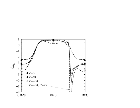
FIG. 3.: $\delta n_{\bf k}$ for different $t^{\prime}$ and $t^{\prime\prime}$. Symbols and lines represent ED for $N=20$ sites and SCBA results, respectively. Full circle and full line denote $t^{\prime}\!=\!t^{\prime\prime}\!=\!0$, full diamonds and long dashed line $t^{\prime}\!=\!t/4$, $t^{\prime\prime}\!=\!0$ and empty diamonds, dot-dashed line $t^{\prime}\!=\!-t/4$, $t^{\prime\prime}\!=\!0$. Short dashed line represents the SCBA result for $t^{\prime}\!=\!-t/4$, $t^{\prime\prime}\!=\!t/5$. In all cases $\gamma=0.999$.

In the present work we considered the electron momentum distribution function in underdoped cuprates. The results of the two methods, the self consistent Born approximation and the exact diagonalization agree quantitatively. Our analysis shows that the presence of next-nearest neighbor terms changes EMD only quantitatively if the ground state is at $(\frac{\pi}{2},\frac{\pi}{2})$ and qualitatively for sufficiently large $t^{\prime\prime}>0$ where the GS momentum is at $(\pi,0)$.

The main observation is however the coexistence of two apparently contradicting Fermi-surface scenarios in EMD of a single hole in an AFM. (i) On one hand, the $\delta$-function contributions in Eq.(5) seem to indicate that at finite doping a delta-function might develop into small Fermi surface, i.e., a hole pocket, provided that AFM long range order persists. (ii) A novel feature is that also $\delta n_{\bf k}$ is singular in a particular way, i.e., it shows a discontinuity at ${\bf k}={\bf k}_{0}$ with a strong asymmetry with respect to ${\bf k}_{0}$. It is therefore more consistent with infinitesimally short arc (point) of an emerging large FS. For finite doping the discontinuity could possibly extend into such a finite arc (not closed) FS. Note that as long-range AFM order is destroyed by doping, ’hole-pocket’ contributions should disappear while the singularity in $\delta n_{\bf k}$ could persist.

Making contact with ARPES experiments we should note that ARPES measures the imaginary part of the electron Green’s function. We must note that using these experiments in underdoped cuprates $n_{\bf k}$ can be only qualitatively discussed since the latter is extracted only from rather restricted frequency window below the chemical potential. Nevertheless our results are not consistent with a small hole-pocket FS (at least only a part of presumable closed FS is visible), but rather with partially developed arcs resulting in FS which is just a set of disconnected segments at low temperature collapsing to the point [4]. The SCBA results for singular $\delta n_{\bf k}$ seem to allow for such a scenario. It should also be stressed that the SCBA approach is based on the AFM long-range order, still we do not expect that finite but longer-range AFM correlations would entirely change our conclusions.

REFERENCES

- [1] Z.-X. Shen and D. S. Dessau, Phys. Rep. 253, 1 (1995).
- [2] B. O. Wells et al., Phys. Rev. Lett. 74, 964 (1995).
- [3] D. S. Marshall et al., Phys. Rev. Lett. 76, 4841 (1996).
- [4] M. R. Norman et al., Nature 392, 157 (1998).
- [5] W. Stephan and P. Horsch, Phys. Rev. Lett. 66, 2258 (1991).
- [6] R. Eder and Y. Ohta, Phys. Rev. B 57, R5590 (1998).
- [7] A. L. Chernyshev, P. W. Leung and R. J. Gooding, Phys. Rev. B 58, 13594 (1998).
- [8] R. Eder, Phys. Rev. B, 44, R12609 (1991).
- [9] X.-G. Wen and P. A. Lee, Phys. Rev. Lett. 76, 503 (1996).
- [10] W. O. Putikka, M. U. Luchini, and R. R. P. Singh, J. Phys. Chem. Solids 59, 1858 (1998); Phys. Rev. Lett. 81, 2966 (1998).
- [11] N. Furukawa, T. M. Rice, and M. Salmhofer, Phys. Rev. Lett., 81, 3195 (1998).
- [12] B. Kyung and R. A. Ferrell, Phys. Rev. B 54, 10125 (1996); O. P. Sushkov, G. A. Sawatzky, R. Eder, and H. Eskes, Phys. Rev. B 56, 11769 (1997); T. Xiang and J. M. Wheatley, Phys. Rev. B 54, R12653 (1996).
- [13] H. Eskes and R. Eder, Phys. Rev. B 54, 14226 (1996); F. Lema and A. A. Aligia, Phys. Rev. B 55, 14092 (1997).
- [14] L. F. Feiner, J. H. Jefferson, and R. Raimondi, Phys. Rev. Lett. 76, 4939 (1996).
- [15] S. Schmitt-Rink, C. M. Varma, and A. E. Ruckenstein, Phys. Rev. Lett. 60, 2793 (1988); C. L. Kane, P. A. Lee, and N. Read, Phys. Rev. B 39, 6880 (1989).
- [16] A. Ramšak and P. Prelovšek, Phys. Rev. B 42, 10415 (1990).
- [17] G. Martínez and P. Horsch, Phys. Rev. B 44, 317 (1991).
- [18] G. F. Reiter, Phys. Rev. B 49, 1536 (1994).
- [19] A. Ramšak and P. Horsch, Phys. Rev. B 48, 10559 (1993); ibid. 57, 4308 (1998).
- [20] J. Bała, A. M. Oleś, and J. Zaanen, Phys. Rev. B 52, 4597 (1995).
- [21] J. Jaklič and P. Prelovšek, Phys. Rev. B 55, R7307 (1997).
- [22] X. Zotos, P. Prelovšek and I. Sega, Phys. Rev. B 42, 8445 (1990).
- [23] T. Tohyama and S. Maekawa, J. Phys. Soc. Jpn. 59, 1760 (1990).