To be published in Solid State Commun. 113, No. 12, p. 683 (2000).
Two-dimensional charged electron-hole complexes in magnetic fields:
Keeping magnetic translations preserved

Abstract

Eigenstates of two-dimensional charged electron-hole complexes in magnetic fields are considered. The operator formalism that allows one to partially separate the center-of-mass motion from internal degrees of freedom is presented. The scheme using magnetic translations is developed for calculating in strong magnetic fields the eigenspectra of negatively charged excitons $X^{-}$, a bound state of two electrons and one hole.

1 Introduction

Identification [1] of charged excitons in magneto-optical spectra of quasi-two-dimensional (quasi-2D) systems has induced much interest in the behavior of these three-particle electron-hole ($e$–$h$) complexes. The negatively, $X^{-}$, and positively, $X^{+}$, charged excitons are the bound states of two electrons and one hole ($2e$–$h$) and two holes and one electron ($2h$–$e$), respectively. In magnetic fields $B$, in addition to the spin-singlet, higher-lying triplet states of $X^{-}$ and $X^{+}$ have been observed [1]. Theoretically, free charged excitons have been studied in strictly 2D systems in the limit of high [2] and low [3] magnetic fields and in quasi-2D systems at high magnetic fields [4, 5]. For one-component electron systems in magnetic fields, the center-of-mass motion separates from internal degrees of freedom. The well-known Kohn theorem [6], which states that the electron cyclotron resonance is not shifted or broadened by electron-electron interactions, is based on this fact. For $e$–$h$ systems such a complete separation is not possible in magnetic fields. Nonetheless, any charged interacting system in a uniform $B$ possesses an exact dynamical symmetry — magnetic translations ([7, 8] and references therein). It has been shown recently [9] that due to this symmetry, magneto-optical transitions of charged $e$–$h$ complexes are governed by an exact selection rule, which leads to some rather unexpected spectroscopic consequences for charged excitons in $B$. In this work, using an operator formalism, we construct a basis compatible with the exact dynamical symmetries — rotations about the $B$-axis and magnetic translations. Physically, this is equivalent to a partial separation of the center-of-mass motion from internal degrees of freedom in $B$ [7, 8]. We demonstrate that this basis can be used for high-accuracy and rapidly convergent calculations of bound $X^{-}$ states in strong magnetic fields. Our results can also be relevant for atomic ions with not too large mass ratios in ultrastrong magnetic fields [8].

2 Basis compatible with magnetic translations

We consider a strictly 2D system containing two electrons and one hole in a perpendicular magnetic field ${\bf B}=(0,0,B)$ described by the Hamiltonian

$$H = H_{0}+H_{\rm ee}+H_{\rm eh}\,,$$ (1)

$$H_{0} = \sum_{i=1,2}\frac{\hat{\mbox{\boldmath$\pi$}}_{ei}^{2}}{2m_{e}}+\frac{\hat{\mbox{\boldmath$\pi$}}_{h}^{2}}{2m_{h}}\,,$$ (2)

$$H_{\rm ee} = \frac{e^{2}}{\epsilon|{\bf r}_{1}-{\bf r}_{2}|}\quad,\quad H_{\rm eh}=-\sum_{i=1,2}\frac{e^{2}}{\epsilon|{\bf r}_{i}-{\bf r}_{h}|}\,,$$ (3)

where $\hat{\mbox{\boldmath$\pi$}}_{j}=-i\hbar\mbox{\boldmath$\nabla$}_{j}-\frac{e_{j}}{c}{\bf A}({\bf r}_{j})$ are kinematic momentum operators. We will use the symmetric gauge ${\bf A}=\frac{1}{2}{\bf B}\times{\bf r}$. The exact eigenstates can be characterized by the total angular momentum projection $M_{z}$, an eigenvalue of $\hat{L}_{z}=\sum_{j}({\bf r}_{j}\times-i\hbar\mbox{\boldmath$\nabla$}_{j})_{z}$, by the total spin of two electrons $S_{e}=0$ (singlet states) or $S_{e}=1$ (triplet states), and the spin state of the hole $S_{h}$. The latter simply factors out and will be disregarded. Performing an orthogonal transformation of the coordinates $\{{\bf r}_{1},{\bf r}_{2},{\bf r}_{h}\}\rightarrow\{{\bf r},{\bf R},{\bf r}_{h}\}$, where ${\bf r}=({\bf r}_{1}-{\bf r}_{2})/\sqrt{2}$ is the electron relative and ${\bf R}=({\bf r}_{1}+{\bf r}_{2})/\sqrt{2}$ center-of-mass coordinates, the complete orthonormal basis with a fixed value of $M_{z}$ can be constructed [10] (see also [11]) as an expansion in Landau levels (LL’s)

$$\phi^{(e)}_{n_{1}m_{1}}({\bf r})\,\phi^{(e)}_{n_{2}m_{2}}({\bf R})\,\phi^{(h)}_{n_{h}m_{h}}({\bf r}_{h})\,.$$ (4)

Here $\phi^{(e)}_{nm}({\bf r})=\phi^{(h)*}_{nm}({\bf r})$ are the $e$- and $h$- single-particle factored wave functions in $B$; $n$ is the LL quantum number and $m$ is the oscillator quantum number (see, e.g., [7, 8]). For, e.g., zero LL’s

$$\phi^{(e)*}_{0m}({\bf r})=\phi^{(h)}_{0m}({\bf r})=\frac{1}{(2\pi m!\ell_{B}^{2})^{1/2}}\left(\frac{z}{\sqrt{2}\ell_{B}}\right)^{m}\exp\left(-\frac{r^{2}}{4\ell_{B}^{2}}\right)\,,$$ (5)

where $z=x+iy$ is the 2D complex coordinate and $\ell_{B}=(\hbar c/eB)^{1/2}$. The factored wave functions are constructed with the help of the oscillator Bose ladder operators: For electrons (the charge $-e<0$)

$$\phi^{(e)}_{nm}({\bf r})=\frac{1}{\sqrt{n!m!}}\langle{\bf r}|(A^{{\dagger}}_{e})^{n}(B^{{\dagger}}_{e})^{m}|0\rangle\,,$$ (6)

here the intra-LL operators $B^{{\dagger}}_{e}({\bf r}_{j})=-i\sqrt{c/2\hbar Be}\,\hat{K}_{j-}$, where $\hat{K}_{j\pm}=\hat{K}_{jx}\pm i\hat{K}_{jy}$ and $\hat{\bf K}_{j}=\hat{\mbox{\boldmath$\pi$}}_{j}-\frac{e_{j}}{c}{\bf r}_{j}\times{\bf B}$ (see, e.g., [7, 8]). The electron inter-LL operators are $A^{{\dagger}}_{e}({\bf r}_{j})=-i\sqrt{c/2\hbar Be}\,\hat{\pi}_{j+}$, where $\hat{\pi}_{j\pm}=\hat{\pi}_{jx}\pm i\hat{\pi}_{jy}$. The operators commute as $[A_{e},A^{{\dagger}}_{e}]=1$, $[B_{e},B^{{\dagger}}_{e}]=1$, and $[A_{e},B^{{\dagger}}_{e}]=[A_{e},B_{e}]=0$. The analogous intra-LL and inter-LL operators for the hole (the charge $e>0$) are, respectively, $B^{{\dagger}}_{h}({\bf r}_{h})=-i\sqrt{c/2\hbar Be}\,\hat{K}_{h+}$ and $A^{{\dagger}}_{h}({\bf r}_{h})=-i\sqrt{c/2\hbar Be}\,\hat{\pi}_{h-}$. These can be considered as linear functions of spatial coordinates and derivatives and have the form

$$A^{{\dagger}}_{e}({\bf r})=B^{{\dagger}}_{h}({\bf r}) = \frac{1}{\sqrt{2}}\left(\frac{z}{2\ell_{B}}-2\ell_{B}\frac{\partial}{\partial z^{\ast}}\right)\,,$$ (7)

$$B^{{\dagger}}_{e}({\bf r})=A^{{\dagger}}_{h}({\bf r}) = \frac{1}{\sqrt{2}}\left(\frac{z^{\ast}}{2\ell_{B}}-2\ell_{B}\frac{\partial}{\partial z}\right)\,.$$ (8)

Single-particle angular momentum projection operators $\hat{L}_{ze}=A^{{\dagger}}_{e}A_{e}-B^{{\dagger}}_{e}B_{e}$ and $\hat{L}_{zh}=B^{{\dagger}}_{h}B_{h}-A^{{\dagger}}_{h}A_{h}$, so that $m_{ze}=-m_{zh}=n-m$. The basis (4) includes therefore different three-particle $2e$–$h$ states such that $M_{z}=n_{1}+n_{2}-m_{1}-m_{2}-n_{h}+m_{h}$ is fixed. Permutational symmetry of identical particles requires that for electrons in the spin-singlet $S_{e}=0$ (triplet $S_{e}=1$) state the relative motion angular momentum $n_{1}-m_{1}$ should be even (odd). The basis (4) proved to be effective in strong $B$ for studying impurity-bound states of $e$–$h$ complexes [10], collective excitations — magnetoplasmons and spin-waves [12], and effects of lateral confinement in quantum dots in $B$ [13, 14]. The equivalent LL expansion (using the coordinates $\{{\bf r}_{1},{\bf r}_{2},{\bf r}_{h}\}$) has been exploited [4, 5] for studying free charged excitons in $B$. However, for translationally invariant systems the basis (4) is not compatible with the magnetic translations.

Indeed, the Hamiltonian (1) commutes with the operator of the magnetic translations $\hat{\bf K}=\sum_{j}\hat{\bf K}_{j}$ [7, 8]. Noting that $[\hat{K}_{x},\hat{K}_{y}]=-i\frac{\hbar B}{c}Q$, where the total charge $Q\equiv\sum_{j}e_{j}=-e$ for the $X^{-}$, one obtains the lowering and raising Bose ladder operators for the whole system [7, 8, 9]

$$\hat{k}_{\pm}=\pm\frac{i}{\sqrt{2}}(\hat{k}_{x}\pm i\hat{k}_{y})\quad,\quad[\hat{k}_{+},\hat{k}_{-}]=-\frac{Q}{|Q|}=1\,,$$ (9)

here $\hat{{\bf k}}=\sqrt{c/\hbar B|Q|}\,\hat{\bf K}$. Therefore, $\hat{{\bf k}}^{2}=\hat{k}_{+}\hat{k}_{-}+\hat{k}_{-}\hat{k}_{+}$ has the discrete oscillator eigenvalues $2k+1$, $k=0,1,\ldots$. These can be used, together with $M_{z}$, for labelling of exact charged eigenstates of (1). Due to the non-commutativity of $\hat{K}_{x}$ and $\hat{K}_{y}$, there is the macroscopic Landau degeneracy in $k$. Note now that $\hat{{\bf k}}^{2}=\left(\sum_{j}\hat{{\bf k}}_{j}\right)^{2}=\sum_{j}\hat{{\bf k}}^{2}_{j}+\sum_{i\neq j}\hat{{\bf k}}_{i}\cdot\hat{{\bf k}}_{j}$ is not diagonal in the basis (4) due to the cross terms $\sum_{i\neq j}\hat{{\bf k}}_{i}\cdot\hat{{\bf k}}_{j}$.

In order to make the basis (4) compatible with the magnetic translations, a canonical transformation diagonalizing $\hat{{\bf k}}^{2}$ should be performed. We deal formally with a set of coupled harmonic oscillators. Note then that

$$\hat{k}_{-}=B_{e}^{{\dagger}}({\bf r}_{1})+B_{e}^{{\dagger}}({\bf r}_{2})-B_{h}({\bf r}_{h})=\sqrt{2}\,B_{e}^{{\dagger}}({\bf R})-B_{h}({\bf r}_{h})$$ (10)

and define

$$\tilde{B}_{e}^{{\dagger}}({\bf R})=uB^{{\dagger}}_{e}({\bf R})-vB_{h}({\bf r}_{h})\quad,\quad\tilde{B}_{e}({\bf R})=uB_{e}({\bf R})-vB^{{\dagger}}_{h}({\bf r}_{h})\,,$$ (11)

where $u=\sqrt{2}$, $v=1$. It is this pair of Bose ladder operators in which $\hat{{\bf k}}^{2}$ is diagonal: $\hat{{\bf k}}^{2}=2\tilde{B}_{e}^{{\dagger}}\tilde{B}_{e}+1$. Equation (11) is in fact a Bogoliubov canonical transformation $\tilde{B}_{e}^{{\dagger}}=SB_{e}^{{\dagger}}S^{{\dagger}}$ generated by the unitary operator (see, e.g., [15, 16])

$$S=\exp\{\Theta[B_{e}({\bf R})B_{h}({\bf r}_{h})-B^{{\dagger}}_{h}({\bf r}_{h})B^{{\dagger}}_{e}({\bf R})]\}$$ (12)

with $u={\rm ch}\Theta=\sqrt{2}$, $v={\rm sh}\Theta=1$. The second pair of linearly independent transformed operators $\tilde{B}_{h}^{{\dagger}}({\bf r}_{h})=SB^{{\dagger}}_{h}({\bf r}_{h})S^{{\dagger}}$ and $\tilde{B}_{h}({\bf r}_{h})=SB_{h}({\bf r}_{h})S^{{\dagger}}$ are

$$\tilde{B}_{h}^{{\dagger}}({\bf r}_{h})=uB^{{\dagger}}_{h}({\bf r}_{h})-vB_{e}({\bf R})\quad,\quad\tilde{B}_{h}({\bf r}_{h})=uB_{h}({\bf r}_{h})-vB^{{\dagger}}_{e}({\bf R})\,.$$ (13)

The complete orthogonal basis compatible with both axial and translational symmetries therefore is

$$A_{e}^{{\dagger}}({\bf r})^{n_{1}}A_{e}^{{\dagger}}({\bf R})^{n_{2}}A_{h}^{{\dagger}}({\bf r}_{h})^{n_{h}}\tilde{B}_{e}^{{\dagger}}({\bf R})^{k}B_{e}^{{\dagger}}({\bf r})^{m}\tilde{B}_{h}^{{\dagger}}({\bf r}_{h})^{l}|\tilde{0}\rangle\,.$$ (14)

In (14) the oscillator quantum number is fixed and equals $k$ while $M_{z}=-k-m+l+n_{1}+n_{2}-n_{h}$ and $n_{1}-m$ is even (odd) for $S_{e}=0$ ($S_{e}=1$). The Hamiltonian (1) is block-diagonal in the quantum numbers $k,M_{z},S_{e}$. Moreover, due to the Landau degeneracy in $k$, it is sufficient to consider the $k=0$ states only. This effectively removes one degree of freedom and corresponds to a partial separation of the center-of-mass motion from internal degrees of freedom for a charged $e$–$h$ system in a magnetic field (cf. [7, 8]).

In (14) the new vacuum $|\tilde{0}\rangle=S|0\rangle$ has been introduced. Disentangling the operators in the exponent of $S$ (see, e.g., [15, 16]), one obtains

$$S = \exp\left(-{\rm th}\Theta\,B^{{\dagger}}_{h}B^{{\dagger}}_{e}\right)$$

$$\times\exp\left(-\ln({\rm ch}\Theta)[B^{{\dagger}}_{e}B_{e}+B^{{\dagger}}_{h}B_{h}+1]\right)\exp\left({\rm th}\Theta\,B_{e}B_{h}\right)\,,$$

so that

$$|\tilde{0}\rangle=S|0\rangle=\frac{1}{{\rm ch}\Theta}\exp\left(-{\rm th}\Theta\,B^{{\dagger}}_{h}({\bf r}_{h})B^{{\dagger}}_{e}({\bf R})\right)|0\rangle\,.$$ (16)

For a charged system of $N_{e}$ electrons and $N_{h}$ holes (with, e.g., $N_{e}>N_{h}$), a transformation analogous to (11)–(13) can also be performed. It should involve the intra-LL $e$- and $h$- center-of-mass operators $B^{{\dagger}}_{e}({\bf R}_{e})$ and $B_{h}({\bf R}_{h})$ with ${\rm th}\Theta=\sqrt{N_{h}/N_{e}}$; here ${\bf R}_{e}=\sum_{i=1}^{N_{e}}{\bf r}_{ei}/\sqrt{N_{e}}$ and ${\bf R}_{h}=\sum_{j=1}^{N_{h}}{\bf r}_{hj}/\sqrt{N_{h}}$.

3 $X^{-}$ states in lowest Landau levels

We now demonstrate how the developed formalism works. We will consider the limit of high magnetic fields [2, 5, 9]

$$\hbar\omega_{\rm ce}\,,\,\hbar\omega_{\rm ch}\,,\,|\hbar\omega_{\rm ce}-\hbar\omega_{\rm ch}|\gg E_{0}=\sqrt{\frac{\pi}{2}}\,\frac{e^{2}}{\epsilon l_{B}}\,,$$ (17)

when mixing between different LL’s can be neglected. $E_{0}$ is the characteristic energy of the Coulomb interactions in strong $B$, $\hbar\omega_{\rm ce(h)}=\hbar eB/m_{\rm e(h)}c$. Charged magnetoexcitons can then be labeled by the total electron LL number $n_{e}=n_{1}+n_{2}$ and by the hole LL number $n_{h}$. Indeed, when (17) is fulfilled, the states having different quantum numbers $n_{e}n_{h}$ and $n^{\prime}_{e}n^{\prime}_{h}$ are only weakly $\sim E_{0}/|(n^{\prime}_{e}-n_{e})\hbar\omega_{\rm ce}+(n^{\prime}_{h}-n_{h})\hbar\omega_{\rm ch}|$ mixed by the Coulomb interactions [11].

We focus on the states in zero LL’s [$n_{1}=n_{2}=n_{h}=0$ in (14)]. The operators (11), (13) have a simple representation in the new coordinates $\mbox{\boldmath$\rho$}_{1}=\sqrt{2}\,{\bf R}-{\bf r}_{h}$ and $\mbox{\boldmath$\rho$}_{2}=\sqrt{2}\,{\bf r}_{h}-{\bf R}$: $\tilde{B}_{e}^{{\dagger}}({\bf R})=B_{e}^{{\dagger}}(\mbox{\boldmath$\rho$}_{1})$ and $\tilde{B}_{h}^{{\dagger}}({\bf r}_{h})=B_{h}^{{\dagger}}(\mbox{\boldmath$\rho$}_{2})$. The complete infinite orthonormal basis in zero LL’s with fixed $k=0$ and arbitrary $M_{z}=l-m$ takes the form

$$\frac{1}{(m!l!)^{1/2}}B_{e}^{{\dagger}}({\bf r})^{m}B_{h}^{{\dagger}}(\mbox{\boldmath$\rho$}_{2})^{l}|\tilde{0}\rangle\equiv|m\,l\rangle\,$$ (18)

with odd $m=2p+1$ (even $m=2p$), $p=0,1,\ldots$ in the electron triplet $S_{e}=1$ (singlet $S_{e}=0$) states. The Coulomb interactions in the new variables are

$$H_{\rm ee}=\frac{e^{2}}{\sqrt{2}\epsilon r}\quad,\quad H_{\rm eh}=-\frac{\sqrt{2}e^{2}}{\epsilon|\mbox{\boldmath$\rho$}_{2}-{\bf r}|}-\frac{\sqrt{2}e^{2}}{\epsilon|\mbox{\boldmath$\rho$}_{2}+{\bf r}|}\,.$$ (19)

The matrix elements of the $e$–$e$ interaction are diagonal in the basis (18):

$$\langle m_{2}l_{2}|H_{\rm ee}|m_{1}l_{1}\rangle=\delta_{m_{1},m_{2}}\delta_{l_{1},l_{2}}\frac{V_{0,m_{1}}}{\sqrt{2}}\quad,\quad V_{0,m}=\frac{(2m-1)!!}{2^{m}m!}\,E_{0}\,,$$ (20)

where $V_{0,m}$ is the interaction of the electron with a fixed negative charge $-e$ in zero LL (e.g., [10]). Due to the permutational symmetry, the two terms in $H_{\rm eh}$ give the same contributions; calculations, however, are not so straightforward as (20). This is connected with the fact that the coordinate transformation $\{{\bf r},{\bf R},{\bf r}_{h}\}\rightarrow\{{\bf r},\mbox{\boldmath$\rho$}_{1},\mbox{\boldmath$\rho$}_{2}\}$ is not orthogonal. As a result, the coordinate representation of the new vacuum is not factored in $\mbox{\boldmath$\rho$}_{1}$ and $\mbox{\boldmath$\rho$}_{2}$:

$$\langle{\bf r}\mbox{\boldmath$\rho$}_{1}\mbox{\boldmath$\rho$}_{2}|\tilde{0}\rangle=\frac{1}{\sqrt{2}\,(2\pi\ell_{B}^{2})^{3/2}}\exp\left(-\frac{r^{2}+\rho_{1}^{2}+\rho_{2}^{2}+\sqrt{2}Z_{1}Z_{2}^{\ast}}{4\ell_{B}^{2}}\right)\,,$$ (21)

here $Z_{j}=\rho_{jx}+i\rho_{jy}$, $j=1,2$. Therefore, when acting on the vacuum $|\tilde{0}\rangle$, the operator $B_{h}^{{\dagger}}(\mbox{\boldmath$\rho$}_{2})=\tilde{B}_{h}^{{\dagger}}({\bf r}_{h})$ gives a combination $(Z_{2}+\frac{1}{\sqrt{2}}Z_{1})/\sqrt{2}\ell_{B}=z_{h}/2\ell_{B}$. To eliminate the coordinate $\mbox{\boldmath$\rho$}_{1}$, we perform the shift $\mbox{\boldmath$\rho$}_{1}\rightarrow\tilde{\mbox{\boldmath$\rho$}}=\mbox{\boldmath$\rho$}_{1}+\frac{1}{\sqrt{2}}\mbox{\boldmath$\rho$}_{2}=\frac{1}{\sqrt{2}}{\bf R}$ and obtain

$$\langle m_{2}l_{2}|H_{\rm eh}|m_{1}l_{1}\rangle = \int\!\frac{d^{2}{\rho}_{2}}{2\cdot 2\pi\ell_{B}^{2}\sqrt{2^{l_{1}+l_{2}}l_{1}!l_{2}!}}\exp\left(-\frac{{\rho}_{2}^{2}}{4\ell_{B}^{2}}\right)$$

$$\times\int\!d^{2}r\,\phi^{(e)*}_{0m_{2}}({\bf r})\frac{-2\sqrt{2}e^{2}}{\epsilon|\mbox{\boldmath$\rho$}_{2}-{\bf r}|}\phi^{(e)}_{0m_{1}}({\bf r})\int\!\frac{d^{2}\tilde{\rho}}{2\pi\ell_{B}^{2}}\exp\left(-\frac{\tilde{\rho}^{2}}{2\ell_{B}^{2}}\right)$$

$$\times\left(\frac{\tilde{Z}^{\ast}}{\sqrt{2}\ell_{B}}+\frac{Z_{2}^{\ast}}{2\ell_{B}}\right)^{l_{2}}\left(\frac{\tilde{Z}}{\sqrt{2}\ell_{B}}+\frac{Z_{2}}{2\ell_{B}}\right)^{l_{1}}\sim\delta_{l_{1}-m_{1},l_{2}-m_{2}}\,.$$

Integrating out the variable $\tilde{\mbox{\boldmath$\rho$}}$, we reduce the problem to an effective two-particle $e$–$h$ problem in zero LL’s (cf. [10]). The peculiarity of the situation is that the effective particles are characterized by different magnetic lengths. The matrix elements (3) can be presented in the form ($m_{1}=m$, $m_{2}=m+s$, $l_{1}=l$, $l_{2}=l+s$)

$$\langle m\!+\!s\,l\!+\!s|H_{\rm eh}|m\,l\rangle=(-2\sqrt{2})2^{-l-\frac{s}{2}}\sum_{k=0}^{l}\left(C_{l}^{k}C_{l+s}^{k+s}\right)^{\frac{1}{2}}U^{(\alpha=2)}_{km}(s)\,,$$ (23)

where $C_{n}^{m}$ are binomial coefficients and the matrix elements of the Coulomb interparticle interactions in zero LL’s have been introduced:

$$\int\!d^{2}r_{1} \int\!d^{2}r_{2}\,\phi_{0m_{2}}^{(e)*}\left({\bf r}_{1}\right)\phi_{0k_{2}}^{(h)*}\left({\bf r}_{2}/\sqrt{\alpha}\right)\frac{e^{2}}{|{\bf r}_{1}-{\bf r}_{2}|}\phi_{0k_{1}}^{(h)}\left({\bf r}_{2}/\sqrt{\alpha}\right)\phi_{0m_{1}}^{(e)}\left({\bf r}_{1}\right)=$$

$$= \delta_{k_{1}-m_{1},k_{2}-m_{2}}U^{(\alpha)}_{{\rm min}(k_{1},k_{2}),{\rm min}(m_{1},m_{2})}(|m_{1}-m_{2}|)$$ (24)

The matrix elements (3) can be found analytically for arbitrary $\alpha$:

$$U^{(\alpha)}_{mn}(s) = E_{0}\frac{\alpha^{\frac{s}{2}}\left[m!(m+s)!n!(n+s)!\right]^{-\frac{1}{2}}}{(1+\alpha)^{s+\frac{1}{2}}\,2^{m+n+s}}\sum_{k=0}^{m}\,\sum_{l=0}^{n}\,C_{m}^{k}\,C_{n}^{l}$$

$$\times\frac{\alpha^{l}}{(1+\alpha)^{k+l}}\,[2(k+l+s)-1]!!\,[2(m-k)-1]!!\,[2(n-l)-1]!!\,.$$

Equations (20), (23), and (3) determine the secular equation of the infinite order that should be solved to obtain the three-particle $2e$–$h$ states in zero LL’s. A truncation of the basis should naturally be performed. An important property of the developed basis (14) [and (18)] is that such a truncation does not break the translational invariance. On the contrary, a truncation of the basis (4), as performed in [4, 5] (see also [2]), leads to spurious mixing of different $k$-states and violates the exact magneto-optical selection rule [9] — the conservation of the oscillator quantum number $k$.

Table 1: Singlet $X^{-}_{sn_{e}n_{h}}$ and triplet $X^{-}_{tn_{e}n_{h}}$ charged magnetoexcitons in Landau levels $n_{e}n_{h}$

	$M_{z}$	Interaction energy ($E_{0}$)	Binding energy ($E_{0}$)
$X^{-}_{t00}$	-1†	-1.04345	0.04345
$X^{-}_{s01}$	-3‡	-0.78056	0.20690
$X^{-}_{t01}$	-4‡	-0.75776	0.18410
$X^{-}_{t10}$	1†	-1.08596	0.08596

^† the only bound states in the given LL’s $n_{e}n_{h}$.
^‡ the ground states among many other bound states with the same $n_{e}n_{h}$.

The developed approach also provides an effective computational tool: First, we have been able to remove one degree of freedom in the three-particle problem, so that configurational space is substantially reduced (cf. [5]). As a result, with finite-size calculations it is even possible to reproduce with a reasonable accuracy the three-particle continuum — a neutral magnetoexciton plus a scattered electron [9]. Second, for bound $X^{-}$ states lying outside the continua we have extremely rapid convergence within each LL. This is associated with the exponential decay of the off-diagonal matrix elements (23). Consider, e.g., the $k=0$ triplet $X^{-}_{tn_{e}=0n_{h}=0}$ state in zero LL’s with $M_{z}=-1$. The asymptotic behavior of the relevant off-diagonal Coulomb $e$–$h$ matrix elements is

$$\langle 2s\!+\!1\,2s|H_{\rm eh}|1\,0\rangle=-\frac{2\sqrt{2}}{2^{s}}U^{(\alpha=2)}_{01}(2s)\simeq-\sqrt{\frac{32}{27\pi}}\left(\frac{1}{9}\right)^{s}E_{0}\>,\>s\gg 1\,.$$ (26)

Also, even the 1$\times$1 matrix Hamiltonian in the basis (18) $\langle 1\,0|H_{\rm ee}+H_{\rm eh}|1\,0\rangle=-1.0073E_{0}$ ensures the $X^{-}$ binding: it gives a positive binding energy $0.0073E_{0}$; this is relative to the ground state energy $-E_{0}$ of the neutral $X_{n_{e}=0n_{h}=0}$ magnetoexciton in zero LL’s. As a result, the $X^{-}_{t00}$ binding energy can be calculated with virtually unlimited accuracy and equals $0.043452E_{0}$; this value is compatible with [2, 5]. Not accounting for the Landau degeneracy in $k$, the $X^{-}_{t00}$ state with $M_{z}=-1$ is the only low-lying bound $X^{-}$ state in zero LL’s: there are no other bound triplet or singlet states [2, 5, 9].

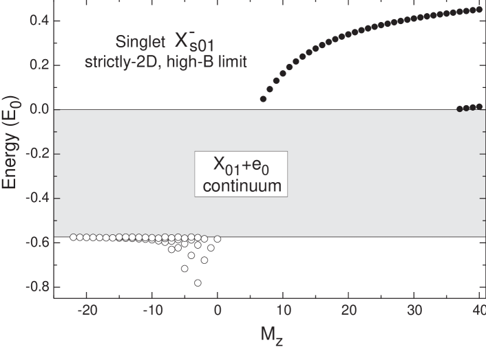
Figure 1: Bound and scattering three-particle $2e$–$h$ singlet $S_{e}=0$ states in the ($n_{e}n_{h}$)=(01) LL’s. Note that only the $k=0$ states are shown. The energy is given relative to the energy of free LL’s $\frac{1}{2}\hbar\omega_{\rm ce}+\frac{3}{2}\hbar\omega_{\rm ch}$, in units of $E_{0}=\sqrt{\pi/2}\,e^{2}/\epsilon l_{B}$. Open circles correspond to low-lying $X^{-}_{s01}$ states. Filled circles correspond to excited states originating from bound internal motion of two electrons in 2D in high magnetic fields. The shaded area shows the continuum corresponding to the neutral magnetoexciton $X_{01}$ plus a scattered electron in the $n_{e}=0$ LL; the lower continuum edge lies at an energy $-0.5737E_{0}$.

Similar considerations apply to the $X^{-}$ states in higher LL’s. Some of the results for the $X^{-}$ ground states are presented in Table 1. There is only one bound $X^{-}$ state in the first electron LL (the basis (14) includes the states with $n_{1}=1$, $n_{2}=0$, $n_{h}=0$ and $n_{1}=0$, $n_{2}=1$, $n_{h}=0$). This state is the triplet $X^{-}_{t10}$ with $M_{z}=1$, whose binding energy is almost twice that of the $X^{-}_{t00}$ state in zero LL’s [9]. This resembles a stronger binding of the triplet $D^{-}$ state (two electrons bound by a donor ion) in the first electron LL [11] and has the same physical origin. The $X^{-}_{t10}$ binding energy is counted from the lowest possible unbound state in the same LL’s, which is the neutral magnetoexciton $X_{n_{e}=0n_{h}=0}$ with the second electron in the scattering state in the $n_{e}=1$ LL. As calculations show, there are many bound $X^{-}$ states in the next hole LL [$n_{1}=n_{2}=0$, $n_{h}=1$ in (14)] — both triplets $X^{-}_{t01}$ and singlets $X^{-}_{s01}$ (see Fig. 1). These are lying below the ground state of the neutral magnetoexciton $X_{n_{e}=0n_{h}=1}$; the latter has the energy $-0.57366E_{0}$. Due to this small binding energy of the neutral $X_{n_{e}=0n_{h}=1}$ magnetoexciton (comparatively to the $X_{n_{e}=0n_{h}=0}$ magnetoexciton), the triplet $X^{-}_{t01}$ and singlet $X^{-}_{s01}$ ground states have rather large binding energies (Table 1). In all LL’s, there are also higher-lying bound three-particle $2e$–$h$ states [9] originating from the internal bound motion of 2D electrons in strong magnetic fields. These states appear in the spectrum at relatively large positive values of the total $M_{z}$, that correspond to the hole being at large distances from the electrons (cf. with the similar states in the $D^{-}$ problem [11]).

4 Summary

In conclusion, we have developed a formalism that allows one to preserve the exact symmetry — magnetic translations — when performing the Landau level expansion for charged electron-hole complexes in magnetic fields. This is achieved by using the Bogoliubov canonical transformation mixing the center-of-mass motions of the electron and hole subsystems. The effectiveness of the scheme has been demonstrated for high-accuracy and rapidly convergent calculations of two-dimensional charged excitons $X^{-}$ in magnetic fields. This can be useful for studying the eigenspectra of charged excitons in quasi-two-dimensional quantum wells at strong and intermediate magnetic fields.

References

• [*] E-mail: dzyub@mandala.th.physik.uni-frankfurt.de
• [1] See, e.g., G. Finkelstein, H. Shtrikman, and I. Bar-Joseph, Phys. Rev. Lett. 74 (1995) 976; A. J. Shields, M. Pepper, M. Y. Simmons, and D. A. Ritchie, Phys. Rev. B 52 (1995) 7841; M. Kozhevnikov, E. Cohen, Arza Ron, H. Shtrikman, and L. N. Pfeiffer, Phys. Rev. B 56 (1997) 2044; H. Okamura, D. Heiman, M. Sundaram, and A. C. Gossard, Phys. Rev. B 58 (1998) R15 985; M. Hayne, C. L. Jones, R. Bogaerts, C. Riva, A. Usher, F. M. Peeters, F. Herlach, V. V. Moshchalkov, and M. Henini, Phys. Rev. B 59 (1999) 2927; S. Glasberg, G. Finkelstein, H. Shtrikman, and I. Bar-Joseph, Phys. Rev. B 59 (1999) R10 425 and references therein.
• [2] J. J. Palacios, D. Yoshioka, and A. H. MacDonald, Phys. Rev. B 54 (1996) R2296.
• [3] B. Stebe, A. Ainane, and F. Dujardin, J. Phys.: Cond. Matter 8 (1996) 5383.
• [4] J. R. Chapman, N. F. Johnson, and V. N. Nicopoulos, Phys. Rev. B 55 (1997) R10 221.
• [5] D. M. Whittaker and A. J. Shields, Phys. Rev. B 56 (1997) 15 185.
• [6] W. Kohn, Phys. Rev. 123 (1961) 1242.
• [7] J. E. Avron, I. W. Herbst, and B. Simon, Ann. Phys. (N.Y.) 114 (1978) 431.
• [8] B. R. Johnson, J. O. Hirschfelder, and K. H. Yang, Rev. Mod. Phys. 55 (1983) 109.
• [9] A. B. Dzyubenko and A. Yu. Sivachenko, Pis’ma ZhÉTF 70 (1999) 504 [JETP Lett. 70 (1999) 514]; cond-mat/9902086.
• [10] A. B. Dzyubenko, Phys. Lett. A 173 (1993) 311.
• [11] A. B. Dzyubenko, Phys. Lett. A 165 (1992) 357; A. B. Dzyubenko and A. Yu. Sivachenko, Phys. Rev. B 48 (1993) 14 690.
• [12] A. B. Dzyubenko and Yu. E. Lozovik, ZhÉTF 104 (1993) 3416 [JETP 77 (1993) 617].
• [13] A. B. Dzyubenko and A. Yu. Sivachenko, J. Phys. IV (Paris) 3 (1993) 381; cond-mat/9908406, to be published in Physica E.
• [14] A. Wójs and P. Hawrylak, Phys. Rev. B 51 (1995) 10 880.
• [15] D. A. Kirzhnits, Field Theoretical Methods in Many-Body Systems, Pergamon Press, Oxford, 1967, p. 372.
• [16] M. Wegner, Unitary Transformations in Solid State Physics, North-Holland, Amsterdam, 1986, Chap. 1, 2.