Electronic Structure of Carbon Nanotube Ropes

Abstract

We present a tight binding theory to analyze the motion of electrons between carbon nanotubes bundled into a carbon nanotube rope. The theory is developed starting from a description of the propagating Bloch waves on ideal tubes, and the effects of intertube motion are treated perturbatively in this basis. Expressions for the interwall tunneling amplitudes between states on neighboring tubes are derived which show the dependence on chiral angles and intratube crystal momenta. We find that conservation of crystal momentum along the tube direction suppresses interwall coherence in a carbon nanorope containing tubes with random chiralities. Numerical calculations are presented which indicate that electronic states in a rope are localized in the transverse direction with a coherence length corresponding to a tube diameter.

I Introduction

A carbon nanotube is a cylindrical tubule formed by wrapping a graphene sheet. Single wall carbon nanotubes (SWNTs) can be synthesized in structures $1$ nm in diameter and microns long [1]. There has been particular interest in the electronic properties of SWNTs which are predicted to exist in both conducting and semiconducting forms [2]. Remarkably, it is possible to probe this behavior experimentally by contacting individual tubes with lithographically patterned electrodes or by tunneling spectroscopy on single tubes [3]. However, most methods for synthesizing carbon nanotubes do not produce isolated tubes; instead the tubes self assemble to form a hierarchy of more complex structures. At the molecular scale tubes pack together to form bundles or “ropes” which can contain 10-200 tubes. X-ray diffraction reveals that a bundle contains tubes close packed in a triangular lattice [1], and measurements of the lattice constant and tube form factor led initially to the suggestion that these ropes contain primarily (10,10) nanotubes, a species predicted to be metallic [2]. Subsequent work has demonstrated that the ropes likely contain a distribution of tube diameters and chiralities [4]. On larger scales the ropes bend and entangle, so that the macroscopic morphology of a carbon nanotube sample is that of an entangled mat. Carbon nanotubes are also formed in various thick multiwalled species which exhibit their own unique electronic behavior [5].

The electronic properties of isolated SWNTs are controlled by the tube’s wrapping vector, curvature and torsion [6]. However, in ropes and in multiwalled tubes the interactions between graphene surfaces is expected to play a major role. This is the case even for crystalline graphite in the Bernal structure. Although an isolated graphene sheet is a zero gap semiconductor, the small residual interactions between neighboring graphene sheets with the ordered $A$-$B$ stacking sequence lead to a small overlap of bands near the Fermi energy and eventually to conducting behavior [7]. Graphite is an ordered three dimensional crystal for which weak intersurface interactions are sufficient to establish quantum coherence for electronic states on neighboring sheets. Thus the electrons can delocalize both parallel to the graphene sheet and perpendicular to it.

Recognizing this, several groups have attempted to estimate the energy scale for similar effects in nanotube ropes [8]. Here the situation is much more delicate, since the structure of a (10,10) nanotube does not permit perfect registry between neighboring tubes when they are packed into a triangular lattice. Nevertheless, it is possible to construct a nanotube crystal, a hypothesized ordered structure in which each (10,10) tube adopts the same orientation, and to study its electronic properties with conventional band theoretic methods [8]. Theoretical studies on nanotube ropes show that intertube interactions in a nanotube crystal lead to a mixing of forward and backward propagating electronic states near the Fermi energy. The level repulsion between these branches leads to suppression or “pseudogap” in the electronic density of states, on an energy scale estimated to be a few tenths of an electron volt. It should be noted that these effects are qualitatively different from those found in graphite where intersurface interactions lead to band overlap and thus an enhancement of the Fermi level density of states.

It has not yet been possible to extend these ideas to carbon nanotube ropes which contain a mixture of tubes with various diameters and chiralities. A direct calculation of the electronic structure for such a rope, which we define as “compositionally disordered,” is quite complicated since the system has no translational symmetry either along the rope axis or perpendicular to it.

In this paper we develop a tight binding theory for the coupling between tubes. In the absence of intertube coupling the electronic states on an isolated tube are essentially the Bloch waves of the graphene sheet wrapped onto the surface of a cylinder and indexed by a two dimensional crystal momentum k. The essence of our theory is to develop the effects of intertube interactions ${\rm t}({\bf k}_{1},{\bf k}_{2})$ perturbatively. We find that the effects of intertube interactions in a disordered rope are quite different from what one obtains for a crystalline rope. In fact, we find that compositional disorder introduces an important energy barrier to inter-tube hopping within a rope so that intertube coherence is strongly suppressed. We are led to conclude that eigenstates in a compositionally disordered rope are strongly localized on individual tubes, though they can extend over large distances along the tube direction. Numerical results illustrating this effect will be presented in this paper. We believe this physics underlies the experimental observation that charge transport at low temperature occurs by hopping conduction in nanotube ropes and mats.

In section II we develop the tunneling model for describing the tight binding coupling between neighboring tubes in a rope. In this section we derive an analytic expression giving the tunneling amplitude ${\rm t({\bf k}_{1},{\bf k}_{2})}$ between Bloch states on neighboring tubes indexed by momenta ${\rm{\bf k}_{1}}$ and ${\rm{\bf k}_{2}}$. In Section III we apply the method to study the electronic structure of a rope crystal, and show that the model reproduces well the results of more complete band theoretic calculations on this ordered system. In Section IV we then extend the method to study the low energy electronic structure in a compositionally disordered rope and analyze the effects of intertube interactions perturbatively. We will also present direct numerical calculations on a compositionally disordered rope which probe the transverse localization of the electronic states. A brief discussion of the relation of these results to experimental data is given in Section V.

II Tunneling Model

In this section we derive an effective tight binding model which describes the coupling between the low energy electronic states on neighboring tubes. This coupling depends on the chirality and orientation of the tubes. Our starting point is a microscopic tight binding model which describes the coupling of the carbon $\pi$ orbitals both within a tube and between tubes,

$${\cal H}={\cal H}_{0}+{\cal H}_{T}.$$ (1)

${\cal H}_{0}$ is a nearest neighbor tight binding model describing uncoupled tubes,

$${\cal H}_{0}=-\sum_{a}\sum_{<ij>}t_{\pi}c_{ai}^{\dagger}c_{aj},$$ (2)

where the index $a$ labels the tubes and $<ij>$ is a sum over nearest neighbor atoms on each tube. Tunneling between tubes is also represented by

$${\cal H}_{T}=\sum_{<ab>}\sum_{ij}t_{ai,bj}c_{ai}^{\dagger}c_{bj}+{\rm H.c.}.$$ (3)

In the following we will assume that $t_{ai,bj}=t_{{\bf r}_{ai},{\bf r}_{bj}}$ depends on the positions and relative orientations of the $\pi$ orbitals on the $i$ and $j$ atoms.

The eigenstates of ${\cal H}_{0}$ are plane waves localized in an individual tube. Due to the translational symmetry of an individual tube the eigenstates may be indexed by a tube index $a$ and a two dimensional momentum ${\bf k}$. Of course the periodic boundary conditions imposed by wrapping the graphene sheet into a cylinder will give a constraint on the possible values of ${\bf k}$. In the following, we wish to express the Hamiltonian in terms of this plane wave basis. We will focus on eigenstates with low energy, which have ${\bf k}$ near one of the corners of the graphite Brillouin zone.

A Plane Wave Basis

It is useful to express the eigenstates of the individual tubes in a basis of plane wave states localized on either the $A$ or $B$ sublattice. Let us first focus on a single tube. The eigenstates may be described by considering a two dimensional graphene sheet with periodic boundary conditions. We will find it useful to consider two coordinate systems for the two dimensional graphene sheet. As shown in Fig. 1, the $x$ and $y$ axes are oriented with respect to the armchair and zig zag axes of the graphene sheet. The $u$ and $v$ axes, on the other hand are oriented with respect to the tube, with $u$ pointing down the tube and $v$ pointing around the circumference. For armchair tubes these axes coincide, and in general the angle between the axes is equal to the chiral angle of the tube.

Suppressing the tube index, for the moment, we let

$$c_{i}={1\over\sqrt{N}}\sum_{\bf k}e^{i{\bf k}\cdot{\bf r}_{i}}c_{\eta(i){\bf k}},$$ (4)

where $\eta$ specifies the $A$ or $B$ sublattice and $N$ is the number of graphite unit cells on the tube. In this basis, the Hamiltonian for an isolated tube may be written

$${\cal H}_{0}=-t_{\pi}\sum_{k}\gamma_{\bf k}c_{A{\bf k}}^{\dagger}c_{B{\bf k}}+{\rm H.c.},$$ (5)

where

$$\gamma_{\bf k}=\sum_{j=1}^{3}e^{i{\bf k}\cdot{\bf d}_{j}}.$$ (6)

Here ${\bf d}_{j}$ are the three nearest neighbor vectors connecting the $A$ and $B$ sublattice indicated in Fig. 1. At low energy we may focus on the points ${\bf k}=\alpha{\bf K}_{\ell}+{\bf q}$, where $\alpha=\pm 1$, ${\bf K}_{\ell}$ are at the corners of the Brillouin zone shown in Fig. 2, and $\ell=-1,0,1$. In the $u-v$ system, the ${\bf K}_{\ell}$ vectors can be written as

$$\alpha{\bf K}_{\ell}=\alpha K_{0}(\cos\omega_{\ell},\sin\omega_{\ell}),$$ (7)

where

$$\omega_{\ell}={2\pi\over 3}\ell+\theta$$ (8)

is the angle that the $\ell^{\mbox{th}}$ Fermi vector makes with the $u$ axis.

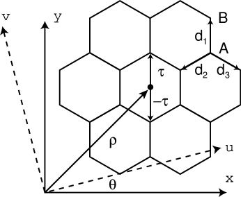
FIG. 1.: A graphene sheet. The $x$ and $y$ axes are oriented with respect to the armchair and zigzag axes, while the $u$ and $v$ axes point in the directions of along and around the tube respectively. The vectors ${\bf d}_{i}$ are the three nearest neighbor vectors connecting the $A$ and $B$ sublattices and ${\bf\rho}$ is the vector point to the center of a hexagon. $\theta$ is the chiral angle.

We will now focus on the point ${\bf K}_{0}$. For small ${\bf q}$, $\gamma_{\alpha{\bf K}_{0}+{\bf q}}=-(\sqrt{3}a/2)(\alpha q_{x}-iq_{y})$. Introducing a spinor $\psi_{\eta\alpha{\bf q}}=c_{\eta\alpha{\bf K}_{0}+{\bf q}}$ the Hamiltonian may then be written,

$${\cal H}_{0}=v\psi_{\alpha{\bf q}}^{\dagger}(\alpha q_{x}\sigma_{x}+q_{y}\sigma_{y})\psi_{\alpha{\bf q}},$$ (9)

where $v=\sqrt{3}t_{\pi}a/2$ and the $\eta$ indices are suppressed.

The tunneling Hamiltonian may similarly be expressed in this plane wave basis. Using (2.4) the term in (2.3) for the bond connecting tubes $a$ and $b$ is

$${1\over N}\sum_{{\bf r}_{a}{\bf r}_{b}}\sum_{{\bf k}_{a}{\bf k}_{b}}t_{{\bf r}_{a}{\bf r}_{b}}e^{i({\bf k}_{b}\cdot{\bf r}_{b}-{\bf k}_{a}\cdot{\bf r}_{a})}c_{a\eta_{a}{\bf k}_{a}}^{\dagger}c_{b\eta_{b}{\bf k}_{b}},$$ (10)

where $\eta_{a,b}$ label the sublattice of the lattice site ${\bf r}_{a,b}$.

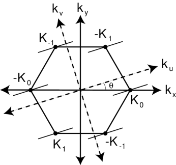
FIG. 2.: Brillouin zone of a graphene sheet. ${\bf K}_{\ell}$, $\ell=-1,0,1$ label the three equivalent Fermi points and $\theta$ is the chiral angle of the tube formed by wrapping the sheet in the $v$ direction.

The sums over lattice sites may be evaluated by introducing a Fourier transform of the tunneling matrix element. As detailed in Appendix A, we may write

$${\cal H}_{T}=\sum_{{\bf G}_{a}{\bf G}_{b}}\sum_{\eta_{a}\eta_{b}}e^{i{\bf G}_{a}\cdot(\rho_{a}+\eta_{a}\tau_{a})-{\bf G}_{b}\cdot(\rho_{b}+\eta_{b}\tau_{b})}t_{{\bf k}_{a}+{\bf G}_{a}{\bf k}_{b}+{\bf G}_{b}}c_{\eta_{a}{\bf k}_{a}}^{\dagger}c_{\eta_{b}{\bf k}_{b}},$$ (11)

where

$$t_{{\bf k}_{a},{\bf k}_{b}}={1\over{NA_{\rm cell}^{2}}}\int d^{2}r_{a}d^{2}r_{b}t({\bf r}_{a},{\bf r}_{b})e^{-i{\bf k}_{a}\cdot{\bf r}_{a}+i{\bf k}_{b}\cdot{\bf r}_{b}},$$ (12)

and $G$ is a reciprocal lattice vector.

We now specialize to eigenstates in the vicinity of the Fermi points, ${\bf k}=\alpha{\bf K}_{0}+{\bf q}$. We may express the sum over the $G$’s as a sum over equivalent ${\bf K}$ points which are related to ${\bf K}_{0}$ by a reciprocal lattice vector. In the following we will see that this sum is dominated by the ${\bf K}_{0}$, ${\bf K}_{1}$ and ${\bf K}_{-1}$, which lie in the “first star” in reciprocal space. Since ${\bf K}_{0}\cdot{\bf\tau}=0$, the sum becomes

$${\cal H}_{T}=\sum_{\alpha_{a}\eta_{a}\alpha_{b}\eta_{b}{\bf q}_{a}{\bf q}_{b}}T(\alpha_{a}\eta_{a}{\bf q}_{a}|\alpha_{b}\eta_{b}{\bf q}_{b})\psi_{a\alpha_{a}\eta_{a}{\bf q}_{a}}^{\dagger}\psi_{b\alpha_{b}\eta_{b}{\bf q}_{b}},$$ (13)

with

$$T(\alpha_{a}\eta_{a}{\bf q}_{a}|\alpha_{b}\eta_{b}{\bf q}_{b})=\sum_{\ell_{a}\ell_{b}=-1}^{1}e^{i\alpha_{a}{\bf K}_{a\ell_{a}}\cdot(\rho_{a}+\eta_{a}\tau_{a})-i\alpha_{b}{\bf K}_{b\ell_{b}}\cdot(\rho_{b}+\eta_{b}\tau_{b})}t_{\alpha_{a}{\bf K}_{a\ell_{a}}+{\bf q}_{a},\alpha_{b}{\bf K}_{b\ell_{b}}+{\bf q}_{b}}.$$ (14)

We shall also find it useful to express the tunneling Hamiltonian in a basis in which the bare Hamiltonian describing the tubes is diagonal. This is accomplished by performing a rotation in the sublattice index space to make (2.9) diagonal. Specifically, for a tube with chiral angle $\theta$, the eigenstates will have momentum ${\bf k}=\alpha{\bf K}_{0}+{\bf q}$, with $(q_{x},q_{y})=q(\cos\theta,\sin\theta)$. Equation (2.9) is then

$${\cal H}_{0}=v\psi^{\dagger}_{\alpha q}\alpha q(e^{-i\alpha\theta}\sigma^{+}+e^{i\alpha\theta}\sigma^{-})\psi_{\alpha q}.$$ (15)

Using the transformation $\psi_{\alpha q}=U(\alpha,\theta)\psi^{\prime}_{\alpha q}$, with

$$U(\alpha,\theta)=e^{-i{1\over 2}\alpha\theta\sigma^{z}}e^{-i{\pi\over 4}\alpha\sigma^{y}},$$ (16)

the Hamiltonian becomes

$${\cal H}_{0}=vq(\psi^{\prime\dagger}_{\alpha qR}\psi^{\prime}_{\alpha qR}-\psi^{\prime\dagger}_{\alpha qL}\psi^{\prime}_{\alpha qL}).$$ (17)

In the $(R,L)$ basis, the tunneling matrix has the form

$$T^{\prime}(\alpha_{a}\eta_{a}^{\prime}{\bf q}_{a}|\alpha_{b}\eta_{b}^{\prime}{\bf q}_{b})=U^{\dagger}(\alpha_{a},\theta_{a})_{\eta_{a}^{\prime}\eta_{a}}T(\alpha_{a}\eta_{a}{\bf q}_{a}|\alpha_{b}\eta_{b}{\bf q}_{b})U(\alpha_{b},\theta_{b})_{\eta_{b}\eta_{b}^{\prime}},$$ (18)

which may be written as

$$T^{\prime}(\alpha_{a}\eta_{a}^{\prime}{\bf q}_{a}|\alpha_{b}\eta_{b}^{\prime}{\bf q}_{b})=\sum_{\ell_{a}\ell_{b}=-1}^{1}e^{i\alpha_{a}{\bf K}_{a\ell_{a}}\cdot\rho_{a}-i\alpha_{b}{\bf K}_{b\ell_{b}}\cdot\rho_{b}}t_{\alpha_{a}{\bf K}_{a\ell_{a}}+{\bf q}_{a},\alpha_{b}{\bf K}_{b\ell_{b}}+{\bf q}_{b}}M_{\eta_{a}^{\prime}\eta_{b}^{\prime}},$$ (19)

where

$$M={1\over 2}\left[\begin{array}[]{*2c}f_{\alpha_{a}}^{\ell_{a}}f_{\alpha_{b}}^{\ell_{b}\ast}&f_{\alpha_{a}}^{\ell_{a}}f_{-\alpha_{b}}^{\ell_{b}\ast}\\ f_{-\alpha_{a}}^{\ell_{a}}f_{\alpha_{b}}^{\ell_{b}\ast}&f_{-\alpha_{a}}^{\ell_{a}}f_{-\alpha_{b}}^{\ell_{b}\ast}\end{array}\right],$$ (20)

$$f_{\alpha}^{\ell}=e^{i\phi_{\ell}}+\alpha e^{-i\phi_{\ell}},$$ (21)

and

$$\phi_{\ell}={1\over 2}(2\pi-\omega_{\ell}).$$ (22)

B Tunneling Matrix Elements

For simplicity, we suppose that the matrix elements $t_{ij}$ for tunneling between atoms on different tubes depend only on the distance between the atoms and are of the form,

$$t_{ij}=t_{0}e^{-d_{ij}/a_{0}},$$ (23)

where $d_{ij}$ is the distance between atoms $i$ and $j$.

It is useful to introduce two dimensional coordinates which are oriented relative to the tube’s axis. Let us define a two dimensional vector ${\bf r}=(u,v)$, where $u$ is the distance down the tube axis, and $v$ is the distance around the tube measured from the “contact line” as shown in Fig. 3.

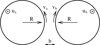
FIG. 3.: cross section of two parallel tubes of radius $R$, and with a separation $b$.

Suppose the two tubes have a separation $b$ as shown in Fig. 3. Then, the distance is given by

$$d({\bf r}_{a},{\bf r}_{b})^{2}= (u_{a}-u_{b})^{2}+(R\sin{v_{a}\over R}-R\sin{v_{b}\over R})^{2}$$ (24)

$$+(b+2R-R\cos{v_{a}\over R}-R\cos{v_{b}\over R})^{2}.$$ (25)

Since the range of the tunneling interaction $a_{0}$ is of order $.5$Å, while $R\approx 7$Åand $b\approx$ 3.4Å, it is useful to expand (2.24) for $u$,$v\ll b$,$R$,

$$d({\bf r}_{a},{\bf r}_{b})=b+{|{\bf r}_{a}-{\bf r}_{b}|^{2}\over{2b}}+{v_{a}^{2}+v_{b}^{2}\over{2R}}.$$ (26)

It follows that the tunneling matrix element has a Gaussian dependence on ${\bf r}_{a}$ and ${\bf r}_{b}$,

$$t({\bf r}_{a},{\bf r}_{b})=t_{0}e^{-b/a_{0}}e^{-{1\over 2}[{|{\bf r}_{a}-{\bf r}_{b}|^{2}\over{ba_{0}}}+{v_{a}^{2}+v_{b}^{2}\over{Ra_{0}}}]}.$$ (27)

We may now use (2.26) to evaluate the Fourier transform of the matrix elements. The Gaussian form allows this to be done simply. Using the fact that the total area of the graphene sheet is given by $NA_{\rm cell}=2\pi RL$, we find

$$t_{{\bf k}_{a}{\bf k}_{b}}={2\pi ba_{0}\over{A_{\rm cell}}}t_{0}e^{-b/a_{0}}e^{-{ba_{0}\over 4}(|{\bf k}_{a}|^{2}+|{\bf k}_{b}|^{2})}\sqrt{a_{0}\over{4\pi R}}e^{-{Ra_{0}\over 4}(k_{av}-k_{bv})^{2}}\delta_{k_{au}k_{bu}}.$$ (28)

We now use (2.27) to evaluate the low energy tunneling matrix elements. Due to the exponential dependence on $|{\bf k}_{a}|^{2}$ the sum on ${\bf K}_{a}$ in (2.11) will be dominated by three terms ${\bf K}_{ai}$ in the “first star” in which $|{\bf K}|=K_{0}=4\pi/(3a)$. Specifically, estimating the parameters $a=2.5$ Å, $b=3.4$ Å and $a_{0}=0.5$ Å, the exponent of the last term is approximately $8\pi^{2}ba_{0}/9a^{2}\approx 2.4$. Thus the next star at $\sqrt{3}K_{0}$ will be suppressed by a factor of $\exp(-2(2.4))=0.01$, justifying the first star approximation. For ${\bf k}_{a(b)}=\alpha_{a(b)}{\bf K}_{ai(bj)}+{\bf q}_{a(b)}$ we then have

$$t_{{\bf k}_{a}{\bf k}_{b}}=t_{T}\delta_{k_{au}k_{bu}}e^{-{1\over 4}Ra_{0}(k_{av}-k_{bv})^{2}},$$ (29)

with

$$t_{T}={2\pi ba_{0}\over{A_{\rm cell}}}e^{-b/a_{0}}e^{-{1\over 2}ba_{0}K_{0}^{2}}t_{0}.$$ (30)

Using (2.27) we then arrive at a final expression for the tunneling matrix element relating eigenstates on two tubes.

$$T(\alpha_{a}\eta_{a}{\bf q}_{a}|\alpha_{b}\eta_{a}{\bf q}_{b})=t_{T}\sum_{\ell_{a}\ell_{b}=-1}^{1}e^{i\alpha_{a}{\bf K}_{a\ell_{a}}\cdot(\rho_{a}+\eta_{a}\tau_{a})-i\alpha_{b}{\bf K}_{b\ell_{b}}\cdot(\rho_{b}+\eta_{b}\tau_{b})}\delta_{k_{au},k_{bu}}$$ (31)

$$\times e^{-{1\over 4}Ra_{0}(k_{av}-k_{bv})^{2}}|_{{\bf k}_{a(b)}=\alpha_{a(b)}{\bf K}_{a\ell_{a}(b\ell_{b})}+{\bf q}_{a(b)}}.$$ (32)

C Estimate of $t_{T}$ from the band structure of graphite

The tunneling model described above may be used to describe the coupling between flat graphene sheets. Since the transverse bandwidth of graphite is well known, this allows us to estimate the prefactor $t_{T}$ in the tunneling matrix element. The coupling between two flat graphene sheets is described by the $R\rightarrow\infty$ limit of the above theory. In this case, the Gaussian dependence on $k_{av}-k_{bv}$ can be written as a (kronecker) delta function:

$$\sqrt{a_{0}\over{4\pi R}}e^{-{1\over 4}Ra_{0}(k_{av}-k_{bv})^{2}}\rightarrow\delta_{k_{av}k_{bv}}.$$ (33)

We thus obtain

$$t_{{\bf k}_{a}{\bf k}_{b}}=t_{G}\delta_{{\bf k}_{a}{\bf k}_{b}},$$ (34)

with

$$t_{G}={2\pi ba_{0}\over A_{\rm cell}}t_{0}e^{-b/a_{0}}e^{-{1\over 2}ba_{0}K_{0}^{2}}.$$ (35)

For this calculation, we find it most convenient to use the sublattice basis for the electronic eigenstates. Using (2.27) the tunneling Hamiltonian for two graphene sheets is then,

$${\cal H}_{T}=\sum_{{\bf q}\alpha\eta_{a}\eta_{b}}T(\alpha\eta_{a}{\bf q}|\alpha\eta_{b}{\bf q})\psi^{\dagger}_{a\alpha\eta_{a}{\bf q}}\psi_{b\alpha\eta_{b}{\bf q}},$$ (36)

where

$$T(\alpha\eta_{a}{\bf q}|\alpha\eta_{b}{\bf q})=t_{G}\sum_{\ell=-1}^{1}e^{i\alpha{\bf K}_{\ell}\cdot(\Delta{\bf\rho}+(\eta_{a}-\eta_{b}){\bf\tau})},$$ (37)

and $\Delta{\bf\rho}={\bf\rho}_{a}-{\bf\rho}_{b}$. For $AB$ stacking of graphite, $\Delta{\bf\rho}={\bf\tau}$, so, using $\sum_{\bf K}\exp i\alpha{\bf K}\cdot{\bf\tau}=0$ the only nonzero term is

$$T(\alpha 1{\bf q}|\alpha-1{\bf q})=3t_{G}.$$ (38)

Thus tunneling only connects the $A$ sublattice on the ”A” sheet to the $B$ sublattice on the ”B” sheet. This is to be expected, since an atom on the $B$ sublattice of the ”A” sheet sits above a hexagon on the ”B” sheet. The Hamiltonian for an $AB$ stacked crystal of graphene planes then has the form,

$${\cal H}=\sum_{s}v\psi_{s\alpha{\bf q}}^{\dagger}(\alpha q_{x}\sigma_{x}+q_{y}\sigma_{y})\psi_{s\alpha{\bf q}}+3t_{G}\sum_{s}\psi_{2s\alpha A{\bf q}}^{\dagger}\psi_{2s+1\alpha B{\bf q}}+\psi_{2s\alpha A{\bf q}}^{\dagger}\psi_{2s-1\alpha B{\bf q}},$$ (39)

where $s$ indexes the graphene sheets. This can be simplified by introducing a transformation which interchanges the $A$ and $B$ sublattices of the graphene lattice when $\alpha=-1$, followed by a transformation which interchanges the $A$ and $B$ sublattice on the odd $(2s\pm 1)$ graphene layers. The Hamiltonian then has the simpler form,

$${\cal H}=\sum_{s}v\psi^{\dagger}_{s}{\bf q}\cdot{\bf\sigma}\psi_{s}+\sum_{<ss^{\prime}>}{3\over 2}t_{G}\psi^{\dagger}_{s}(1+\alpha\sigma_{z})\psi_{s^{\prime}}.$$ (40)

This leads to an energy dispersion

$$E({\bf q},q_{z})=3t_{G}\cos bq_{z}\pm\sqrt{v^{2}|{\bf q}|^{2}+(3t_{G}\cos bq_{z})^{2}}.$$ (41)

The bandwidth for transverse motion is then $W=12t_{G}$. Experimentally, the bandwidth of graphite is in the range $W=1.2-1.6$ eV [7]. This leads to an estimate $t_{G}=0.1$ eV.

Comparing (2.29) and (2.33) we may relate the tube tunneling matrix element to that of graphite,

$$t_{T}=\sqrt{a_{0}\over{4\pi R}}t_{G}.$$ (42)

For a tube with radius $R=7$Å we find

$$t_{T}=7.5{\mbox{meV}}.$$ (43)

III Electronic Structure of a Rope Crystal

We now apply the tunneling model described above to the problem of the electronic structure of nanotube ropes. We begin by considering the simpler problem of an orientationally ordered crystal of (10,10) tubes. We then consider a compositionally disordered rope.

(10,10) tubes can be arranged in a triangular lattice in which each tube has the same orientation, and the tubes face each other via $A$-$A$ coupling, $B$-$B$ coupling and hexagon-hexagon coupling. For tunneling in the same subband, $k_{av}=k_{bv}$. Again, we find it useful to use the sublattice basis for the tube eigenstates. For each bond, the tunneling between the pair of tubes is described by equation (2.27) with

$$T(\alpha\eta_{a}{\bf q}|\alpha\eta_{b}{\bf q})=t_{T}\sum_{\ell=-1}^{1}e^{i\alpha{\bf K}_{\ell}\cdot(\Delta{\bf\rho}+(\eta_{a}+\eta_{b}){\bf\tau})}.$$ (44)

For an $A$-$A$ bond it is only nonzero for $\eta_{a}=\eta_{b}=1$. Using a matrix notation for the $\eta$ indices:

$$T^{AA}(\alpha\eta_{a}{\bf q}|\alpha\eta_{b}{\bf q})={3\over 2}t_{T}(1+\sigma_{z}).$$ (45)

Similarly, for a $B$-$B$ bond,

$$T^{BB}(\alpha\eta_{a}{\bf q}|\alpha\eta_{b}{\bf q})={3\over 2}t_{T}(1-\sigma_{z}).$$ (46)

For a hexagon-hexagon bond, we have $\Delta\rho=0$, so

$$T^{AB}(\alpha\eta_{a}{\bf q}|\alpha\eta_{b}{\bf q})=3t_{T}\sigma_{x}.$$ (47)

The Hamiltonian describing the transverse motion will then have the form,

$${\cal H}_{T}=\sum_{\bf q}(\gamma_{1}+\gamma_{2})+\sigma_{z}(\gamma_{1}-\gamma_{2})+2\sigma_{x}\gamma_{3},$$ (48)

where

$$\gamma_{i}=6t_{T}\cos{\bf q}\cdot{\bf a}_{i},$$ (49)

where ${\bf a}_{i}$ are the three nearest neighbor vectors in the triangular tube lattice. Then,

$$E(q_{x},{\bf q})=\gamma_{1}+\gamma_{2}\pm\sqrt{(vq_{x}-2\gamma_{3})^{2}+(\gamma_{1}-\gamma_{2})^{2}}.$$ (50)

From the above estimate of $t_{T}=7.5$ meV, the density of states is plotted in Fig. 4, showing a pseudogap feature, associated with an energy of order $12t_{T}\approx.09$ eV. The energy scale of this pseudogap agrees well with the results of more sophisticated electronic structure calculations [8].

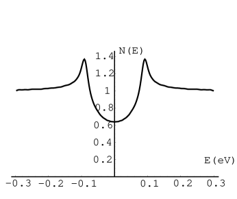
FIG. 4.: Density of states of a $(10,10)$ crystal. A pseudogap of about $0.09$ eV develops at the Fermi level.

IV Compositional Disorder

A compositionally disordered rope contains a random distribution of chiral tubes. Since tubes with different chiralities have different periodicities, Bloch’s theorem is of little use for describing the eigenstates of the entire rope. Nonetheless, in the absence of coupling between the tubes, we know that the eigenstates on each tube are plane waves. Our approach is to describe the coupling between these plane waves perturbatively. We begin by considering the simpler problem of the electronic structure of two coupled nanotubes of different chirality.

A Coupling between two tubes of different chirality

The electronic coupling between two tubes of different chirality conserves the momentum along the tube up to reciprocal lattice vectors in either tube. As we have argued in section II, the sum over reciprocal lattice vectors is dominated by the terms in which ${\bf k}+{\bf G}$ are near the first star of ${\bf K}$ points. When the coupling between the tubes is weak, it is useful to view this as momentum conserving coupling between states located near the three equivalent ${\bf K}$ points. It must be kept in mind that two states ${\bf K}_{0}+{\bf q}$ and ${\bf K}_{1}+{\bf q}$ in the vicinity of different ${\bf K}$’s are actually the same state.

Fig. 5 shows the Brillouin zones of two nanotubes with chiral angles $\theta_{a}$ and $\theta_{b}$ oriented so that the $u_{a}$ and $u_{b}$ axes coincide. Since the tunneling Hamiltonian conserves $k_{u}$, it is convenient to view the band structure of the pair of tubes as a function of $k_{u}$. Consider first the band structure in the absence of coupling. The solid bands describe the low energy states on one tube, while the dotted ones show the states on the other tube. Each set of bands is replicated three times, reflecting the three equivalent ${\bf K}$ points. In Fig. 6 we show the band structure in the vicinity of the Fermi points with the minimum momentum mismatch, for the uncoupled system(Fig. 6a), and for the couple one(Fig. 6b). To lowest order, the effect of the coupling is only important near points of degeneracy, i.e. where we have band crossing. This occurs in two cases. The first, which we refer to as a “backscattering gap” occurs when the right and left moving bands on each tube cross. The second, which we refer to as a “tunneling gap” occurs when the left moving band on one tube crosses the right moving band on the other tube.

FIG. 5.: Brillouin zones of two tubes of different chiralities. The zones are rotated such that the $u_{a}$ and $u_{b}$ axes coincide. In the lower part of the figure we show the low energy band structure of the two metallic tubes. Solid bands belong to one tube while dotted ones belong to the other one. The bands are replicated three times, reflecting the three equivalent $K$ points.

The effect of the coupling depends on two crucial energy scales: (1) the tunneling matrix element, $t$, which we estimated in (2.27) to be less than 7.5 meV, and (2) the energy mismatch

$$\Delta E=v[\alpha_{a}({\bf K}_{a\ell_{a}})_{u}-\alpha_{b}({\bf K}_{b\ell_{b}})_{u}],$$ (51)

which determines the energy at which the right and left moving bands on tubes $a$ and $b$ cross. In general, this energy mismatch depends on the chiral angles $\theta_{a}$ and $\theta_{b}$ of the two tubes as well as the Fermi point indices $i$ and $j$. In Fig. 7 we show the variation of the energy mismatch $\Delta E$ with the tube chirality for all the metallic tubes with diameters between $1.2-1.5$ nm. Tubes which are mirror images to one another have the same diameter and energy difference. The offset of the $u$ momentum is taken at a zigzag tube; in that case an (18,0) tube. As we see the typical energy mismatch is a few hundred meV. The fact that $t\ll\Delta E$ simplifies the problem considerably and justifies our perturbative approach. Of course it breaks down in special cases when $\Delta E$ is zero or very small, which occurs, for instance when the two tubes are mirror images of each other.

FIG. 6.: (a) Band structure of the two(uncoupled) tubes in the vicinity of the Fermi point with the minimum momentum mismatch $\Delta k$, which defines the important energy scale $\Delta E=v\Delta k$. (b) Band structure of the coupled tubes near the Fermi energy. Backscattering gaps open quadratically with the tunneling strength $t$, whereas tunneling gaps are linear in $t$. In general, backscattering gaps open at different energies.

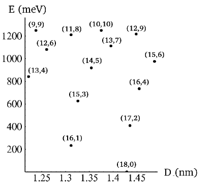
FIG. 7.: A plot showing the minimum energy mismatch $\Delta E$ for different metallic tubes with radii lying between $1.2$ and $1.5$ nm. The energy offset is taken at a zigzag tube$(18,0)$

The tunneling Hamiltonian couples left and right movers in first order, and therefore the tunneling gap is linear in the tunneling strength $t$. The gap opens at $\Delta E/2$ and since $t$ is much smaller than $\Delta E$, one concludes that tube-tube coupling has a small effect near the Fermi energy.

Backscattering gaps form through second order coupling between left and right movers on the same tube, and hence the gap is second order in the tunneling strength; $E_{g}\sim t^{2}/\Delta E$, which is of order $1$ meV. Furthermore, because the tunneling matrix elements are not invariant under the interchange of the two tubes, the backscattering gap of each tube opens at a different energy. This means that the effect on the density of states near the Fermi energy is weakened by the wiggling of the gaps. In what follows, we present quantitative arguments justifying our expectations.

We focus first on the tunneling gaps. The movers on each tube couple in first order. In general, crossing occurs at three different energies, as dictated by the momentum mismatch between the Fermi points of the two tubes(see Fig. 5). Since we are ultimately interested in the effect of tube interactions on the states nearest to the Fermi level, we only consider points with the lowest lying crossing. We denote these by $\alpha_{a}{\bf K}_{ai}$ and $\alpha_{b}{\bf K}_{bj}$. To find the magnitude of the gaps and their offsets we need to diagonalize the first order perturbation matrix. We thus consider the Hamiltonian which couples the right moving states on tube $a$ with the left moving states on tube $b$, and we diagonalize the matrix

$${\cal H}^{T}_{a}=\left[\begin{array}[]{*2c}v({\bf q}-\alpha_{a}{\bf K}_{ai})_{u}&T^{\prime}(\alpha_{a}R{\bf q}_{a}|\alpha_{b}L{\bf q}_{b})\\ T^{\prime*}(\alpha_{a}R{\bf q}_{a}|\alpha_{b}L{\bf q}_{b})&-v({\bf q}-\alpha_{b}{\bf K}_{bj})_{u}\\ \end{array}\right],$$ (52)

where ${\bf q}$ is measured from the Fermi point of tube $a$. For $\alpha_{a},\alpha_{b}=+1$ the magnitude of the tunneling gap is

$$E^{T}_{g}=2|T^{\prime}_{RL}|=4t_{T}e^{-{1\over 4}Ra_{0}K_{0}^{2}(\sin\omega_{ai}+\sin\omega_{bj})^{2}}\Big{|}\cos{\omega_{ai}\over 2}\sin{\omega_{bj}\over 2}\Big{|}.$$ (53)

It is centered about an energy $E^{T}_{o}=\Delta E/2$ above the Fermi energy. Notice that the $+$ sign in the argument of the exponential is due to the fact that the tubes face each other from the outside. As we see from Fig. 7, the average energy separation $\Delta E\sim 300$ meV, whereas the tunneling gap $E^{T}_{g}<30$ meV. This means that in a rope with a random distribution of chiralities, the opening of such gaps will have a negligible effect near the Fermi level.

Now we focus on the backscattering gaps which form near the Fermi level. Since the left and right moving states on the same tube do not couple in first order, we use second order degenerate perturbation theory. We are interested in calculating the size of the resulting gap as well as the offset of the gap. In order to calculate these, we need to diagonalize the matrix which arises from the second order coupling between the states. In general, we have tunneling between all Fermi points on each tube. Since the magnitude of the backscattering gaps varies quadratically with the tunneling strength and inversely with the energy difference $\Delta E$, the most effective contributions are those with the highest tunneling strength and lowest $\Delta E$. This argument makes us only include the set of nearest ${\bf K}$ points. Therefore, we diagonalize

$${\cal H}^{a}=\left[\begin{array}[]{*2c}v({\bf q}-\alpha_{a}{\bf K}_{a0})_{u}+E_{RR}^{a}&E_{RL}^{a}\\ E_{LR}^{a}&-v({\bf q}-\alpha_{a}{\bf K}_{a0})_{u}+E_{LL}^{a}\\ \end{array}\right],$$ (54)

where

$$E_{\lambda\lambda^{\prime}}^{a}=\sum_{<\ell_{a}\ell_{b}>}\frac{\Big{[}T^{\prime}(\alpha_{a}\lambda{\bf q}_{a}|\alpha_{b}L{\bf q}_{b})T^{\prime*}(\alpha_{a}\lambda^{\prime}{\bf q}_{a}|\alpha_{b}L{\bf q}_{b})-T^{\prime}(\alpha_{a}\lambda{\bf q}_{a}|\alpha_{b}R{\bf q}_{b})T^{\prime*}(\alpha_{a}\lambda^{\prime}{\bf q}_{a}|\alpha_{b}R{\bf q}_{b})\Big{]}}{v(\alpha_{a}{\bf K}_{a\ell_{a}}-\alpha_{b}{\bf K}_{b\ell_{b}})_{u}}\Bigg{|}_{{\bf q}_{a}=0},$$ (55)

and $\lambda,\lambda^{\prime}=R,L$.

Diagonalizing, we get

$$E_{\pm}^{a}({\bf q})=\frac{E_{LL}^{a}+E_{RR}^{a}}{2}\pm\sqrt{\bigg{(}v({\bf q}-\alpha_{a}{\bf K}_{a0})_{u}-\frac{E_{LL}^{a}-E_{RR}^{a}}{2}\bigg{)}^{2}+|E_{RL}^{a}|^{2}}.$$ (56)

The backscattering gap is $E_{g}^{a}=2|E_{RL}^{a}|$, and it opens around an energy offset $E_{o}^{a}=(E_{RR}^{a}+E_{LL}^{a})/2$. We thus find

$$E_{g}^{a}={4t_{T}^{2}\over vK_{0}}\bigg{|}\sum_{<\ell_{a}\ell_{b}>}{e^{-{1\over 2}Ra_{0}K_{0}^{2}(\alpha_{a}\sin\omega_{a\ell_{a}}+\alpha_{b}\sin\omega_{b\ell_{b}})^{2}}\over\alpha_{a}\cos\omega_{a\ell_{a}}-\alpha_{b}\cos\omega_{b\ell_{b}}}\sin\omega_{a\ell_{a}}\cos\omega_{b\ell_{b}}\bigg{|},$$ (57)

and

$$E_{o}^{a}={2t_{T}^{2}\over vK_{0}}\sum_{<\ell_{a}\ell_{b}>}{e^{-{1\over 2}Ra_{0}K_{0}^{2}(\alpha_{a}\sin\omega_{a\ell_{a}}+\alpha_{b}\sin\omega_{b\ell_{b}})^{2}}\over\alpha_{a}\cos\omega_{a\ell_{a}}-\alpha_{b}\cos\omega_{b\ell_{b}}}\cos\omega_{b\ell_{b}}.$$ (58)

Eqs(4.7) and (4.8) show that, in general, the gap offset $E_{o}$ is greater than the gap $E_{g}$. In addition, one expects that the offsets and gaps of both tubes will generally be different. This means that the gaps wiggle around the Fermi energy as the chiral angle is changed, leading to the conclusion that in a rope formed of a random collection of chiralities, the effect on the density of states around $E_{F}$ is very small.

Let us now have a closer look at the contributions of different tunneling points. In general, only one set of Fermi points will dominate, unless the tubes are mirror images of each other. We now argue that in a case when the tubes have different chiralities, it is a certain set of Fermi points that is actually important.

We want to understand which tubes significantly couple to each other, and for those tubes, the Fermi points at which the coupling is most effective. To do this, we study the quantity

$${t\over\Delta E}={t_{T}\over vK_{0}}{e^{-{1\over 4}Ra_{0}K_{0}^{2}(\alpha_{a}\sin\omega_{a\ell_{a}}+\alpha_{b}\sin\omega_{b\ell_{b}})^{2}}\over\alpha_{a}\cos\omega_{a\ell_{a}}-\alpha_{b}\cos\omega_{b\ell_{b}}}.$$ (59)

This quantity will be dominated by the exponential factor, and in cases where different sets of points have nearly equal exponential contribution, the denominator will dominate.

For nearly armchair tubes, the maximum is at $\omega_{a(b)\ell(\ell^{\prime})}\sim 0$, i.e., around the ${\bf K}_{0}$ points(${\bf K}_{0}{\mbox{-}}{\bf K}_{0}$ tunneling). In that case, the exponential factor is approximately $1$, and the denominator takes it minimum value($\sim 7$ meV) as the two $\omega$’s are closest to zero. As the tubes shift from being armchair, the denominator increases as the Fermi points rotate away from the $u$ axis, thereby making the tunneling less effective.

For tubes which are nearly mirror images of each other, the dominant set is also the ${\bf K}_{0}{\mbox{-}}{\bf K}_{0}$. While moving away from the armchair region does not significantly change the exponential contribution, it makes the denominator bigger, hence making the coupling less important.

For tubes which are nearly zigzag(but are not mirror images of each other), tunneling is the least effective, as both the exponential argument and the denominator are big. In some of these cases, ${\bf K}_{0}{\mbox{-}}{\bf K}_{0}$ tunneling may not be the dominant one.

We thus conclude that tunneling is most effective between tubes which are nearly armchair, and that the ${\bf K}_{0}{\mbox{-}}{\bf K}_{0}$ tunneling is the most important one, and hence $E_{RR}^{1}$(and similar sums) are dominated by one term. In other words, the sum over reciprocal lattice vectors in the tunneling Hamiltonian is dominated by a single term. If we ignore the other terms, then there is no reciprocal lattice vector sum, and the system effectively has translational invariance in the direction parallel to the tubes. This “dominant Fermi point approximation” simplifies our problem considerably, since it allows us to assign a conserved momentum to each state. This will allow us to compute the band structure for an entire rope in the following section.

B Compositionally disordered rope

In this section we study the electronic structure of a nanotube rope composed of tubes with a random distribution of diameters and chiralities. We expect that the momentum mismatch between the Fermi points of neighboring tubes will suppress the tunneling and lead to localization. In real ropes, we expect $2/3$ of the tubes to be semiconducting. As indicated in Fig. 8, this will make the localization effects even stronger. To emphasize our point, we consider a compositionally disordered rope with only metallic tubes.

FIG. 8.: (a) A compositionally disordered metallic rope. Different gray scales indicate different tube chiralities. (b) A compositionally disordered rope with $1/3$ of its tubes metallic. The vacant circles denote semiconducting tubes. It is clear that the semiconducting tubes percolate along the rope.

To solve the problem, we employ the “dominant Fermi point approximation” introduced in the preceding section. In this approximation, the momentum $k=K_{0u}+q$ is conserved by the tunneling Hamiltonian. We may thus write

$${\cal H}=\sum_{i}{\cal H}_{i}+\sum_{<ij>}{\cal H}_{ij},$$ (60)

with

$${\cal H}_{i}=\sum_{\alpha k}v(k-\alpha K_{0u}^{i})(\psi^{\dagger}_{i\alpha kR}\psi_{i\alpha kR}-\psi^{\dagger}_{i\alpha kL}\psi_{i\alpha kL}),$$ (61)

and

$${\cal H}_{ij}=\sum_{\alpha\eta^{\prime}_{i}\eta^{\prime}_{j}k}\widetilde{T^{\prime}}(\alpha\eta^{\prime}_{i}|\alpha\eta^{\prime}_{j})\psi_{i\alpha k\eta^{\prime}_{i}}^{\dagger}\psi_{j\alpha k\eta^{\prime}_{j}},$$ (62)

where $\widetilde{T^{\prime}}$is the tunneling matrix given by

$$\widetilde{T^{\prime}}=2t_{T}e^{-{1\over 4}Ra_{0}K_{0}^{2}(\sin\omega_{i0}+\sin\omega_{j0})^{2}}\left[\begin{array}[]{*2c}\cos{\omega_{i0}\over 2}\cos{\omega_{j0}\over 2}&i\cos{\omega_{i0}\over 2}\sin{\omega_{j0}\over 2}\\ -i\sin{\omega_{i0}\over 2}\cos{\omega_{j0}\over 2}&\sin{\omega_{i0}\over 2}\sin{\omega_{j0}\over 2}\end{array}\right].$$ (63)

The Hamiltonian may now be diagonalized for each $k$ by diagonalizing a $4N\times 4N$ matrix, where $N$ is the number of tubes in the rope. For each $k$, the $m^{\mbox{th}}$ eigenstate may be described by a “wavefunction” $\zeta^{m}_{\alpha\eta}(i)$, which is the amplitude for the particle to be in state $\alpha$, $\eta$ on tube $i$.

A portion of the band structure of the metallic rope is shown in Fig. 9a. It is clear that there is no significant change in the vicinity of the Fermi energy. As we have argued before the backscattering gaps wiggle around the Fermi energy, thereby negligibly changing the density of states, which is shown in Fig. 9b. Therefore, no pseudo gap develops.

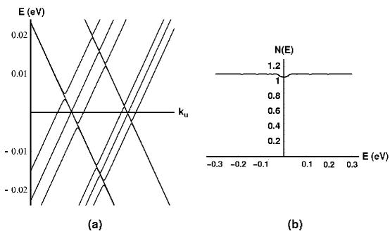
FIG. 9.: (a) Low energy band structure of a compositionally disordered metallic rope, showing tunneling and backscattering gaps. The latter wiggle around the Fermi energy, leading to a negligible effect on the density of states, which is shown in (b).

The extent of localization of the eigenstates may be quantitatively measured by computing the correlation function

$$C(r_{\perp},E)=\sum_{ijm\alpha\eta\alpha^{\prime}\eta^{\prime}}|\zeta^{m}_{\alpha\eta}(i)|^{2}|\zeta^{m}_{\alpha^{\prime}\eta^{\prime}}(j)|^{2}\delta(|{\bf R}_{i}-{\bf R}_{j}|-r_{\perp})\delta(E_{m}-E),$$ (64)

at the Fermi energy, where ${\bf R}_{i}$ is the position of tube $i$ in the rope. As shown in Fig. 10, the correlation function decays exponentially with distance, $C(r_{\perp},E_{F})\propto e^{-2r_{\perp}/\xi_{\perp}}$, indicating that the eigenstates are localized perpendicular to the tube axes with a localization length $\xi_{\perp}\sim 10{\mbox{\AA}}$. Thus the eigenstates are predominantly on a single tube.

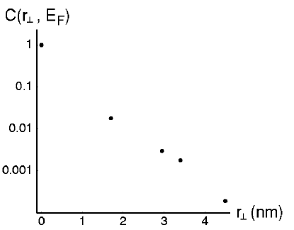
FIG. 10.: The correlation function $C(r_{\perp},E_{F})$ defined by eq(4.14), which gives a quantitative measure of the localization of the states on single tubes.

V Conclusion

In this paper we have shown that the constraints of energy and crystal momentum conservation severely restrict the electronic coupling between carbon nanotubes. The electronic coupling between two nanotubes is only effective when the eigenstates near the Fermi energy have the same momentum, which requires that the graphene sheets of the two nanotubes are oriented parallel to one another. This only occurs when the two tubes are mirror images of one another. Thus, in contrast to a crystalline rope of armchair nanotubes, in which eigenstates are extended throughout the rope, we find that the electronic eigenstates of a compositionally disordered rope are strongly localized on individual nanotubes.

This conclusion has important consequences for the transport properties of nanotube ropes. In particular, it provides a natural explanation of the nonlocal effects observed by Bockrath et al. [9] in their multi-terminal conductance measurements. These effects can arise when different electrical leads make contact to different tubes within a rope, allowing the current in a tube to “bypass” an electrical lead which it does not contact.

In the absence of impurities, the eigenstates will be localized on a single tube, but extend across the entire length of a tube. Scattering, either due to impurities or tube ends, will tend to localize the states in the tube direction. Paradoxically, by relaxing the constraint of momentum conservation such scattering will increase the coupling between tubes. Nonetheless, we are led to a picture of highly anisotropic localization.

This picture may help to explain some apparently paradoxical transport data on nanotube mats. At low temperatures, nanotube mats are observed to obey the three dimensional Mott variable range hopping law, $R=R_{0}\exp(T_{0}/T)^{1/4}$, with $T_{0}$ of order 100 K [10]. If one uses the standard formula for isotropic variable range hopping and knowledge of the nanotube’s density of states, one extracts a localization length of order $200$Å. By contrast, Fuhrer et al. [11] have analyzed the scaling of the hopping conductivity with electric field and temperature $R(E,T)=f(\xi E/T)$, and have argued that the localization length is much longer, of order 6000Å. Our picture of anisotropic localization offers a possible resolution to this discrepancy. In the simplest model of anisotropic variable range hopping, $T_{0}$ depends on the geometric mean of the localization lengths, $(\xi_{\parallel}\xi_{\perp}^{2})^{1/3}$, while the scaling with electric field depends on the longest localization length, $\xi_{\parallel}$.

In this paper, we have developed a general framework for describing the electronic coupling between graphene based structures. This approach should prove useful for other problems, including the coupling between neighboring shells of multiwalled tubes as well as the coupling between crossed single walled tubes. Analysis of these problems will be left for future work.

A Lattice Fourier Transforms

In this appendix, we work out explicitly the Fourier transform in section IIA. As shown in Fig. 1 the positions of the lattice may be written as ${\bf r}_{i}={\bf R}+{\bf\rho}+\eta{\bf\tau}$, which may be specified by a lattice vector ${\bf R}$, and a sublattice index $\eta=\pm 1$. The position of the center of the hexagon is given by $\rho$. Consider first a sum over lattice sites of the form

$${1\over\sqrt{N}}\sum_{i}f({\bf r}_{i})e^{-i{\bf k}\cdot{\bf r}_{i}}={1\over\sqrt{N}}\sum_{{\bf R}\eta}f({\bf r})e^{i{\bf k}\cdot{\bf r}}|_{{\bf r}={\bf R}+{\bf\rho}+\eta\tau}.$$ (A1)

The sum over ${\bf R}$ may be performed by introducing reciprocal lattice vectors ${\bf G}$,

$$={1\over{A_{\rm cell}\sqrt{N}}}\sum_{{\bf G}\eta}\int d^{2}re^{-i{\bf G}\cdot({\bf r}-\rho-\eta\tau)}f({\bf r})e^{-i{\bf k}\cdot{\bf r}}.$$ (A2)

Defining the Fourier transform,

$$f_{\bf k}={1\over{A_{\rm cell}\sqrt{N}}}\int d^{2}rt({\bf r})e^{-i{\bf k}\cdot{\bf r}},$$ (A3)

we may then write

$${1\over\sqrt{N}}\sum_{i}f({\bf r}_{i})e^{-i{\bf k}\cdot{\bf r}_{i}}=\sum_{{\bf G}\eta}e^{i{\bf G}\cdot{\bf d}_{\eta}}f_{{\bf G}+{\bf k}}.$$ (A4)

REFERENCES

- [1] A. Thess et al., Science 273, 483 (1996).
- [2] R. Saito, M. Fujita, G. Dresselhaus and M.S. Dresselhaus, Appl. Phys. Lett. 60, 2204 (1992); J.W. Mintmire, D.H. Robertson and C.T. White, J. Phys. Chem. Solids 54, 1835 (1993); N. Hamada, S. Sawada, and A. Oshiyama, Phys. Rev. Lett. 69, 1579 (1992); J.W. Mintmire, B.I. Dunlap, and C.T. White, Phys. Rev. Lett. 68, 631 (1992).
- [3] P. Kin, T.W. Odom, J.L. Huang, and C.M. Lieber, Phys. Rev. Lett. 82, 1225 (1999); L.C. Venema et al., Science 283, 52 (1999); W. Clauss, D. Bergeron, and A.T. Johnson, Phys. Rev. B 50, R4266 (1998).
- [4] A.M. Rao et al., Science 275, 187 (1997); U.D. Venkateswaran et al., Phys. Rev. B 59, 10928 (1999).
- [5] S. Frank, P. Poncharal, Z.L. Wang, and W.A. de Heer, Science 280, 1744 (1998); A. Bachtold et al. Nature 397, 673 (1998).
- [6] C.L. Kane, E.J. Mele, Phys. Rev. Lett. 78, 1932 (1997).
- [7] S. Ergun, Chem. Phys. Carbon 3, 45 (1968).
- [8] P. Delaney et al., Nature 391, 466 (1998); Y.K. Kwon, S. Saito, and D. Tománek, Phys. Rev. B 58, R13314 (1998); J.-C. Charlier, X. Gonze, and J.-P. Michenaud, Euro. Phys. Lett. 29, 43 (1995)
- [9] M. Bockrath et al., Science 275, 1922 (1997).
- [10] R. Antonov, Ph.D. thesis, University of Pennsylvania, 1998.
- [11] M.S. Fuhrer et al., in Electronic properties of novel materials-Progress in molecular nanostructures, AIP conference proceedings 442, Kirchberg, Tyrol, Austria, 1997, p. 69.