Multiple scaling regimes in simple aging models

Abstract

We investigate aging in glassy systems based on a simple model, where a point in configuration space performs thermally activated jumps between the minima of a random energy landscape. The model allows us to show explicitly a subaging behavior and multiple scaling regimes for the correlation function. Both the exponents characterizing the scaling of the different relaxation times with the waiting time and those characterizing the asymptotic decay of the scaling functions are obtained analytically by invoking a ‘partial equilibrium’ concept.

PACS numbers: 02.50.-r, 75.10.Nr, 05.20.-y

The dynamics of glassy materials can be strongly dependent on the history of glass formation [1, 2]. Generally speaking, one finds that the relaxation dynamics becomes increasingly slower with the “age” of the system, that means with the time $t_{w}$ expired since the material was brought into the glassy state. Such aging phenomena have been identified in many systems and various dynamical probes (for a recent review, see e.g. [3]). Prominent examples are shear stress relaxations in structural glasses [4], thermoremanent magnetizations in spin glasses [5], and electric field relaxations in dipolar glasses [6]. A convenient way to quantify aging in such experiments is to disturb the probe at time $t_{w}$ by a sudden change of external field, and to measure the response $R(t_{w}+t,t_{w})$ at a later time $t_{w}+t$. Often, the characteristic relaxation time grows proportionally to the age $t_{w}$. When $t$ is larger than all microscopic times associated with fast time-translational invariant relaxations, one then expects $R(t_{w}+t,t_{w})$ to depend on the ratio $t/t_{w}$ only, i.e. $R(t_{w}\!+\!t,t_{w})=F(t/t_{w})$.

In principle, however, one cannot rule out other scaling forms, as e.g. $R(t_{w}\!+\!t,t_{w})=F(t/t_{w}^{\mu})$ with $\mu>0$ being different from one. In particular the case $\mu<1$, which has been called ‘subaging’ because the effective relaxation time grows more slowly than the age of the system, seems to be of experimental relevance [3]. It is moreover possible that there exist, for given waiting time $t_{w}$, various scaling regimes in time $t$, which are governed by different relaxation times $\propto t_{w}^{\mu_{s}}$, $s=1,2,\ldots$. More precisely, depending on how $t$ is scaled with $t_{w}$, one can obtain different asymptotic scaling functions in the limit $t_{w}\!\to\!\infty$. For example, for $\mu_{1}\!>\!\mu_{2}\!>\!0$, one may find $R(t_{w}\!+\!\Lambda_{1}\,t_{w}^{\mu_{1}},t_{w})\!\sim\!F_{1}(\Lambda_{1})$ and $R(t_{w}\!+\!\Lambda_{2}\,t_{w}^{\mu_{2}},t_{w})\!\sim\!F_{2}(\Lambda_{2})$ when $t_{w}\to\infty$. In fact, the occurrence of different scaling functions being associated with various time regimes has recently been conjectured on the basis of analytical results for the Langevin dynamics of mean-field spin glass models [7, 3]. So far, however, it was not possible to validate these conjectures, or to exemplify them in some reasonable phenomenological models.

In this Letter we will discuss a model that allows us to demonstrate for the first time explicitly the possible occurrence of subaging behavior and multiple scaling regimes. This model, which has a strong resemblance to the previously studied “trap model” [8, 9], is motivated by the simple and widespread view that glassy dynamics may be described by a thermally activated motion of a point (“particle”) that jumps among the deep (free) energy minima $E_{i}$ of a complex configuration space. According to extreme value statistics one may expect the distribution $\rho(E)$ of these deep minima to be exponential, and indeed, mean-field theories of spin glasses [10] and recent results from molecular dynamics simulations [11] suggest this to be the case.

To be specific, let us consider a $d$-dimensional cubic lattice and assign to each lattice site $i$ an energy $E_{i}$, $-\infty\!<\!E_{i}\!\leq\!0$, drawn from the distribution $\rho(E)\!=\!T_{\rm g}^{-1}\exp(E/T_{\rm g})$. The particle jumps among nearest neighbor sites only, and the jump rate from site $i$ to a neighboring site $j$ is

$$w_{i,j}=\nu\exp\left(-\beta[\alpha E_{j}-(1-\alpha)E_{i}]\right)\,,$$ (1)

where the “attempt frequency” $\nu\!\equiv\!1$ sets our time unit, $\beta^{-1}\!\equiv\!T$ is the temperature (or thermal energy), and the parameter $\alpha$ specifies how the energies of the initial and target site are weighted. In order for the $w_{i,j}$ to obey detailed balance, $\alpha$ can assume any real value, but on physical grounds it is reasonable to restrict $\alpha$ to the range $0\!\leq\!\alpha\!\leq\!1$. Independent of $\alpha$, the system undergoes a “dynamical phase transition” at $T\!=\!T_{\rm g}$: In the high-temperature phase, where $T\!>\!T_{\rm g}$, the probability $\varphi(E)\!\propto\!\rho(E)\exp(-\beta E)$ for finding the system in a state with energy $E$ is normalizable and thermal equilibrium will be approached with a characteristic equilibration time that diverges for $T\!\searrow\!T_{\rm g}$. By contrast, in the glassy phase, where $T\!<\!T_{\rm g}$ and $\varphi(E)$ is not normalizable, the dynamics never becomes stationary but ‘ages’.

It is important at this point to stress the differences between the above model and the earlier studied trap model [8]. In the latter, the jump rates depend only on the energy of the initial site corresponding to $\alpha\!=\!0$ in eq. (1), and this allows a straightforward mapping onto a continuous time-random walk with a waiting time distribution decaying as a power law. Much more important,

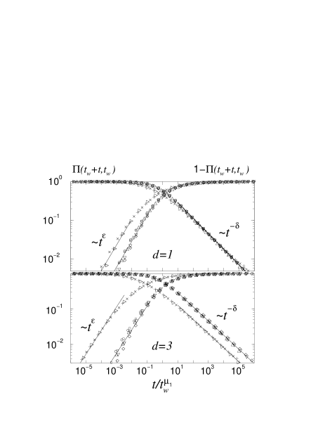
FIG. 1.: Double-logarithmic plot of $\Pi(t_{w}\!+\!t,t_{w})$, $1-$ $\Pi(t_{w}\!+\!t,t_{w})$ (symbols $\circ,\,{\scriptstyle\square},\,{\scriptstyle\triangle},\,\triangledown,\,\diamond$) and $\tilde{\Pi}(t_{w}\!+\!t,t_{w})$, $1\!-\!\tilde{\Pi}(t_{w}\!+\!t,t_{w})$ (symbols $\triangleright,\,+,\,\times$) as functions of $t/t_{w}^{\mu_{1}}$ in $d\!=\!1$ and $d\!=\!3$ for $(\theta,\alpha)\!=\!(1/4,3/8)$. Different symbols correspond to different waiting times, $t_{w}\!=\!10^{5}$ ($\diamond$), $10^{6}$ ($\triangledown$), $10^{7}$ (${\scriptstyle\triangle}$), $10^{8}$ (${\scriptstyle\square}$), $10^{9}$ ($\circ$) and $t_{w}\!=\!10^{8}$ ($\triangleright$), $10^{11}$ ($+$), $10^{13}$ ($\times$) in $d=1$, as well as $t_{w}\!=\!10^{6}$ ($\diamond$), $10^{7}$ ($\triangledown$), $10^{8}$ (${\scriptstyle\triangle}$), $10^{9}$ (${\scriptstyle\square}$), $10^{10}$ ($\circ$) and $t_{w}\!=\!10^{11}$ ($\triangleright$), $10^{13}$ ($+$), $10^{15}$ ($\times$) in $d=3$. The solid lines have slope $\epsilon$ (small $t$ behavior) and slope $-\delta$ (large $t$ behavior). For the value of the exponents $\epsilon$ and $\delta$, see text.

the trap model was so far considered only on a mean-field level corresponding to an “annealed situation”, where the site energies are drawn anew after each jump.

In order to study aging effects in the glassy phase, we focus, as in the trap model, on the (disorder averaged) probability $\Pi(t_{w}\!+\!t,t_{w})$ that the system does not change its state between $t_{w}$ and $t_{w}+t$. For particles hopping on a lattice, this can be interpreted as a dynamical structure factor [8]. Initially, the particle is located on any of the sites and then it starts to explore the configuration space at some $T\!<\!T_{\rm g}$. Physically, this means that we are considering an instantaneous quench from $T=\infty$.

Our idea to explore the scaling properties of $\Pi(t_{w}\!+\!t,t_{w})$ for both $t$ and $t_{w}$ becoming large is based on the following “partial equilibrium” concept: From the time after the quench up to $t_{w}$ the particle has followed a Brownian path in configuration space that on average consists of $S(t_{w})$ distinct and mutually connected sites. On a typical path with $S\simeq S(t_{w})$ sites then, it is reasonable to think that the particles should effectively equilibrate, i.e. the probability to be on a particular site $j$ of the path may be approximated by $\tau_{j}/\sum_{k=1}^{S}\tau_{k}$, where $\tau_{j}\equiv\exp(-\beta E_{j})$ ($1\!\leq\!\tau_{j}\!<\infty$). Conditioned on being at the site $j$, the system has a probability $\exp(-t\sum_{n_{j}}w_{j,n_{j}})=\exp(-t\,\tau_{j}^{\alpha-1}\sum_{n_{j}}\tau_{n_{j}}^{\alpha})$ not to change state within time $t$, where the sum over $n_{j}$ runs over all nearest neighbor sites of $j$. Exactly two of these neighboring sites are considered to belong to the Brownian path in view of its one-dimensional topology. The remaining $2(d\!-\!1)$ neighboring sites are assumed to have not been visited before. Hence, we may deduce the scaling properties of $\Pi(t_{w}\!+\!t,t_{w})$ from

$$\tilde{\Pi}(t_{w}\!+\!t,t_{w})\!\equiv\!\left\langle\frac{\sum_{j=1}^{S(t_{w})}\tau_{j}\exp\Bigl{(}-t\,\tau_{j}^{\alpha-1}\sum_{n_{j}}\tau_{n_{j}}^{\alpha}\Bigr{)}}{\sum_{k=1}^{S(t_{w})}\tau_{k}}\right\rangle,$$ (2)

where $\langle\ldots\rangle$ denotes an average over $(2d-1)S(t_{w})$ uncorrelated random numbers $\tau_{j}$ that are distributed according to the power law $\phi(\tau)=\theta\tau^{-1-\theta}$ with $\theta\!\equiv\!T/T_{\rm g}$.

Clearly, the partial equilibrium concept is an approximation that needs to be tested. To this end we have determined $\Pi(t_{w}+t,t_{w})$ and $S(t_{w})$ in $d\!=\!1,3$ for various values of $\theta$ and $\alpha$ by Monte Carlo simulations. Then we took $S(t_{w})$ from these simulations to calculate $\tilde{\Pi}(t_{w}\!+\!t,t_{w})$ from eq. (2). The disorder average in this simple numerical evaluation was performed over a set of realizations independent of the ones taken in the simulations.

Figure 1 shows the results for one representative parameter pair $(\theta,\alpha)\!=\!(1/4,3/8)$. The data have been collected as functions of $t$ for a broad range of fixed waiting times $t_{w}$ and are plotted already in scaled form as functions of $\Lambda_{1}=t/t_{w}^{\mu_{1}}$ with exponents $\mu_{1}\!=\!\mu_{1}(\theta,\alpha)$ being specified below. As can be seen from the figure, the data for both $\Pi(t_{w}\!+\!t,t_{w})$ and $\tilde{\Pi}(t_{w}\!+\!t,t_{w})$ collapse onto single curves $F_{1}(\Lambda_{1})$ and $\tilde{F}_{1}(\Lambda_{1})$, respectively. Although the two scaling functions are different, their asymptotic behavior for large $\Lambda_{1}$ is the same, $F_{1}(\Lambda_{1})\sim\tilde{F}_{1}(\Lambda_{1})\sim\Lambda_{1}^{-\delta}$ (see the solid lines in Fig. 1). The values of the exponent $\delta\!=\!\delta(\theta,\alpha)$ are given below.

It is important to inspect also more closely the ‘short’ time regime, where the complementary probability $1\!-\!\Pi(t_{w}\!+\!t,t_{w})$ for the system to change state between $t_{w}$ and $t_{w}\!+\!t$ is small. This complementary probability can be as relevant as $\Pi(t_{w}\!+\!t,t_{w})$ dependent on the physical quantity being measured. Scaling plots of $1\!-\!\Pi(t_{w}\!+\!t,t_{w})$ and $1\!-\!\tilde{\Pi}(t_{w}\!+t,t_{w})$ as functions of $\Lambda_{1}=t/t_{w}^{\mu_{1}}$ in $d\!=\!1,3$ are also shown in Fig. 1. Again there is a good data collapse and for $\Lambda_{1}\to 0$ we find $1\!-\!F_{1}(\Lambda_{1})\sim 1\!-\!\tilde{F}_{1}(\Lambda_{1})\sim\Lambda_{1}^{\epsilon}$ with exponents $\epsilon=\epsilon(\theta,\alpha)$ given below. An analogous overall behavior as displayed in Fig. 1 was found also for other pairs $(\theta,\alpha)$ (with $0\!<\theta\!<\!1$, $0\!\leq\!\alpha\!\leq\!1$). We thus conclude that the partial equilibrium concept not only yields the correct scaling behavior (same $\mu_{1}$ exponents) but also the correct asymptotics of the scaling functions [12]. However, a study of the ‘participation ratios’ (see [13] for their definition) shows that the partial equilibrium concept is not exact, even for large times [14].

Now we turn to the analytical study of eq. (2). Since $\tilde{\Pi}(t_{w}\!+\!t,t_{w})$ depends on $t_{w}$ only via $S(t_{w})$ let us first discuss the scaling of $S(t_{w})$ with time $t_{w}$. For $\alpha\!=\!0$ this problem has been addressed some time ago (see e.g. [15]) and for $t_{w}\!\to\!\infty$ one finds

$$S(t_{w})\sim t_{w}^{\gamma}\,,\hskip 8.5359pt\gamma=\left\{\begin{array}[]{cl}\displaystyle\frac{d\,\theta}{d\!+\!(2\!-\!d)\theta}\,,&1\leq d<2\\ \theta\,,&d>2\end{array}\right.$$ (3)

(In $d\!=\!2$ there are logarithmic corrections, $S(t_{w})\sim[t_{w}/\log t_{w}]^{\theta}$.) For $0\!<\!\alpha\!\leq\!1$ one expects (3) not to change, since $\alpha$ only affects the nearest-neighbor hopping rates but not the transport properties on large length scales. In fact, in our simulations we always found eq. (3) to hold true. Let us note also that in $d\!=\!1$ one can give a simple finite-size scaling argument to show that (3) remains valid for $0\!<\!\alpha\!\leq\!1$.

Next we derive the scaling properties of $\tilde{\Pi}$ as a function of $t$ and $S=S(t_{w})$, and then use eq. (3) to obtain the corresponding scaling properties of $\tilde{\Pi}$ as a function of $t$ and $t_{w}$. When replacing the denominator in eq. (2) by $\int_{0}^{\infty}d\lambda\,\exp(-\lambda\sum_{k=1}^{S}\tau_{k})$, the average over the $\tau_{j}$ can to a large extent be factorized, and one obtains the following asymptotic formula valid in the limit of large $S$

$$\tilde{\Pi} \cong \frac{\theta^{3}\tilde{S}}{\kappa}\int_{0}^{\infty}d\lambda\,e^{-\lambda^{\theta}\tilde{S}}\int_{1}^{\infty}\frac{d\tau_{1}}{\tau_{1}^{1+\theta}}\,e^{-\lambda\tau_{1}}\int_{1}^{\infty}\frac{d\tau_{2}}{\tau_{2}^{1+\theta}}\,e^{-\lambda\tau_{2}}$$ (6)

$$\times\int_{1}^{\infty}\frac{d\tau}{\tau^{\theta}}\,e^{-\lambda\tau}\Bigl{[}f\bigl{(}\frac{t}{\tau^{1-\alpha}}\bigr{)}\Bigr{]}^{2(d\!-\!1)}\exp\Bigl{(}-t\frac{\tau_{1}^{\alpha}\!+\!\tau_{2}^{\alpha}}{\tau^{1-\alpha}}\Bigr{)}\,,$$

$$f(x)\equiv\theta\int_{1}^{\infty}\frac{d\tau}{\tau^{1\!+\!\theta}}\,\exp(-x\tau^{\alpha})\,.$$

Here $\kappa\equiv\Gamma(1\!-\!\theta)$, where $\Gamma(.)$ is the Gamma function, and $\tilde{S}\equiv\kappa S$. Note that for $t\!=\!0$ and $\tilde{S}\!\to\!\infty$, eq. (6) yields the correct normalization $\tilde{\Pi}\!\to\!1$.

After two transformations $\lambda\!\to\!\tilde{S}\lambda^{\theta}$ and $\tau\!\to\!\tilde{S}^{1/\theta}\tau$ we can identify $\Lambda_{1}\!=\!t/\tilde{S}^{(1\!-\!\alpha)/\theta}$ as a scaling variable corresponding to a first characteristic time $t_{1}\!\sim\!\tilde{S}(t_{w})^{(1\!-\!\alpha)/\theta}\sim t_{w}^{\gamma(1\!-\!\alpha)/\theta}\equiv t_{w}^{\mu_{1}}$. We thus obtain

$$\mu_{1}=\frac{\gamma(1-\alpha)}{\theta}$$ (7)

with $\gamma$ from eq. (3). This exponent $\mu_{1}$ has been used to collapse the data in Fig. 1, i.e. we took $\mu_{1}=(1\!-\!\alpha)/(1\!+\!\theta)$ in $d\!=\!1$ and $\mu_{1}=(1\!-\!\alpha)$ in $d\!=\!3$. Based on the equilibrium concept it is is easy to show that $t_{1}$ has a simple physical interpretation: It scales as the typical maximum trapping time $t_{\max}(t_{w})$ encountered after $t_{w}$. In $d\!=\!1$ one thus finds a subaging behavior even for $\alpha\!=\!0$ since the deepest trap is visited a large number of times $N(t_{w})\!\sim\!t_{w}^{\theta/(1\!+\!\theta)}$, so that $t_{1}\!\sim\!t_{\max}(t_{w})\!\sim\!t_{w}/N(t_{w})\!\ll\!t_{w}$. Similarly, for $\alpha\!\neq\!0$, the deepest trap is revisited a large number of times in all dimensions $d$ due to a strong backward jump correlation when the particle leaves a site with low energy.

The scaling function in the first time domain $t\!=\!\Lambda_{1}t_{w}^{\mu_{1}}$ reads

$$\tilde{F}_{1}(\Lambda_{1}) = \frac{\theta^{3}}{\kappa}\int_{0}^{\infty}d\lambda\,e^{-\lambda^{\theta}}\int_{1}^{\infty}\frac{d\tau_{1}}{\tau_{1}^{1+\theta}}\int_{1}^{\infty}\frac{d\tau_{2}}{\tau_{2}^{1+\theta}}$$ (9)

$$\times\int_{0}^{\infty}\frac{d\tau}{\tau^{\theta}}e^{-\lambda\tau}\Bigl{[}f\bigl{(}\frac{\Lambda_{1}}{\tau^{1-\alpha}}\bigr{)}\Bigr{]}^{2(d\!-\!1)}\exp\Bigl{(}-\Lambda_{1}\frac{\tau_{1}^{\alpha}\!+\!\tau_{2}^{\alpha}}{\tau^{1-\alpha}}\Bigr{)}\,,$$

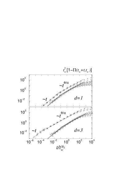
FIG. 2.: Double-logarithmic plot of $1\!-\!\Pi(t_{w}\!+\!t,t_{w})$ and $1\!-\!\tilde{\Pi}(t_{w}\!+\!t,t_{w})$ as functions of $t/t_{w}^{\mu_{2}}$ in $d\!=\!1$ and $d\!=\!3$ for the same parameters as in Fig. 1 (the same symbols have been used for the various waiting times $t_{w}$). The solid lines have slope one and $\theta/\alpha$, and indicate the limiting behavior of $F_{2}(.)$ according to eq. (15).

and has the limiting behavior

$$\tilde{F}_{1}(\Lambda_{1})\sim\left\{\begin{array}[]{lll}1-c_{\scriptscriptstyle>}\Lambda_{1}^{(1\!-\!\theta)/(1\!-\!\alpha)}\,,&\theta>\alpha&\\[-4.26773pt] &&\Lambda_{1}\to 0\\[-4.26773pt] 1-c_{\scriptscriptstyle<}\Lambda_{1}^{\theta/\alpha}\,,&\theta<\alpha&\\[7.11317pt] c_{\scriptscriptstyle\infty}\Lambda_{1}^{-\theta/(1\!-\!\alpha)}&\hskip 14.22636pt\Lambda_{1}\to\infty&\end{array}\right.$$ (10)

The constants $c_{\scriptscriptstyle>}$, $c_{\scriptscriptstyle<}$, and $c_{\scriptscriptstyle\infty}$ can be expressed in terms of $\alpha$, $\theta$ and $d$ but are not of interest here. Equation (10) yields the exponents $\delta\!=\!\theta/(1\!-\!\alpha)$ and $\epsilon\!=\!(1\!-\!\theta)/(1\!-\!\alpha)$ taken in Fig. 1 to characterize the decay of $\Pi$ and rise of $1\!-\!\Pi$, respectively. For $\alpha=0$, one recovers the results of the annealed model [8], namely $\delta\!=\!\theta$ and $\epsilon\!=\!1\!-\!\theta$.

For $\theta\!>\!\alpha$ the function $\tilde{F}_{1}(\Lambda_{1})$ describes the scaling properties of $\tilde{\Pi}$ completely. However, based on eq. (6) one finds that for $\theta\!<\!\alpha\!<\!1/2$, there exists a second scaling variable $\Lambda_{2}\!=\!t/\tilde{S}^{(1\!-\!2\alpha)/\theta}\sim t/t_{w}^{\gamma(1\!-\!2\alpha)/\theta}\equiv t/t_{w}^{\mu_{2}}$ yielding

$$\mu_{2}=\frac{\gamma(1-2\alpha)}{\theta}\,.$$ (11)

Therefore, a second characteristic time scale $t_{2}\!\sim\!S^{(1\!-\!2\alpha)/\theta}$, diverging when $t_{w}\to\infty$, governs the behavior when $\tilde{\Pi}$ is close to one. (Note that for fixed $\Lambda_{2}$, $\Lambda_{1}\!=\!\tilde{S}^{-\alpha/\theta}\Lambda_{2}\!\to\!0$ for $\tilde{S}\!\to\!\infty$). In the new time domain one finds the following generalized scaling form,

$$\tilde{S}(1-\tilde{\Pi})=\tilde{F}_{2}(\Lambda_{2})\,,\hskip 14.22636pt\theta\!<\!\alpha\!<\!1/2\,,$$ (12)

where $F_{2}(.)$ is given by

$$\tilde{F}_{2}(\Lambda_{2}) = \frac{\psi_{\infty}\theta^{2}{\Lambda_{2}}}{(1\!-\!\alpha)\kappa}\int_{0}^{\infty}\frac{d\lambda\,e^{-\lambda^{\theta}}}{\lambda^{\alpha-\theta}}\int_{0}^{\infty}\frac{d\tau\,e^{-\lambda\tau}}{\tau^{1-\alpha+x}}\,g(\Lambda_{2}\lambda^{1\!-\!\alpha}\tau^{\alpha}),$$ (14)

$$g(x)\equiv x^{\frac{\alpha-\theta}{1-\alpha}}\int_{0}^{\infty}\frac{du}{u^{1+\frac{1-\theta}{1-\alpha}}}(1\!-\!e^{-u})\,\exp[-(x/u)^{\frac{1}{(1-\alpha)}}].$$

Here $\psi_{\infty}\!\equiv\!\lim_{\bar{\tau}\to\infty}\psi(\bar{\tau})/(\theta\bar{\tau}^{-1\!-\!\theta})$, and $\psi(\bar{\tau})$ denotes the probability distribution for the variable $\bar{\tau}\!\equiv\!(\tau_{1}^{\alpha}\!+\!\tau_{2}^{\alpha})^{1/\alpha}$, i.e. $\psi(\bar{\tau})\!\equiv\!\langle\delta(\bar{\tau}\!-\![\tau_{1}^{\alpha}\!+\!\tau_{2}^{\alpha}]^{1/\alpha})\rangle$. From (14) follows

$$\tilde{F}_{2}(\Lambda_{2})\sim\left\{\begin{array}[]{ll}c_{0}\,\Lambda_{2}\,,&\Lambda_{2}\to 0\\[4.26773pt] c_{\scriptscriptstyle<}\,\Lambda_{2}^{\theta/\alpha}\,,&\Lambda_{2}\to\infty\end{array}\right.$$ (15)

where $c_{0}$ is a constant dependent on $\theta$ and $\alpha$. We note that $1\!-\!\tilde{\Pi}$ matches continuously as one leaves the short time scaling regime ($t\!\sim\!t_{w}^{\mu_{2}}$) described by $F_{2}$ to enter the regime described by the scaling function $F_{1}$ (where $t\!\sim\!t_{w}^{\mu_{1}}$). Figure 2 shows the short time behavior of $\tilde{\Pi}$ and $\Pi$, rescaled as in (12) for the same parameters as in Fig. 1. As can be seen from the figure, the data approach the two power laws predicted by eq. (15) for large $t_{w}$.

For clarity, we illustrate the overall behavior of $\Pi(t_{w}\!+\!t,t_{w})$ as a function of $t$ in Fig. 3. For $(\theta,\alpha)$ values in the two-time-scaling region $0\!<\!\theta\!<\!\alpha\!<\!1/2$ (shaded area of the $\alpha$-$\theta$-diagram shown in the inset), there exist three different $t$ regimes: (I ) $\Pi(t_{w}\!+\!t,t_{w})\!\sim\!1\!-\!{\rm const.}\,t_{w}^{-\gamma}[t/t_{w}^{\mu_{2}}]$ for $t\!\ll\!t_{w}^{\mu_{2}}$, (II ) $\Pi(t_{w}\!+\!t,t_{w})\!\sim\!1\!-\!{\rm const.}^{\prime}\,t_{w}^{-\gamma}[t/t_{w}^{\mu_{2}}]^{\theta/\alpha}=1\!-\!{\rm const.}^{\prime}\,[t/t_{w}^{\mu_{1}}]^{\theta/\alpha}$ for $t_{w}^{\mu_{2}}\!\ll\!t\!\ll\!t_{w}^{\mu_{1}}$, and (III ) $\Pi(t_{w}\!+\!t,t_{w})\!\sim\![t/t_{w}^{\mu_{1}}]^{-\delta}$ for $t_{w}^{\mu_{1}}\!\ll\!t$. When $(\theta,\alpha)$ lies in the unshaded area of the $\alpha$-$\theta$-diagram, the first regime $t\!\ll\!t_{w}^{\mu_{2}}$ does not exist (or, more precisely, it then becomes irrelevant in the limit of large $t_{w}$). Note that for $t_{w}\!\to\!\infty$ and $\Lambda_{2}\!=\!t/t_{w}^{\mu_{2}}$ fixed, the long-time regime in Fig. 3 “moves toward infinity” and the behavior is fully described by the second scaling function $F_{2}(\Lambda_{2})$, while for $t_{w}\!\to\!\infty$ and $\Lambda_{1}\!=\!t/t_{w}^{\mu_{1}}$ fixed the short-time regime in Fig. 3 “moves toward zero”, and the behavior is fully described by the first scaling function $F_{1}(\Lambda_{1})$.

In summary we have shown (i) that generalized trap models can exhibit subaging behavior, induced by multiple visits to the same trap, and (ii) the possible existence

FIG. 3.: Sketch of the behavior of $\Pi(t_{w}\!+\!t,t_{w})$ as a function of time $t$ in the three regimes (I-III ). The shaded area in the $\alpha$-$\theta$-diagram marks the two-time scaling region.

of several distinct scaling regimes in the two-time plane. Such a possibility is of crucial importance for the interpretation of experiments, since the waiting time can typically be varied between one minute and a few days only (with some notable exceptions [4]). The occurrence of several time regimes then may get masked by an apparent rescaling of the relaxation curves by a single effective value of $\mu$. From a theoretical perspective, it would be interesting to study the existence of a generalized Fluctuation-Dissipation Theorem in the aging regime, as it is predicted by mean-field spin-glass models [16]. This problem is intimately related to the validity of the partial equilibrium concept introduced above.

We should like to thank W. Dieterich and E. Pitard for stimulating discussions. P.M. gratefully acknowledges financial support from the Deutsche Forschunggsgemeinschaft (Ma 1636/2-1).

REFERENCES

[1]Glasses and Amorphous Materials,
Materials Science and Technology, Vol. 9, edited by J. Zarzycki
(VCH, Weinheim, 1991).
[2] G. Parisi, e-print cond/mat 9910375.
[3] J. P. Bouchaud, L. Cugliandolo,
J. Kurchan, and M. Mézard, Out of Equilibrium dynamics in
spin-glasses and other glassy systems, in ‘Spin-glasses and
Random Fields’, A. P. Young Editor, (World Scientific, Singapore,
1998), and refs. therein.
[4] L. C. E. Struick, “Physical Aging in Amorphous
Polymers and Other Materials” (Elsevier, Houston, 1978).
[5] E. Vincent, J. Hammann, M. Ocio,
J. P. Bouchaud, and L. Cugliandolo, in Complex Behaviour of
Glassy Systems, M. Rubi Editor, Lecture Notes in Physics
(Springer Verlag, Berlin, 1997), Vol.492, pp.184-219, and refs. therein.
[6] F. Alberici, P. Doussineau, and A. Levelut,
J. Phys I (France) 7, 329 (1997); F. Alberici, P. Doussineau, and
A. Levelut, Europhys. Lett. 39, 329 (1997).
[7] L. Cugliandolo and J. Kurchan,
J. Phys. A 27, 5749 (1994).
[8] J. P. Bouchaud and D. S. Dean, J. Physique I
(France) 5, (1995) 265, C. Monthus and J. P. Bouchaud,
J. Phys. A 29, 3847 (1996).
[9] M. Feigel’man and V. Vinokur, J. Physique I
(France) 49, 1731 (1988).
[10] J. P. Bouchaud and M. Mézard, J. Phys. A
30, 7997 (1997).
[11] J. C. Schön and P. Sibani, e-print
cond/mat 9911197.
[12] One might object that the partial equilibration
concept ceases to be valid above some critical dimension .
However, for we tested the concept
in and also, and found it to hold true.
[13] A. Compte and J. P. Bouchaud,
J. Phys. A 31, 6113 (1998).
[14] B. Rinn, P. Maass, and J. P. Bouchaud, in
preparation.
[15] H. Harder, S. Havlin, and A. Bunde,
Phys. Rev. B 36, 3874 (1987).
[16] L. Cugliandolo, J. Kurchan, and L. Peliti,
Phys. Rev. E 55, 3898 (1997), and refs. therein.